Complete Technical Paper Content — Ai Bayesian Networks
1. Executive Abstract, Problem Formulation & Background
A Bayesian network (also known as a Bayes network, Bayes net, belief network, or decision network) is a probabilistic graphical model that represents a set of variables and their conditional dependencies via a directed acyclic graph (DAG). While it is one of several forms of causal notation, causal networks are special cases of Bayesian networks. Bayesian networks are ideal for taking an event that occurred and predicting the likelihood that any one of several possible known causes was the contributing factor. For example, a Bayesian network could represent the probabilistic relationships between diseases and symptoms. Given symptoms, the network can be used to compute the probabilities of the presence of various diseases. Efficient algorithms can perform inference and learning in Bayesian networks. Bayesian networks that model sequences of variables (e.g. speech signals or protein sequences) are called dynamic Bayesian networks. Generalizations of Bayesian networks that can represent and solve decision problems under uncertainty are called influence diagrams.
Suppose we want to model the dependencies between three variables: the sprinkler (or more appropriately, its state - whether it is on or not), the presence or absence of rain and whether the grass is wet or not. Observe that two events can cause the grass to become wet: an active sprinkler or rain. Rain has a direct effect on the use of the sprinkler (namely that when it rains, the sprinkler usually is not active). This situation can be modeled with a Bayesian network (shown to the right). Each variable has two possible values, T (for true) and F (for false). The joint probability function is, by the chain rule of probability,
Pr ( G , S , R ) = Pr ( G ∣ S , R ) Pr ( S ∣ R ) Pr ( R ) {\displaystyle \Pr(G,S,R)=\Pr(G\mid S,R)\Pr(S\mid R)\Pr(R)}
where G = "Grass wet (true/false)", S = "Sprinkler turned on (true/false)", and R = "Raining (true/false)". The model can answer questions about the presence of a cause given the presence of an effect (so-called inverse probability) like "What is the probability that it is raining, given the grass is wet?" by using the conditional probability formula and summing over all nuisance variables:
Pr ( R = T ∣ G = T ) = Pr ( G = T , R = T ) Pr ( G = T ) = ∑ x ∈ { T , F } Pr ( G = T , S = x , R = T ) ∑ x , y ∈ { T , F } Pr ( G = T , S = x , R = y ) {\displaystyle \Pr(R=T\mid G=T)={\frac {\Pr(G=T,R=T)}{\Pr(G=T)}}={\frac {\sum _{x\in \{T,F\}}\Pr(G=T,S=x,R=T)}{\sum _{x,y\in \{T,F\}}\Pr(G=T,S=x,R=y)}}}
Using the expansion for the joint probability function Pr ( G , S , R ) {\displaystyle \Pr(G,S,R)} and the conditional probabilities from the conditional probability tables (CPTs) stated in the diagram, one can evaluate each term in the sums in the numerator and denominator. For example,
Pr ( G = T , S = T , R = T ) = Pr ( G = T ∣ S = T , R = T ) Pr ( S = T ∣ R = T ) Pr ( R = T ) = 0.99 × 0.01 × 0.2 = 0.00198. {\displaystyle {\begin{aligned}\Pr(G=T,S=T,R=T)&=\Pr(G=T\mid S=T,R=T)\Pr(S=T\mid R=T)\Pr(R=T)\\&=0.99\times 0.01\times 0.2\\&=0.00198.\end{aligned}}}
Pr ( R = T ∣ G = T ) = 0.00198 T T T + 0.1584 T F T 0.00198 T T T + 0.288 T T F + 0.1584 T F T + 0.0 T F F = 891 2491 ≈ 35.77 % . {\displaystyle \Pr(R=T\mid G=T)={\frac {0.00198_{TTT}+0.1584_{TFT}}{0.00198_{TTT}+0.288_{TTF}+0.1584_{TFT}+0.0_{TFF}}}={\frac {891}{2491}}\approx 35.77\%.}
To answer an interventional question, such as "What is the probability that it would rain, given that we wet the grass?" the answer is governed by the post-intervention joint distribution function
Pr ( S , R ∣ do ( G = T ) ) = Pr ( S ∣ R ) Pr ( R ) {\displaystyle \Pr(S,R\mid {\text{do}}(G=T))=\Pr(S\mid R)\Pr(R)}
obtained by removing the factor Pr ( G ∣ S , R ) {\displaystyle \Pr(G\mid S,R)} from the pre-intervention distribution. The do operator forces the value of G to be true. The probability of rain is unaffected by the action:
2. Related Work, Literature Survey & Algorithmic Foundations
Pr ( R ∣ do ( G = T ) ) = Pr ( R ) . {\displaystyle \Pr(R\mid {\text{do}}(G=T))=\Pr(R).}
Pr ( R , G ∣ do ( S = T ) ) = Pr ( R ) Pr ( G ∣ R , S = T ) {\displaystyle \Pr(R,G\mid {\text{do}}(S=T))=\Pr(R)\Pr(G\mid R,S=T)}
with the term Pr ( S = T ∣ R ) {\displaystyle \Pr(S=T\mid R)} removed, showing that the action affects the grass but not the rain. These predictions may not be feasible given unobserved variables, as in most policy evaluation problems. The effect of the action do ( x ) {\displaystyle {\text{do}}(x)} can still be predicted, however, whenever the back-door criterion is satisfied. It states that, if a set Z of nodes can be observed that d-separates (or blocks) all back-door paths from X to Y then
Pr ( Y , Z ∣ do ( x ) ) = Pr ( Y , Z , X = x ) Pr ( X = x ∣ Z ) . {\displaystyle \Pr(Y,Z\mid {\text{do}}(x))={\frac {\Pr(Y,Z,X=x)}{\Pr(X=x\mid Z)}}.}
A back-door path is one that ends with an arrow into X. Sets that satisfy the back-door criterion are called "sufficient" or "admissible." For example, the set Z = R is admissible for predicting the effect of S = T on G, because R d-separates the (only) back-door path S ← R → G. However, if S is not observed, no other set d-separates this path and the effect of turning the sprinkler on (S = T) on the grass (G) cannot be predicted from passive observations. In that case P(G | do(S = T)) is not "identified". This reflects the fact that, lacking interventional data, the observed dependence between S and G is due to a causal connection or is spurious (apparent dependence arising from a common cause, R). (see Simpson's paradox) To determine whether a causal relation is identified from an arbitrary Bayesian network with unobserved variables, one can use the three rules of "do-calculus" and test whether all do terms can be removed from the expression of that relation, thus confirming that the desired quantity is estimable from frequency data. Using a Bayesian network can save considerable amounts of memory over exhaustive probability tables, if the dependencies in the joint distribution are sparse. For example, a naive way of storing the conditional probabilities of 10 two-valued variables as a table requires storage space for 2 10 = 1024 {\displaystyle 2^{10}=1024} values. If no variable's local distribution depends on more than three parent variables, the Bayesian network representation stores at most 10 ⋅ 2 3 = 80 {\displaystyle 10\cdot 2^{3}=80} values. One advantage of Bayesian networks is that it is intuitively easier for a human to understand (a sparse set of) direct dependencies and local distributions than complete joint distributions.
Inferring unobserved variables Parameter learning for the probability distributions of each node in the network Structure learning of the graphical network
The first 2 represent the same dependencies ( X {\displaystyle X} and Z {\displaystyle Z} are independent given Y {\displaystyle Y} ) and are, therefore, indistinguishable. The collider, however, can be uniquely identified, since X {\displaystyle X} and Z {\displaystyle Z} are marginally independent and all other pairs are dependent. Thus, while the skeletons (the graphs stripped of arrows) of these three triplets are identical, the directionality of the arrows is partially identifiable. The same distinction applies when X {\displaystyle X} and Z {\displaystyle Z} have common parents, except that one must first condition on those parents. Algorithms have been developed to systematically determine the skeleton of the underlying graph and, then, orient all arrows whose directionality is dictated by the conditional independences observed. An alternative method of structural learning uses optimization-based search. It requires a scoring function and a search strategy. A common scoring function is posterior probability of the structure given the training data, like the BIC or the BDeu. The time requirement of an exhaustive search returning a structure that maximizes the score is superexponential in the number of variables. A local search strategy makes incremental changes aimed at improving the score of the structure. A global search algorithm like Markov chain Monte Carlo (MCMC) can avoid getting trapped in local minima. Finding a structure that maximizes the mutual information, typically by restricting the parent candidate set to k nodes or by finding an optimal k on a node-per-node basis, is a technique that consistently achieves high scores on benchmark datasets. A particularly fast method for exact BN learning is to cast the problem as an optimization problem, and solve it using integer programming. Acyclicity constraints are added to the integer program (IP) during solving in the form of cutting planes. Such method can handle problems with up to 100 variables. In order to deal with problems with thousands of variables, a different approach is necessary. One is to first sample one ordering, and then find the optimal BN structure with respect to that ordering. This implies working on the search space of the possible orderings, which is convenient as it is smaller than the space of network structures. Multiple orderings are then sampled and evaluated. This method has been proven to be the best available in literature when the number of variables is huge. Another method consists of focusing on the sub-class of decomposable models, for which the MLE have a closed form. It is then possible to discover a consistent structure for hundreds of variables. Learning Bayesian networks with bounded treewidth is necessary to allow exact, tractable inference, since the worst-case inference complexity is exponential in the treewidth k (under the exponential time hypothesis). Yet, as a global property of the graph, it considerably increases the difficulty of the learning process. In this context it is possible to use K-tree for effective learning.
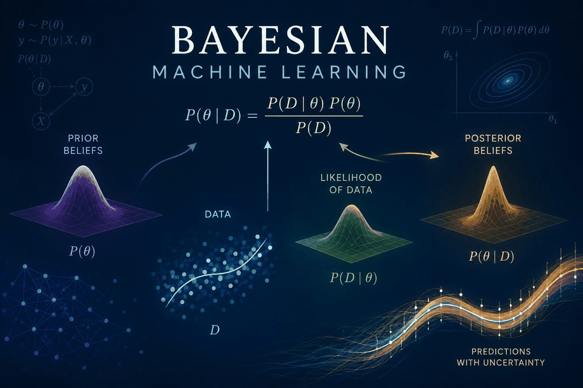
Given data x {\displaystyle x\,\!} and parameter θ {\displaystyle \theta } , a simple Bayesian analysis starts with a prior probability (prior) p ( θ ) {\displaystyle p(\theta )} and likelihood p ( x ∣ θ ) {\displaystyle p(x\mid \theta )} to compute a posterior probability p ( θ ∣ x ) ∝ p ( x ∣ θ ) p ( θ ) {\displaystyle p(\theta \mid x)\propto p(x\mid \theta )p(\theta )} . Often the prior on θ {\displaystyle \theta } depends in turn on other parameters φ {\displaystyle \varphi } that are not mentioned in the likelihood. So, the prior p ( θ ) {\displaystyle p(\theta )} must be replaced by a likelihood p ( θ ∣ φ ) {\displaystyle p(\theta \mid \varphi )} , and a prior p ( φ ) {\displaystyle p(\varphi )} on the newly introduced parameters φ {\displaystyle \varphi } is required, resulting in a posterior probability
p ( θ , φ ∣ x ) ∝ p ( x ∣ θ ) p ( θ ∣ φ ) p ( φ ) . {\displaystyle p(\theta ,\varphi \mid x)\propto p(x\mid \theta )p(\theta \mid \varphi )p(\varphi ).}
This is the simplest example of a hierarchical Bayes model. The process may be repeated; for example, the parameters φ {\displaystyle \varphi } may depend in turn on additional parameters ψ {\displaystyle \psi \,\!} , which require their own prior. Eventually the process must terminate, with priors that do not depend on unmentioned parameters.
Given the measured quantities x 1 , … , x n {\displaystyle x_{1},\dots ,x_{n}\,\!} each with normally distributed errors of known standard deviation σ {\displaystyle \sigma \,\!} ,
3. Dataset Ingestion, Preprocessing & Stochastic Augmentations
x i ∼ N ( θ i , σ 2 ) {\displaystyle x_{i}\sim N(\theta _{i},\sigma ^{2})}
Suppose we are interested in estimating the θ i {\displaystyle \theta _{i}} . An approach would be to estimate the θ i {\displaystyle \theta _{i}} using a maximum likelihood approach; since the observations are independent, the likelihood factorizes and the maximum likelihood estimate is simply
θ i = x i . {\displaystyle \theta _{i}=x_{i}.}
However, if the quantities are related, so that for example the individual θ i {\displaystyle \theta _{i}} have themselves been drawn from an underlying distribution, then this relationship destroys the independence and suggests a more complex model, e.g.,
x i ∼ N ( θ i , σ 2 ) , {\displaystyle x_{i}\sim N(\theta _{i},\sigma ^{2}),}
θ i ∼ N ( φ , τ 2 ) , {\displaystyle \theta _{i}\sim N(\varphi ,\tau ^{2}),}
with improper priors φ ∼ flat {\displaystyle \varphi \sim {\text{flat}}} , τ ∼ flat ∈ ( 0 , ∞ ) {\displaystyle \tau \sim {\text{flat}}\in (0,\infty )} . When n ≥ 3 {\displaystyle n\geq 3} , this is an identified model (i.e. there exists a unique solution for the model's parameters), and the posterior distributions of the individual θ i {\displaystyle \theta _{i}} will tend to move, or shrink away from the maximum likelihood estimates towards their common mean. This shrinkage is a typical behavior in hierarchical Bayes models.
Several equivalent definitions of a Bayesian network have been offered. For the following, let G = (V,E) be a directed acyclic graph (DAG) and let X = (Xv), v ∈ V be a set of random variables indexed by V.
p ( x ) = ∏ v ∈ V p ( x v | x pa ( v ) ) {\displaystyle p(x)=\prod _{v\in V}p\left(x_{v}\,{\big |}\,x_{\operatorname {pa} (v)}\right)}
where pa(v) is the set of parents of v (i.e. those vertices pointing directly to v via a single edge). For any set of random variables, the probability of any member of a joint distribution can be calculated from conditional probabilities using the chain rule (given a topological ordering of X) as follows:
P ( X 1 = x 1 , … , X n = x n ) = ∏ v = 1 n P ( X v = x v ∣ X v + 1 = x v + 1 , … , X n = x n ) {\displaystyle \operatorname {P} (X_{1}=x_{1},\ldots ,X_{n}=x_{n})=\prod _{v=1}^{n}\operatorname {P} \left(X_{v}=x_{v}\mid X_{v+1}=x_{v+1},\ldots ,X_{n}=x_{n}\right)}
4. Neural Network Backbone, Layer Specifications & Loss Formulations
P ( X 1 = x 1 , … , X n = x n ) = ∏ v = 1 n P ( X v = x v ∣ X j = x j for each X j that is a parent of X v ) {\displaystyle \operatorname {P} (X_{1}=x_{1},\ldots ,X_{n}=x_{n})=\prod _{v=1}^{n}\operatorname {P} (X_{v}=x_{v}\mid X_{j}=x_{j}{\text{ for each }}X_{j}\,{\text{ that is a parent of }}X_{v}\,)}
The difference between the two expressions is the conditional independence of the variables from any of their non-descendants, given the values of their parent variables.
X v ⊥ ⊥ X V ∖ de ( v ) ∣ X pa ( v ) for all v ∈ V {\displaystyle X_{v}\perp \!\!\!\perp X_{V\,\smallsetminus \,\operatorname {de} (v)}\mid X_{\operatorname {pa} (v)}\quad {\text{for all }}v\in V}
where de(v) is the set of descendants and V \ de(v) is the set of non-descendants of v. This can be expressed in terms similar to the first definition, as
P ( X v = x v ∣ X i = x i for each X i that is not a descendant of X v ) =
P ( X v = x v ∣ X j = x j for each X j that is a parent of X v ) {\displaystyle {\begin{aligned}&\operatorname {P} (X_{v}=x_{v}\mid X_{i}=x_{i}{\text{ for each }}X_{i}{\text{ that is not a descendant of }}X_{v}\,)\\[6pt]={}&P(X_{v}=x_{v}\mid X_{j}=x_{j}{\text{ for each }}X_{j}{\text{ that is a parent of }}X_{v}\,)\end{aligned}}}
P contains (but does not need to be entirely) a directed chain, u ⋯ ← m ← ⋯ v {\displaystyle u\cdots \leftarrow m\leftarrow \cdots v} or u ⋯ → m → ⋯ v {\displaystyle u\cdots \rightarrow m\rightarrow \cdots v} , such that the middle node m is in Z, P contains a fork, u ⋯ ← m → ⋯ v {\displaystyle u\cdots \leftarrow m\rightarrow \cdots v} , such that the middle node m is in Z, or P contains an inverted fork (or collider), u ⋯ → m ← ⋯ v {\displaystyle u\cdots \rightarrow m\leftarrow \cdots v} , such that the middle node m is not in Z and no descendant of m is in Z. The nodes u and v are d-separated by Z if all trails between them are d-separated. If u and v are not d-separated, they are d-connected. X is a Bayesian network with respect to G if, for any two nodes u, v:
X u ⊥ ⊥ X v ∣ X Z {\displaystyle X_{u}\perp \!\!\!\perp X_{v}\mid X_{Z}}
where Z is a set which d-separates u and v. (The Markov blanket is the minimal set of nodes which d-separates node v from all other nodes.)
a → b → c and a ← b ← c {\displaystyle a\rightarrow b\rightarrow c\qquad {\text{and}}\qquad a\leftarrow b\leftarrow c}
are equivalent: that is they impose exactly the same conditional independence requirements. A causal network is a Bayesian network with the requirement that the relationships be causal. The additional semantics of causal networks specify that if a node X is actively caused to be in a given state x (an action written as do(X = x)), then the probability density function changes to that of the network obtained by cutting the links from the parents of X to X, and setting X to the caused value x. Using these semantics, the impact of external interventions from data obtained prior to intervention can be predicted.
5. Training Protocol, Convergence Behavior & Experimental Evaluation
OpenBUGS – Open-source development of WinBUGS. SPSS Modeler – Commercial software that includes an implementation for Bayesian networks. Stan (software) – Stan is an open-source package for obtaining Bayesian inference using the No-U-Turn sampler (NUTS), a variant of Hamiltonian Monte Carlo. WinBUGS – One of the first computational implementations of MCMC samplers. No longer maintained.
the often subjective nature of the input information the reliance on Bayes' conditioning as the basis for updating information the distinction between causal and evidential modes of reasoning In the late 1980s Pearl's Probabilistic Reasoning in Intelligent Systems and Neapolitan's Probabilistic Reasoning in Expert Systems summarized their properties and established them as a field of study.
Artificial intelligence (AI) is the capability of computational systems to perform tasks typically associated with human intelligence, such as learning, reasoning, problem-solving, perception, and decision-making. It is also a field of research spanning computer science, engineering, and mathematics that develops and studies methods and software enabling machines to perceive their environment and use learning and intelligence to take actions that maximise their chances of achieving defined goals. Prominent applications of AI include advanced web search engines, chatbots, virtual assistants, autonomous vehicles, play and analysis in strategy games (e.g., chess and Go), and content generation (e.g., text, images, audio, and videos). The traditional goals of AI research include learning, reasoning, knowledge representation, planning, natural language processing, and perception, as well as support for robotics. To reach these goals, AI researchers use techniques including state space search and mathematical optimisation, formal logic, artificial neural networks, and methods based on statistics, operations research, and economics. AI also draws upon psychology, linguistics, philosophy, neuroscience, and other fields. Some companies, such as OpenAI, Google DeepMind, and Meta, aim to create artificial general intelligence (AGI)—AI that can complete nearly any cognitive task at least as well as a human. Artificial intelligence was founded as an academic discipline in 1956. The field went through multiple cycles of optimism throughout its history, followed by periods of disappointment and loss of funding, known as AI winters. Funding and interest increased substantially after 2012, when graphics processing units (GPUs) started being used to accelerate neural networks, and deep learning outperformed previous AI techniques. This growth accelerated further after 2017 with the transformer architecture. The 2020s AI boom was spurred on largely by advances in generative AI, which can create and modify media. In addition to AI safety and unintended consequences and harms from the use of AI, ethical concerns, AI's long-term effects, environmental effects, and potential existential risks have prompted discussions of AI regulation.
AI programs use knowledge to answer questions intelligently and make deductions about real-world facts. Formal knowledge representation and knowledge engineering use symbols to represent words, concepts and things in the world. A knowledge base is a body of knowledge represented in a form that can be used by a program. An ontology is the set of objects, relations, concepts, and properties used by a particular domain of knowledge. Formal knowledge has been studied extensively since the 1970s and researchers have developed formalisms for a wide variety of difficult domains. The symbolic approach has difficulty with several problems: the breadth of commonsense knowledge (the set of atomic facts the average person knows is enormous), the sub-symbolic form of most commonsense knowledge (much of what people know is not represented as "facts" or "statements" they can express verbally), and knowledge acquisition (the problem of obtaining knowledge for AI applications). Large language models (and some other AI programs developed since 2012) do not require explicit, symbolic knowledge. They acquire knowledge by being trained on the combined text of millions of books and billions of websites. Modern AI can also learn about a domain by running experiments (as when AlphaZero learns game strategy by playing against itself). Machine learning solves the problems of general knowledge, commonsense knowledge and knowledge acquisition, however, this approach has struggled with accurate recall and valid reasoning.
Unsupervised learning analyses a stream of data, finds patterns, and makes predictions without any other guidance. Supervised learning requires labelling the training data with the expected answers, and comes in two main varieties: classification (where the program must learn to predict what category the input belongs in) and regression (where the program must deduce a numeric function based on numeric input). Reinforcement learning is when the agent is rewarded for good responses and punished for bad ones. The agent learns to choose responses that are classified as "good". Transfer learning is when the knowledge gained from one problem is applied to a new problem. Deep learning is a type of machine learning that runs inputs through biologically inspired artificial neural networks for all of these types of learning. Computational learning theory can assess learners by computational complexity, sample complexity (how much data is required), or other notions of optimisation.
Affective computing is a field that comprises systems that recognise, interpret, process, or simulate human affect (feeling, emotion, and mood). For example, some virtual assistants are programmed to speak conversationally or even banter humorously; it makes them appear more sensitive to the emotional dynamics of human interaction, or to otherwise facilitate human–computer interaction. However, this tends to give naïve users an unrealistic conception of the intelligence of existing computer agents. Moderate successes related to affective computing include textual sentiment analysis and, more recently, multimodal sentiment analysis, wherein AI classifies the effects displayed by a videotaped subject.
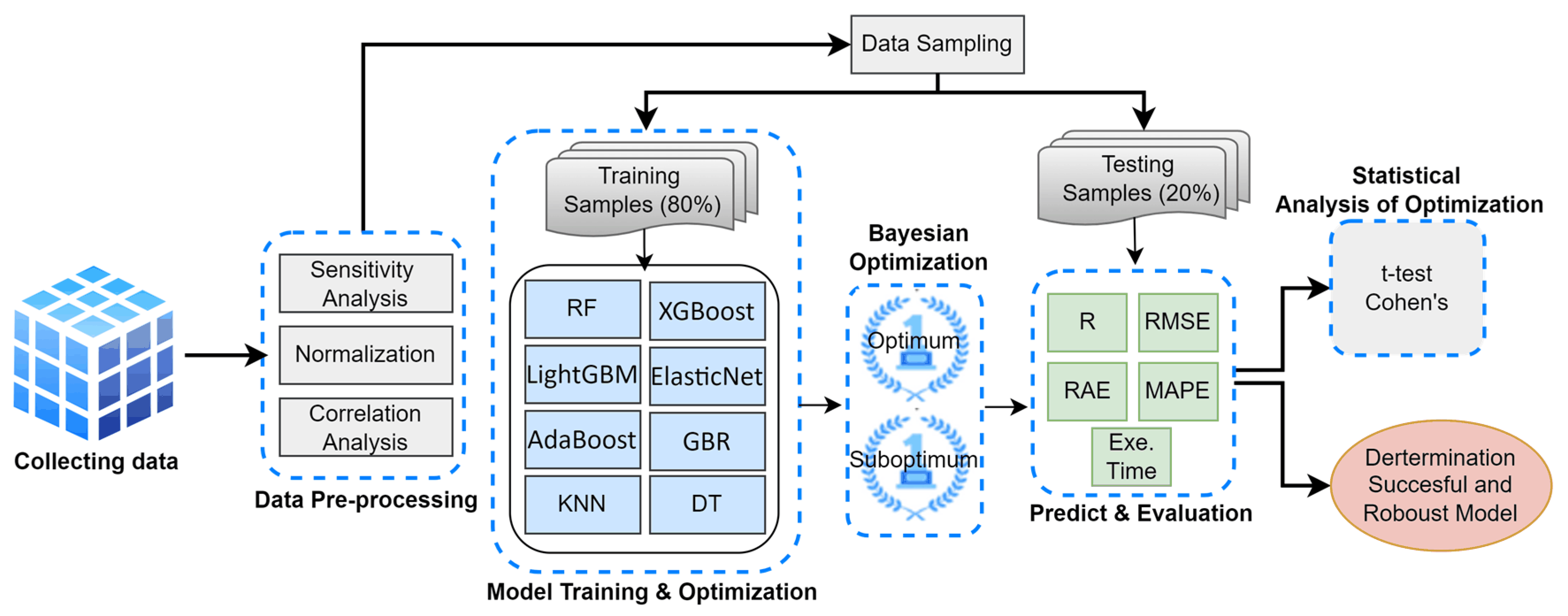
Local search uses mathematical optimisation to find a solution to a problem. It begins with some form of guess and refines it incrementally. Gradient descent is a type of local search that optimises a set of numerical parameters by incrementally adjusting them to minimise a loss function. Variants of gradient descent are commonly used to train neural networks, through the backpropagation algorithm. Another type of local search is evolutionary computation, which aims to iteratively improve a set of candidate solutions by "mutating" and "recombining" them, selecting only the fittest to survive each generation. Distributed search processes can coordinate via swarm intelligence algorithms. Two popular swarm algorithms used in search are particle swarm optimisation (inspired by bird flocking) and ant colony optimisation (inspired by ant trails).
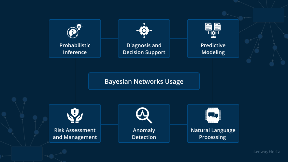
Many problems in AI (including reasoning, planning, learning, perception, and robotics) require the agent to operate with incomplete or uncertain information. AI researchers have devised a number of tools to solve these problems using methods from probability theory and economics. Precise mathematical tools have been developed that analyse how an agent can make choices and plan, using decision theory, decision analysis, and information value theory. These tools include models such as Markov decision processes, dynamic decision networks, game theory, and mechanism design. Bayesian networks are a tool that can be used for reasoning (using the Bayesian inference algorithm), learning (using the expectation–maximisation algorithm), planning (using decision networks) and perception (using dynamic Bayesian networks). Probabilistic algorithms can also be used for filtering, prediction, smoothing, and finding explanations for streams of data, thus helping perception systems analyse processes that occur over time (e.g., hidden Markov models or Kalman filters).
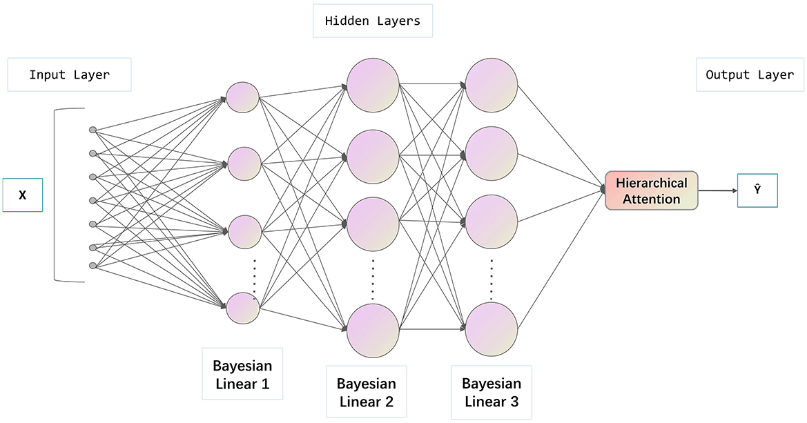
An artificial neural network is based on a collection of nodes also known as artificial neurons, which loosely model the neurons in a biological brain. It is trained to recognise patterns; once trained, it can recognise those patterns in fresh data. There is an input, at least one hidden layer of nodes and an output. Each node applies a function and once the weight crosses its specified threshold, the data is transmitted to the next layer. A network is typically called a deep neural network if it has at least 2 hidden layers. Learning algorithms for neural networks use local search to choose the weights that will get the right output for each input during training. The most common training technique is the backpropagation algorithm. Neural networks learn to model complex relationships between inputs and outputs and find patterns in data. In theory, a neural network can learn any function. In feedforward neural networks the signal passes in only one direction. The term perceptron typically refers to a single-layer neural network. In contrast, deep learning uses many layers. Recurrent neural networks (RNNs) feed the output signal back into the input, which allows short-term memories of previous input events. Long short-term memory networks (LSTMs) are recurrent neural networks that better preserve long-term dependencies and are less sensitive to the vanishing gradient problem. Convolutional neural networks (CNNs) use layers of kernels to more efficiently process local patterns. This local processing is especially important in image processing, where the early CNN layers typically identify simple local patterns such as edges and curves, with subsequent layers detecting more complex patterns like textures, and eventually whole objects.
Deep learning uses several layers of neurons between the network's inputs and outputs. The multiple layers can progressively extract higher-level features from the raw input. For example, in image processing, lower layers may identify edges, while higher layers may identify the concepts relevant to a human such as digits, letters, or faces. Deep learning improves the performance of computer vision, speech recognition, natural language processing, image classification and many other applications.
In the late 2010s, graphics processing units (GPUs) that were increasingly designed with AI-specific enhancements and used with specialised TensorFlow software had replaced previously used central processing units (CPUs) as the dominant means for large-scale (commercial and academic) machine learning models' training. Specialised programming languages such as Prolog were used in early AI research, but general-purpose programming languages like Python have become predominant. The transistor density in integrated circuits has been observed to roughly double every 18 months—a trend known as Moore's law, named after the Intel co-founder Gordon Moore, who first identified it. Improvements in GPUs have been even faster, a trend sometimes called Huang's law, named after Nvidia co-founder and CEO Jensen Huang.
Model Figures & Evaluation Curves (4 Images)
Deep Learning Execution Pipeline
(Preprocessing)
(Feature Extraction)
(Self-Attention)
(Loss Optimization)