Ai Carbon Footprint Estimation | AI Final Year Project Report

Complete Technical Paper Content — Ai Carbon Footprint Estimation

1. Executive Abstract, Problem Formulation & Background

These datasets are used in machine learning (ML) research and have been cited in peer-reviewed academic journals. Datasets are an integral part of the field of machine learning. Major advances in this field can result from advances in learning algorithms (such as deep learning), computer hardware, and, less intuitively, the availability of high-quality training datasets. High-quality labeled training datasets for supervised and semi-supervised machine-learning algorithms are usually difficult and expensive to produce because of the large amount of time needed to label the data. Although they do not need to be labeled, high-quality unlabeled datasets for unsupervised learning can also be difficult and costly to produce. Many organizations, including governments, publish and share their datasets, often using common metadata formats (such as Croissant). The datasets are classified, based on the licenses, into two groups: open data and non-open data. The datasets from various governmental-bodies are presented in List of open government data sites. The datasets are ported on open data portals. They are made available for searching, depositing and accessing through interfaces like Open API. The datasets are made available as various sorted types and subtypes.

The data portal is classified based on its type of license. The open source license based data portals are known as open data portals which are used by many government organizations and academic institutions.

The data portal sometimes lists a wide variety of subtypes of datasets pertaining to many machine learning applications.

The data portals which are suitable for a specific subtype of machine learning application are listed in the subsequent sections.

**RTP set** – 35,087 stationary-point geometries (reactant, transition state and product) drawn from 11,961 elementary reactions, each labeled with density-functional energies, atomic forces and full Hessian matrices at the ωB97X-D/6-31G(d) level. **IRC set** – 34,248 structures along 600 minimum-energy reaction paths, used to test extrapolation beyond trained stationary points. **NMS set** – 62,527 off-equilibrium geometries generated by normal-mode sampling to probe model robustness under thermal perturbations. The collection underpins the study Does Hessian Data Improve the Performance of Machine Learning Potentials? and was used to train and benchmark the machine-learning interatomic potentials reported therein. The dataset itself is distributed under a CC licence via Figshare.

OpenML: Web platform with Python, R, Java, and other APIs for downloading hundreds of machine learning datasets, evaluating algorithms on datasets, and benchmarking algorithm performance against dozens of other algorithms. PMLB: A large, curated repository of benchmark datasets for evaluating supervised machine learning algorithms. Provides classification and regression datasets in a standardized format that are accessible through a Python API. Metatext NLP: https://metatext.io/datasets web repository maintained by community, containing nearly 1000 benchmark datasets, and counting. Provides many tasks from classification to QA, and various languages from English, Portuguese to Arabic. Appen: Off The Shelf and Open Source Datasets hosted and maintained by the company. These biological, image, physical, question answering, signal, sound, text, and video resources number over 250 and can be applied to over 25 different use cases.

A convolutional neural network (CNN) is a type of feedforward neural network that learns features via filter (or kernel) optimization. This type of deep learning network has been applied to process and make predictions from many different types of data including text, images and audio. CNNs are the de-facto standard in deep learning-based approaches to computer vision and image processing, and have only recently been replaced—in some cases—by newer architectures such as the transformer. Vanishing gradients and exploding gradients, seen during backpropagation in earlier neural networks, are prevented by the regularization that comes from using shared weights over fewer connections. For example, for each neuron in the fully-connected layer, 10,000 weights would be required for processing an image sized 100 × 100 pixels. However, applying cascaded convolution (or cross-correlation) kernels, only 25 weights for each convolutional layer are required to process 5x5-sized tiles. Higher-layer features are extracted from wider context windows, compared to lower-layer features. Some applications of CNNs include:

image and video recognition, recommender systems, image classification, image segmentation, medical image analysis, natural language processing, brain–computer interfaces, and financial time series. CNNs are also known as shift invariant or space invariant artificial neural networks, based on the shared-weight architecture of the convolution kernels or filters that slide along input features and provide translation-equivariant responses known as feature maps. Counter-intuitively, most convolutional neural networks are not invariant to translation, due to the downsampling operation they apply to the input. Feedforward neural networks are usually fully connected networks, that is, each neuron in one layer is connected to all neurons in the next layer. The "full connectivity" of these networks makes them prone to overfitting data. Typical ways of regularization, or preventing overfitting, include: penalizing parameters during training (such as weight decay) or trimming connectivity (skipped connections, dropout, etc.) Robust datasets also increase the probability that CNNs will learn the generalized principles that characterize a given dataset rather than the biases of a poorly-populated set. Convolutional networks were inspired by biological processes in that the connectivity pattern between neurons resembles the organization of the animal visual cortex. Individual cortical neurons respond to stimuli only in a restricted region of the visual field known as the receptive field. The receptive fields of different neurons partially overlap such that they cover the entire visual field. CNNs use relatively little pre-processing compared to other image classification algorithms. This means that the network learns to optimize the filters (or kernels) through automated learning, whereas in traditional algorithms these filters are hand-engineered. This simplifies and automates the process, enhancing efficiency and scalability overcoming human-intervention bottlenecks.

A convolutional neural network consists of an input layer, hidden layers and an output layer. In a convolutional neural network, the hidden layers include one or more layers that perform convolutions. Typically this includes a layer that performs a dot product of the convolution kernel with the layer's input matrix. This product is usually the Frobenius inner product, and its activation function is commonly ReLU. As the convolution kernel slides along the input matrix for the layer, the convolution operation generates a feature map, which in turn contributes to the input of the next layer. This is followed by other layers such as pooling layers, fully connected layers, and normalization layers. Here it should be noted how close a convolutional neural network is to a matched filter.

2. Related Work, Literature Survey & Algorithmic Foundations

Although fully connected feedforward neural networks can be used to learn features and classify data, this architecture is generally impractical for larger inputs (e.g., high-resolution images), which would require massive numbers of neurons because each pixel is a relevant input feature. A fully connected layer for an image of size 100 × 100 has 10,000 weights for each neuron in the second layer. Convolution reduces the number of free parameters, allowing the network to be deeper. For example, using a 5 × 5 tiling region, each with the same shared weights, requires only 25 neurons. Using shared weights means there are many fewer parameters, which helps avoid the vanishing gradients and exploding gradients problems seen during backpropagation in earlier neural networks. To speed processing, standard convolutional layers can be replaced by depthwise separable convolutional layers, which are based on a depthwise convolution followed by a pointwise convolution. The depthwise convolution is a spatial convolution applied independently over each channel of the input tensor, while the pointwise convolution is a standard convolution restricted to the use of 1 × 1 {\displaystyle 1\times 1} kernels.

A deconvolutional neural network is essentially the reverse of a CNN. It consists of deconvolutional layers and unpooling layers. A deconvolutional layer is the transpose of a convolutional layer. Specifically, a convolutional layer can be written as a multiplication with a matrix, and a deconvolutional layer is multiplication with the transpose of that matrix. An unpooling layer expands the layer. The max-unpooling layer is the simplest, as it simply copies each entry multiple times. For example, a 2-by-2 max-unpooling layer is [ x ] ↦ [ x x x x ] {\displaystyle [x]\mapsto {\begin{bmatrix}x&x\\x&x\end{bmatrix}}} . Deconvolution layers are used in image generators. By default, it creates periodic checkerboard artifact, which can be fixed by upscale-then-convolve.

Work by Hubel and Wiesel in the 1950s and 1960s showed that cat visual cortices contain neurons that individually respond to small regions of the visual field. Provided the eyes are not moving, the region of visual space within which visual stimuli affect the firing of a single neuron is known as its receptive field. Neighboring cells have similar and overlapping receptive fields. Receptive field size and location varies systematically across the cortex to form a complete map of visual space. The cortex in each hemisphere represents the contralateral visual field. Their 1968 paper identified two basic visual cell types in the brain:

simple cells, whose output is maximized by straight edges having particular orientations within their receptive field complex cells, which have larger receptive fields, whose output is insensitive to the exact position of the edges in the field. Hubel and Wiesel also proposed a cascading model of these two types of cells for use in pattern recognition tasks.

"S-layer": a shared-weights receptive-field layer, later known as a convolutional layer, which contains units whose receptive fields cover a patch of the previous layer. A shared-weights receptive-field group (a "plane" in neocognitron terminology) is often called a filter, and a layer typically has several such filters. "C-layer": a downsampling layer that contain units whose receptive fields cover patches of previous convolutional layers. Such a unit typically computes a weighted average of the activations of the units in its patch, and applies inhibition (divisive normalization) pooled from a somewhat larger patch and across different filters in a layer, and applies a saturating activation function. The patch weights are nonnegative and are not trainable in the original neocognitron. The downsampling and competitive inhibition help to classify features and objects in visual scenes even when the objects are shifted. Several supervised and unsupervised learning algorithms have been proposed over the decades to train the weights of a neocognitron. Today, however, the CNN architecture is usually trained through backpropagation. Fukushima's ReLU activation function was not used in his neocognitron since all the weights were nonnegative; lateral inhibition was used instead. The rectifier has become a very popular activation function for CNNs and deep neural networks in general.

LeNet-5, a pioneering 7-level convolutional network by LeCun et al. in 1995, classifies hand-written numbers on checks digitized in 32×32 pixel images. The ability to process higher-resolution images requires larger and more layers of convolutional neural networks, so this technique is constrained by the availability of computing resources. It was superior than other commercial courtesy amount reading systems (as of 1995). The system was integrated in NCR's check reading systems, and fielded in several American banks since June 1996, reading millions of checks per day.

For example, in CIFAR-10, images are only of size 32×32×3 (32 wide, 32 high, 3 color channels), so a single fully connected neuron in the first hidden layer of a regular neural network would have 32*32*3 = 3,072 weights. A 200×200 image, however, would lead to neurons that have 200*200*3 = 120,000 weights. Also, such network architecture does not take into account the spatial structure of data, treating input pixels which are far apart in the same way as pixels that are close together. This ignores locality of reference in data with a grid-topology (such as images), both computationally and semantically. Thus, full connectivity of neurons is wasteful for purposes such as image recognition that are dominated by spatially local input patterns. Convolutional neural networks are variants of multilayer perceptrons, designed to emulate the behavior of a visual cortex. These models mitigate the challenges posed by the MLP architecture by exploiting the strong spatially local correlation present in natural images. As opposed to MLPs, CNNs have the following distinguishing features:

3D volumes of neurons. The layers of a CNN have neurons arranged in 3 dimensions: width, height and depth. Each neuron inside a convolutional layer is connected to only a small region of the layer before it, called a receptive field. Distinct types of layers, both locally and completely connected, are stacked to form a CNN architecture. Local connectivity: following the concept of receptive fields, CNNs exploit spatial locality by enforcing a local connectivity pattern between neurons of adjacent layers. The architecture thus ensures that the learned "filters" produce the strongest response to a spatially local input pattern. Stacking many such layers leads to nonlinear filters that become increasingly global (i.e. responsive to a larger region of pixel space) so that the network first creates representations of small parts of the input, then from them assembles representations of larger areas. Shared weights: In CNNs, each filter is replicated across the entire visual field. These replicated units share the same parameterization (weight vector and bias) and form a feature map. This means that all the neurons in a given convolutional layer respond to the same feature within their specific response field. Replicating units in this way allows for the resulting activation map to be equivariant under shifts of the locations of input features in the visual field, i.e. they grant translational equivariance—given that the layer has a stride of one. Pooling: In a CNN's pooling layers, feature maps are divided into rectangular sub-regions, and the features in each rectangle are independently down-sampled to a single value, commonly by taking their average or maximum value. In addition to reducing the sizes of feature maps, the pooling operation grants a degree of local translational invariance to the features contained therein, allowing the CNN to be more robust to variations in their positions. Together, these properties allow CNNs to achieve better generalization on vision problems. Weight sharing dramatically reduces the number of free parameters learned, thus lowering the memory requirements for running the network and allowing the training of larger, more powerful networks.

The convolutional layer is the core building block of a CNN. The layer's parameters consist of a set of learnable filters (or kernels), which have a small receptive field, but extend through the full depth of the input volume. During the forward pass, each filter is convolved across the width and height of the input volume, computing the dot product between the filter entries and the input, producing a 2-dimensional activation map of that filter. As a result, the network learns filters that activate when it detects some specific type of feature at some spatial position in the input. Stacking the activation maps for all filters along the depth dimension forms the full output volume of the convolution layer. Every entry in the output volume can thus also be interpreted as an output of a neuron that looks at a small region in the input. Each entry in an activation map use the same set of parameters that define the filter. Self-supervised learning has been adapted for use in convolutional layers by using sparse patches with a high-mask ratio and a global response normalization layer.

3. Dataset Ingestion, Preprocessing & Stochastic Augmentations

When dealing with high-dimensional inputs such as images, it is impractical to connect neurons to all neurons in the previous volume because such a network architecture does not take the spatial structure of the data into account. Convolutional networks exploit spatially local correlation by enforcing a sparse local connectivity pattern between neurons of adjacent layers: each neuron is connected to only a small region of the input volume. The extent of this connectivity is a hyperparameter called the receptive field of the neuron. The connections are local in space (along width and height), but always extend along the entire depth of the input volume. Such an architecture ensures that the learned filters produce the strongest response to a spatially local input pattern.

The depth of the output volume controls the number of neurons in a layer that connect to the same region of the input volume. These neurons learn to activate for different features in the input. For example, if the first convolutional layer takes the raw image as input, then different neurons along the depth dimension may activate in the presence of various oriented edges, or blobs of color. Stride controls how depth columns around the width and height are allocated. If the stride is 1, then we move the filters one pixel at a time. This leads to heavily overlapping receptive fields between the columns, and to large output volumes. For any integer S > 0 , {\textstyle S>0,} a stride S means that the filter is translated S units at a time per output. In practice, S ≥ 3 {\textstyle S\geq 3} is rare. A greater stride means smaller overlap of receptive fields and smaller spatial dimensions of the output volume. Sometimes, it is convenient to pad the input with zeros (or other values, such as the average of the region) on the border of the input volume. The size of this padding is a third hyperparameter. Padding provides control of the output volume's spatial size. In particular, sometimes it is desirable to exactly preserve the spatial size of the input volume, this is commonly referred to as "same" padding.

The spatial size of the output volume is a function of the input volume size W {\displaystyle W} , the kernel field size K {\displaystyle K} of the convolutional layer neurons, the stride S {\displaystyle S} , and the amount of zero padding P {\displaystyle P} on the border. The number of neurons that "fit" in a given volume is then:

W − K + 2 P S + 1. {\displaystyle {\frac {W-K+2P}{S}}+1.}

If this number is not an integer, then the strides are incorrect and the neurons cannot be tiled to fit across the input volume in a symmetric way. In general, setting zero padding to be P = ( K − 1 ) / 2 {\textstyle P=(K-1)/2} when the stride is S = 1 {\displaystyle S=1} ensures that the input volume and output volume will have the same size spatially. However, it is not always completely necessary to use all of the neurons of the previous layer. For example, a neural network designer may decide to use just a portion of padding.

Another important concept of CNNs is pooling, which is used as a form of non-linear down-sampling. Pooling provides downsampling because it reduces the spatial dimensions (height and width) of the input feature maps while retaining the most important information. There are several non-linear functions to implement pooling, where max pooling and average pooling are the most common. Pooling aggregates information from small regions of the input creating partitions of the input feature map, typically using a fixed-size window (like 2x2) and applying a stride (often 2) to move the window across the input. Note that without using a stride greater than 1, pooling would not perform downsampling, as it would simply move the pooling window across the input one step at a time, without reducing the size of the feature map. In other words, the stride is what actually causes the downsampling by determining how much the pooling window moves over the input. Intuitively, the exact location of a feature is less important than its rough location relative to other features. This is the idea behind the use of pooling in convolutional neural networks. The pooling layer serves to progressively reduce the spatial size of the representation, to reduce the number of parameters, memory footprint and amount of computation in the network, and hence to also control overfitting. This is known as down-sampling. It is common to periodically insert a pooling layer between successive convolutional layers (each one typically followed by an activation function, such as a ReLU layer) in a CNN architecture. While pooling layers contribute to local translation invariance, they do not provide global translation invariance in a CNN, unless a form of global pooling is used. The pooling layer commonly operates independently on every depth, or slice, of the input and resizes it spatially. A very common form of max pooling is a layer with filters of size 2×2, applied with a stride of 2, which subsamples every depth slice in the input by 2 along both width and height, discarding 75% of the activations: f X , Y ( S ) = max a , b = 0 1 S 2 X + a , 2 Y + b . {\displaystyle f_{X,Y}(S)=\max _{a,b=0}^{1}S_{2X+a,2Y+b}.}

In this case, every max operation is over 4 numbers. The depth dimension remains unchanged (this is true for other forms of pooling as well). In addition to max pooling, pooling units can use other functions, such as average pooling or ℓ2-norm pooling. Average pooling was often used historically but has recently fallen out of favor compared to max pooling, which generally performs better in practice. Due to the effects of fast spatial reduction of the size of the representation, there is a recent trend towards using smaller filters or discarding pooling layers altogether.

The "loss layer", or "loss function", exemplifies how training penalizes the deviation between the predicted output of the network, and the true data labels (during supervised learning). Various loss functions can be used, depending on the specific task. The Softmax loss function is used for predicting a single class of K mutually exclusive classes. Sigmoid cross-entropy loss is used for predicting K independent probability values in [ 0 , 1 ] {\displaystyle [0,1]} . Euclidean loss is used for regressing to real-valued labels ( − ∞ , ∞ ) {\displaystyle (-\infty ,\infty )} .

Hyperparameters are various settings that are used to control the learning process. CNNs use more hyperparameters than a standard multilayer perceptron (MLP).

4. Neural Network Backbone, Layer Specifications & Loss Formulations

Regularization is a process of introducing additional information to solve an ill-posed problem or to prevent overfitting. CNNs use various types of regularization.

Because the degree of model overfitting is determined by both its power and the amount of training it receives, providing a convolutional network with more training examples can reduce overfitting. Because there is often not enough available data to train, especially considering that some part should be spared for later testing, two approaches are to either generate new data from scratch (if possible) or perturb existing data to create new ones. The latter one is used since mid-1990s. For example, input images can be cropped, rotated, or rescaled to create new examples with the same labels as the original training set.

One of the simplest methods to prevent overfitting of a network is to simply stop the training before overfitting has had a chance to occur. It comes with the disadvantage that the learning process is halted.

Convolutional deep belief networks (CDBN) have structure very similar to convolutional neural networks and are trained similarly to deep belief networks. Therefore, they exploit the 2D structure of images, like CNNs do, and make use of pre-training like deep belief networks. They provide a generic structure that can be used in many image and signal processing tasks. Benchmark results on standard image datasets like CIFAR have been obtained using CDBNs.

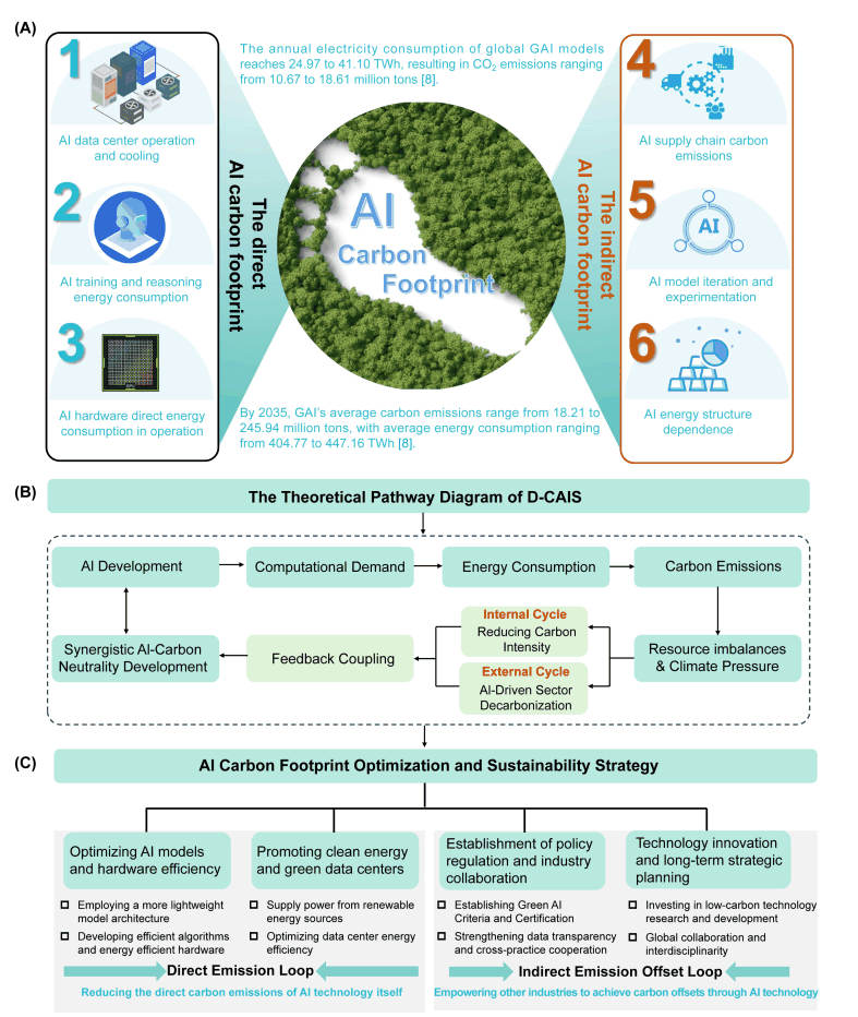
Establishing a carbon accounting system is the foundational step for implementing Green AI. This guide introduces the core methodologies and tools you need to start measuring the environmental impact of your AI workloads.

Measuring your AI's carbon footprint begins with selecting a robust calculation methodology. Frameworks like Green Algorithms or the Machine Learning Emissions Calculator provide the formulas to convert cloud compute usage into CO2 equivalent emissions. You must instrument your training and inference pipelines to capture key data: GPU/CPU hours , memory usage , and the carbon intensity of your cloud provider's energy grid. This data forms the basis for accurate Scope 2 emissions reporting, which covers purchased electricity.

To operationalize measurement, integrate monitoring libraries like CodeCarbon or Carbontracker directly into your code. These tools automatically log energy consumption data during model runs. The final step is building a centralized reporting dashboard, using tools like Grafana , to visualize emissions per project, team, or model. This dashboard turns raw data into actionable insights, enabling you to set reduction targets and prioritize optimizations, a practice aligned with our guide on How to Establish Green AI Governance and KPIs .

5. Training Protocol, Convergence Behavior & Experimental Evaluation

Establishing a robust measurement framework is the first step to reducing your AI's environmental impact. These core concepts provide the building blocks for a practical carbon accounting system.

Green Algorithms is an open-source framework for estimating the carbon footprint of computational research. It provides a standardized methodology to calculate emissions based on: CPU/GPU runtime and hardware type Power Usage Effectiveness (PUE) of the data center Carbon intensity of the local electricity grid Use it to establish a baseline for your training and inference jobs, moving from vague concerns to quantifiable metrics. It's the de facto starting point for academic and industrial carbon accounting.

Green Algorithms is an open-source framework for estimating the carbon footprint of computational research. It provides a standardized methodology to calculate emissions based on:

Use it to establish a baseline for your training and inference jobs, moving from vague concerns to quantifiable metrics. It's the de facto starting point for academic and industrial carbon accounting.

For AI developers, Scope 2 emissions —indirect emissions from purchased electricity—are the primary carbon source. You must track: Energy consumption of your virtual machines and accelerators The grid carbon intensity of your cloud region (e.g., AWS us-west-2 vs. eu-central-1) Data center PUE , a multiplier for cooling and overhead Tools like AWS Customer Carbon Footprint Tool and Google Cloud Carbon Footprint provide this data. Allocating these emissions to specific projects is essential for actionable reporting.

For AI developers, Scope 2 emissions —indirect emissions from purchased electricity—are the primary carbon source. You must track:

Tools like AWS Customer Carbon Footprint Tool and Google Cloud Carbon Footprint provide this data. Allocating these emissions to specific projects is essential for actionable reporting.