Complete Technical Paper Content — Ai Chemistry Projects
1. Executive Abstract, Problem Formulation & Background
arXivLabs is a framework that allows collaborators to develop and share new arXiv features directly on our website.
2. Related Work, Literature Survey & Algorithmic Foundations
Both individuals and organizations that work with arXivLabs have embraced and accepted our values of openness, community, excellence, and user data privacy. arXiv is committed to these values and only works with partners that adhere to them.
3. Dataset Ingestion, Preprocessing & Stochastic Augmentations
Have an idea for a project that will add value for arXiv's community? Learn more about arXivLabs .
4. Neural Network Backbone, Layer Specifications & Loss Formulations
AutoMix: Automatically Mixing Language Models Pranjal Aggarwal Thanks: *Equal Contribution. Work started and partly done during Aman’s internship at Google. Aman Madaan 1 1 footnotemark: 1 Ankit Anand Srividya Pranavi Potharaju Swaroop Mishra Pei ZhouAditya Gupta Dheeraj Rajagopal Karthik Kappaganthu Yiming Yang Shyam Upadhyay Manaal Faruqui Mausam ♠ \spadesuit Carnegie Mellon University ♣ \clubsuit xAI † \dagger Google ‡ \ddagger Google DeepMind ♢ \diamondsuit IIT Delhi △ \bigtriangleup University of Southern California automix-models@googlegroups.com Abstract Large language models (LLMs) are now available from cloud API providers in various sizes and configurations. While this diversity offers a broad spectrum of choices, effectively leveraging the options to optimize computational cost and performance remains challenging. In this work, we present AutoMix , an approach that strategically routes queries to larger LMs, based on the approximate correctness of outputs from a smaller LM. Central to AutoMix are two key technical contributions. First, it has a few-shot self-verification mechanism, which estimates the reliability of its own outputs without requiring extensive training. Second, given that self-verification can be noisy, it employs a POMDP based router that can effectively select an appropriately sized model, based on answer confidence. Experiments across five language models and five challenging datasets show that AutoMix consistently surpasses strong baselines, reducing computational cost by over 50% for comparable performance. 1 1 1 Code available at github.com/automix-llm/automix 1 Introduction The landscape of Large Language Models (LLMs) is rapidly evolving, with a wide array of models now available in various sizes, capabilities, and computational requirements Touvron et al. 2023 ; OpenAI 2023 ; Jiang et al. 2023a . While larger models generally exhibit superior performance, their substantial computational costs render them unaffordable for many simpler tasks. Moreover, the vast array of available options makes it challenging for end-users to determine the optimal model configuration for their specific needs. This challenge is further compounded by the intrinsic complexity and variability of real-world tasks, ranging from simple (e.g., binary classification on separable data) to complex (e.g., code generation) and potentially unsolvable tasks (e.g., certain forms of multi-step reasoning). To address these issues and ensure that end-users can obtain the best performance within their budget constraints, the development of model-switching techniques has become increasingly important. These techniques involve dispatching queries to models of disparate sizes and capabilities, allowing for a more efficient allocation of computational resources ( Liu et al. 2020 ; Zhou et al. 2020 ; Madaan and Yang 2022 ; Geng et al. 2021 ; Schuster et al. 2022 ) . Figure 1 : Representative example for 2 model setup in AutoMix . Instead of relying only on small model ( SLM ) with low performance or a large model ( LLM ) with high cost, AutoMix automatically mixes multiple black-box language models, based on user desired cost-quality tradeoff. AutoMix works in a 3-step process: 1.) generation by a small model ( L M 1 LM_{1} ), 2.) self-verification of the generated answer, 3.) using confidence assessments from self-verification to do appropriate routing to a larger model ( L M 2 LM_{2} ). For N-model setup, the process is repeated till the final answer is reported. Contemporary model-switching strategies often rely on separate routing models trained for a fixed set of tasks ( Chen et al. 2023 ; Ding et al. 2024 ) . Moreover, modern LLMs are frequently accessible only through black-box APIs, restricting direct model optimization due to the unavailability of fine-tuning capabilities and weight access. This constraint, coupled with the expectation of access to large amounts of task-specific data, creates a challenge that existing routing approaches fail to address adequately. In response, we introduce AutoMix , a method that enables users to mix models of various sizes and capabilities, assuming only access to black-box LLM APIs. As illustrated in Figure 1 , AutoMix consists of 3 steps designed within the constraints of black-box access: solution generation (small model to generate initial answer), self-verification (same smaller model assesses difficulty), and selective routing (routing to larger models when suggested by self-verification). At a high level, this process mirrors human problem-solving, which inherently follows a multi-step process: generate a solution, verify its validity, and refine it further based on verification outcomes. An ideal router in AutoMix must incorporate several key characteristics. Firstly, it should be capable of identifying the difficulty of a query based on confidence assessments of the smaller model’s answers. Secondly, it should be able to route to the appropriately sized model, for instance, easy queries are routed to the small language model ( SLM ), hard queries to large language model ( LLM ), and unlike previous works ( Chen et al. 2023 ; Ramírez et al. 2024 ) , unsolvable queries that no model can solve should not be routed to any LM, thereby saving costs. Thirdly, it should be able to learn from a small amount of data, as expected in real-world tasks. While self-verification seems a natural choice to provide confidence assessments and learn from limited data, prior works have shown self-verification is not particularly effective for reasoning tasks and is often noisy and ill-calibrated ( Tyen et al. 2023 ; Huang et al. 2023b ) – a challenge that needs to be addressed. Finally, the router should generalize to different scenarios in terms of the number of models with varying costs and capabilities. To address these requirements, we propose two novel contributions in AutoMix . First, we formulate self-verification as an entailment problem, where the consistency of the generated answer with the context is evaluated to estimate confidence levels Poliak 2020 ; Dagan et al. 2022 . For example, an answer discussing "apples" in a context focused on "tea" would be flagged as highly inconsistent. Second, we introduce a Partially Observable MDP (POMDP) based router Åström 1965 . POMDPs extend standard MDPs to decision problems where observations (self-verification probabilities) are unreliable and provide a noisy estimate of states (question difficulty). Modeling the router as a POMDP agent ensures all our requirements are met, as the POMDP can implicitly model various difficulties and assess them based on noisy self-verification outputs. Furthermore, POMDPs provide a principled formulation to learn robust routing policies in different scenarios with varying numbers of models, different costs, and capabilities, while learning from as few as 50 examples. We conduct extensive evaluations of AutoMix on five different dialogue and context-grounded reasoning tasks, with five different models. Our results demonstrate that AutoMix consistently outperforms baselines while reducing cost by over two times while achieving the same performance, showcasing significant improvements and efficiency gains over existing model-switching strategies. 2 Background and Related Work Self-Verification The concept of self-verification in reasoning problems has been explored in various works, such as Weng et al. 2023 ; Jiang et al. 2023b ; Pan et al. 2023a . These approaches typically rely on the LLM’s knowledge ( Dhuliawala et al. 2023 ) , a method that can pose challenges for reasoning problems ( Madaan et al. 2023 ; Huang et al. 2023b ) . In contrast, AutoMix leverages context for verification and introduces a POMDP router to mitigate potential noise from the verifier. Another line of work collects a corpus of past mistakes made by models Madaan et al. 2022 , and external knowledge bases for verification ( Peng et al. 2023 ; Gao et al. 2023 ; Pan et al. 2023b ) . In contrast, AutoMix uses the question’s context to verify the answer. While previous works find self-verification is unreliable to repair the model’s output Huang et al. 2023a , we demonstrate that self-verification provides a valuable signal used for routing to an appropriate model. Mixing Models Several works have sought to optimize LLM inference cost through model switching, employing specifically trained verifiers Chen et al. 2023 ; Zhu et al. 2023 ; vSakota et al. 2023 ; Ding et al. 2024 . AutoMix eliminates the need for expensive verifier training through few-shot SLM model prompting and does not require upfront access to all input queries. The router, trained with as few as 50 samples, outperforms specialized models. Our work is thus aligned with recent work that aims at composing different models and external tools for inference time improvement of language models ( Khattab et al. 2023 ; Press et al. 2022 ; Yao et al. 2022 ; Zhou et al. 2022 ) . Adaptive Computation Adaptive computation and model routing methods often preempt computation via intermediate representations ( Liu et al. 2020 ; Zhou et al. 2020 ; Geng et al. 2021 ; Schuster et al. 2022 ; Madaan and Yang 2022 ) . Unlike these methods, AutoMix requires no architectural changes and assumes only black-box access to APIs. While some black-box methods like AdaptiveConsistency ( Aggarwal et al. 2023 ) aim to optimize inference for reasoning tasks, they are limited to a single LLM model, whereas AutoMix flexibly optimizes between two or more models. Background on Partially Observable Markov Decision Processes POMDPs extend Markov Decision Processes (MDPs) to scenarios where an agent’s state observation is partial or noisy. Defined as a tuple ⟨ S , A , T , R , Ω , O ⟩ \langle S,A,T,R,\Omega,O\rangle , S S denotes states, A A actions, and Ω \Omega possible observations. The transition function T T gives transition probabilities between states given an action, while the observation function P P connects actions and states to observations. The reward function R R assigns rewards to actions in specific states. Agents in POMDPs maintain a belief ( b b ), a probability distribution over states. This belief updates based on actions and observations. The objective in a POMDP is to find a policy π : b ↦ a ∈ A \pi:b\mapsto a\in A that maximizes the expected cumulative long-term reward. POMDPs have been used in various domains, including robotics, automated navigation, crowdsourcing workflows, and strategic planning Kaelbling et al. 1998 ; Schwarting et al. 2018 ; Dai et al. 2010 ; Meuleau et al. 2013 . However, AutoMix uses POMDPs in a novel way to route queries between LMs. Our noisy self-verification outputs act as observations to the POMDP, which assesses question difficulty and routes to the appropriate LM to maximize a reward function of cost and performance. 3 Problem Formulation ⬇ Context : { context } Question : { question } AI Generated Answer : { generated_answer } Instruction : Your task is to evaluate if the AI Generated Answer is correct , based on the provided context and question . Provide the judgement and reasoning for each case . Choose between Correct or Incorrect . Evaluation :" List of codeblocks 1 Verification Prompt. The verification process is framed as a natural language entailment task, where the model determines the validity of the model-generated answer with respect to the context and question. We use a generic few-shot prompt for all tasks. We address the problem of selecting the appropriate language model (LM) to maximize a user-defined cost-quality tradeoff. We assume access to N N distinct language models: L M 1 , L M 2 … L M N LM_{1},LM_{2}\ldots LM_{N} , numbered in increasing order of number of parameters. Each model has an associated cost of C i C_{i} and (unknown) performance of P i P_{i} for each input query. Our objective is to maximize the total performance for any total cost while dynamically invoking any L M LM as appropriate for a given test point. In experiments, we compare cost-quality curves of various methods and also evaluate them using a newly proposed ibc metric (See Section 5.1 ). To test our approach, we consider context-grounded reasoning tasks, such as comprehension-based QA and a variety of dialogue reasoning tasks, where given a context 𝒞 \mathcal{C} (e.g., stories, newswire, or dialogue history) and a question q q , the model must generate an accurate and coherent answer consistent with the provided context. Our choice of tasks is motivated by two key considerations: (1) longer queries are more computationally demanding, underscoring the need for an approach like AutoMix to navigate the cost-accuracy tradeoff, and (2) the context allows for cross-checking preliminary answers with available information using self-verification (described shortly). We assume only black-box access is available to the LM APIs. For training any router models, we assume access to a small training/validation dataset 𝒟 t r a i n \mathcal{D}_{train} consisting of < 𝒞 , q , y ^ , y L M i > <\mathcal{C},q,\hat{y},y_{LM_{i}}> triplets, where y ^ \hat{y} is the ground truth answer and y L M i y_{LM_{i}} is the answer generated by L M i LM_{i} . 4 AutoMix At a high level, AutoMix consists of three steps: solution generation – using a small LM, say L M i LM_{i} (initially i = 1 i=1 ), to generate an answer 𝒜 s \mathcal{A}_{s} ; self-verification – using the same L M i LM_{i} to assess 𝒜 s \mathcal{A}_{s} ; and selective routing – picking a larger LM, L M j ( j > i CLOSE LM_{j}(j>i ), when suggested by self-verification, else returning 𝒜 s \mathcal{A}_{s} as final answer. Figure 1 shows a representative example of the process for the two-LM case. Next, we discuss our two technical contributions in detail. Figure 2: Context-Grounded Self-Verification using llama2-13b in Action. The example showcases the verifier, utilizing the same model as the answer generator, identifying and rejecting an inaccurate answer— He took it in 1990 —by effectively leveraging the context. 4.1 Self-Verification To assess the trustworthiness of 𝒜 s \mathcal{A}_{s} , AutoMix employs a few-shot verifier, 𝒱 \mathcal{V} , which validates L M i LM_{i} ’s output. Unlike existing works that perform verification by creating a new question ( Weng et al. 2022 ; Jiang et al. 2023b ) , we frame verification as an entailment task ( Dagan et al. 2005 ; Poliak 2020 ; Dagan et al. 2022 ) , to determine whether the answer generated by L M i LM_{i} aligns with the provided context. Specifically, the verifier gauges v = p ( correct = 1 ∣ 𝒜 s , 𝒞 , q ) v=\text{p}(\text{correct = 1}\mid\mathcal{A}_{s},\mathcal{C},q) , with correct = 1 =1 indicating that 𝒜 s \mathcal{A}_{s} is correct. To estimate the probability, we sample k > 1 k>1 times from the verifier ( L M i LM_{i} ) with high sampling temperature, and probability is then computed as 1 k ∑ i = 1 k 𝟏 { correct = 1 } \frac{1}{k}\sum_{i=1}^{k}\mathbf{1}\{\text{correct = 1}\} . We use the same 4-shot verification prompt for all tasks and do not train a verifier. Figure 1 , 2 shows the prompt and an example of self-verification in action. We refer readers to Appendix B for all prompts used. 4.2 Router Routing follows solution generation and self-verification. The router decides whether the output from L M i LM_{i} should be accepted or the query be routed to some L M j LM_{j} ( j > i j>i ) for improved performance. The router can also be interpreted as a meta-verifier , providing an extra layer of confidence assessment on the few-shot verifier’s evaluations. Specifically, 𝒱 \mathcal{V} ascertains whether L M i LM_{i} ’s answer is entailed by the context, making its decision without considering the inherent difficulty of the problem. For example, when handling Unsolvable queries, invoking a larger LM will be resource-inefficient and would not enhance performance. A good router can address this by not routing such a query further, and this decision needs to be made using the verification probability and trends from the training data. Addressing the notable challenges of self-correction in large language models ( Madaan et al. 2023 ; Huang et al. 2023b ) , AutoMix employs a non-LLM setup for routing and avoids escalating issues such as hallucination and reasoning errors ( Dziri et al. 2023 ) . The router can, in principle, adopt various learning strategies, including supervised learning, reinforcement learning, and symbolic reasoning. Subsequent sections provide details of two different routing strategies in AutoMix . Thresholding In this simplistic routing approach for the two-model case ( N = 2 N=2 ), the decision to route to L M 2 LM_{2} is based on the probability v v of the L M 1 LM_{1} verifier and a threshold t t . If v ≥ t v\geq t , it returns L M 1 LM_{1} ’s answer, else routes the query to L M 2 LM_{2} . Intuitively, a high probability indicates the verifier is confident in its decision and can be trusted. Varying t t can help explore cost-performance tradeoffs. POMDP-based Router A router should direct a query to larger LMs only when the performance gap justifies the cost-quality tradeoff. Given the inherent uncertainty in the true state of system performance, which remains unobserved, we formulate the router as a Partially Observable Markov Decision Process (POMDP) Åström 1965 . POMDPs are particularly well-suited for scenarios where observations, such as self-verification probabilities, may not be entirely reliable. Recall that ( Section 2 ) a POMDP is characterized by ( S , A , T , R , Ω , O ) (S,A,T,R,\Omega,O) . In our application, the states S S represent the current selected L M i LM_{i} and performance metrics (e.g., accuracy or F-score) of various LMs on a data point, denoted as S = ⟨ i , P e r f L M 1 , P e r f L M 2 , … , P e r f L M N ⟩ S=\langle{}i,Perf_{LM_{1}},Perf_{LM_{2}},\ldots,Perf_{LM_{N}}\rangle{} . The actions include either retaining the current LM’s ( L M i LM_{i} ) answer or routing to one of the larger LMs. Observations Ω \Omega , in the form of the verifier, outputs v v from L M i LM_{i} , enabling the POMDP to ascertain its belief state b b : a probability distribution over S S . The observation probabilities P ( o | s ) P(o|s) , which indicate the likelihood of observing o o (verification output) given state s s , are crucial for defining the POMDP model. E.g., high verifier confidence might suggest that the current LM’s performance P e r f L M i Perf_{LM_{i}} is high enough, reducing the necessity to switch to a more costly LM. The observation probabilities are estimated directly on the train set, by computing the expectation of verification probabilities for each state, i.e P ( o | s ) = ∑ s j , v j ∈ D t r a i n 𝟏 { s j = s and v j = o } ∑ s j ∈ D t r a i n 𝟏 { s j = s } P(o|s)=\frac{\sum_{s_{j},v_{j}\in D_{train}}\mathbf{1}\{s_{j}=s\text{ and }v_{j}=o\}}{\sum_{s_{j}\in D_{train}}\mathbf{1}\{s_{j}=s\}} . However, since the states can be continuous, we use non-parametric Gaussian kernel density estimation to estimate the observation probability for a new state. Instead of directly estimating P ( o | s ) P(o|s) , we first learn a joint distribution P ( S , O ) P(S,O) and P ( S ) P(S) , by drawing KDE at each training point. Then conditional probability P ( o | s ) P(o|s) is computed as: P ( o | s ) = P ( s , o ) P ( s ) P(o|s)=\frac{P(s,o)}{P(s)} . The objective of our POMDP is to optimize a reward function R = P − λ ⋅ C R=P-\lambda\cdot C , where P P is overall performance, C C is overall cost, λ \lambda is a tuning parameter that balances two criteria, according to user preferences. We utilize the AdaOps POMDP solver Wu et al. 2021 , which employs particle filtering for representing belief, where each particle corresponds to a particular state. At inference, the POMDP solver starts with an initial belief (uniform distribution), updates its belief state based on verifier observations, and, based on the updated belief state b ′ b^{\prime} , takes an action to maximize the expected reward. We provide further details and the complete POMDP formulation in Section A.3 . 5 Experiments Through our experiments, we wish to answer the following research questions. How does AutoMix compare with other model-switching strategies? How well does AutoMix perform when varying (1) cost ratios between models, and (2) the amount of available training data? Following recent work Ding et al. 2024 , we perform most experiments in the setting when N = 2 N=2 , but also report additional results in the three model cases (in Section 5.5 ). For N = 2 N=2 , we use the terms SLM and LLM to denote small ( L M 1 LM_{1} ) and large ( L M 2 LM_{2} ) language models, respectively. Figure 3 : Left: AutoMix algorithm. Right : Performance vs. Cost curve. The slope between SLM and LLM provides a way to the Incremental Benefit per Cost ( ibc ) for methods that mix models. Methods with a steeper slope than this reference when plotted against SLM have a positive ibc (green region), whereas those below the reference have a negative ibc (red region). procedure AnswerQuery ( 𝒞 , q \mathcal{C},q ) ⊳ \triangleright 𝒞 \mathcal{C} : Context, q q : Question, SLM / LLM \textsc{SLM}/\textsc{LLM} : Small/large language model 𝒜 s ← solve ( SLM , 𝒞 , q ) \mathcal{A}_{s}\leftarrow\textsc{solve}(\textsc{SLM},\mathcal{C},q) v ← self-verify ( 𝒜 s , 𝒞 , q ) v\leftarrow\textsc{self-verify}(\mathcal{A}_{s},\mathcal{C},q) if meta-verify ( v , 𝒜 s , 𝒞 , q ) \textsc{meta-verify}(v,\mathcal{A}_{s},\mathcal{C},q) then return 𝒜 s \mathcal{A}_{s} else 𝒜 l ← solve ( LLM , 𝒞 , q ) \mathcal{A}_{l}\leftarrow\textsc{solve}(\textsc{LLM},\mathcal{C},q) return 𝒜 l \mathcal{A}_{l} end if end procedure 5.1 A Metric for Cost-Performance Efficiency Analysis Incremental Benefit Per Cost ( ibc ) In our approach to leveraging model performance, it is essential to consider not only the raw accuracy of predictions but also the associated computational or monetary costs. To that end, we introduce a metric to understand the performance of the models in terms of cost. We introduce methods, denoted by M M , to optimally integrate SLM and LLM . For each method M M , we associate a cost C M C_{M} and performance P M P_{M} . To quantify the utility of M M over SLM , we define the metric Incremental Benefit Per Cost ( ibc ) as ibc M \textsc{ibc}_{M} ( Equation 1 ). ibc M \displaystyle\textsc{ibc}_{M} = P M − P SLM C M − C SLM , \displaystyle=\frac{P_{M}-P_{\textsc{SLM}}}{C_{M}-C_{\textsc{SLM}}}, ibc base \displaystyle\textsc{ibc}_{\textsc{base}} = P LLM − P SLM C LLM − C SLM , \displaystyle=\frac{P_{\textsc{LLM}}-P_{\textsc{SLM}}}{C_{\textsc{LLM}}-C_{\textsc{SLM}}}, Δ ibc ( M ) \displaystyle\Delta_{\textsc{ibc}}(M) = ibc M − ibc base ibc base × 100 \displaystyle=\frac{\textsc{ibc}_{M}-\textsc{ibc}_{\textsc{base}}}{\textsc{ibc}_{\textsc{base}}}\times 100 (1) The ibc metric captures the efficiency of performance enhancement relative to the additional cost. For comparative evaluation, we set a baseline ibc , ibc base \textsc{ibc}_{\textsc{base}} , representing the benefit of always using LLM over SLM . Finally, we compare methods using Δ ibc \Delta_{\textsc{ibc}} , which compares the ibc of a specific method with ibc base \textsc{ibc}_{\textsc{base}} . A positive ibc lift suggests that M M achieves performance increments more cost-effectively than a standalone LLM , whereas a negative lift indicates reduced efficiency ( Figure 3 ) Geometric Interpretation On a Performance vs. Cost plot, consider the line segment joining the data points of the small language model ( SLM ) and the large language model ( LLM ). This segment’s slope represents the rate of performance increase per unit of cost. The Incremental Benefit per Cost ( ibc ) for any method M M is the slope of the line from the SLM point to the point representing M M ( Figure 3 ). A method M M that lies above the SLM - LLM segment provides a steeper slope, indicating a favorable ibc (and a positive Δ ibc \Delta_{\textsc{ibc}} ). Conversely, if M M lies below the segment, it suggests an unfavorable or negative ibc . Our primary objective is to develop methods that yield a consistently positive ibc , maximizing performance enhancements for each additional unit of cost. Figure 4 : Main Results: performance (y-axis) vs. cost ( x-axis ) for different methods on the small and large mistral-7b / GPT-4 . POMDP based meta-verifier is consistently above the linear interpolation (random mixing) of SLM - LLM , signifying a higher incremental benefit per unit cost ( ibc ). 5.2 Setup Models and Cost Calculation We use gpt-3.5 , llama2-13b , and mistral-7b (instruct v0.2 version) ( Touvron et al. 2023 ; Jiang et al. 2023a ) as the smaller language models ( SLM s), and gpt-4 ( OpenAI 2023 ) as the larger language model ( LLM ). For each input query, we model fixed costs for the models and verification, denoted by C SLM C_{\textsc{SLM}} for smaller models, C LLM C_{\textsc{LLM}} for the larger model, and C v e r C_{ver} for the verification model. As the verification is performed by C SLM C_{\textsc{SLM}} and the major cost driver is the question context, which remains the same in both models, we set C v e r = C SLM C_{ver}=C_{\textsc{SLM}} . At inference, the total cost is computed as the sum of individual costs, C = C SLM + C v e r + w ⋅ C LLM C=C_{\textsc{SLM}}+C_{ver}+w\cdot C_{\textsc{LLM}} , where w w indicates whether the larger model is invoked. While the pricing of these APIs Dehghani et al. 2021 is influenced by various complexities, our focus on the black-box utilization of language models leads us to represent cost based on the actual API price disparity between these models. 1 1 1 https://openai.com/pricing , https://together.ai/ For each of gpt-3.5 , llama2-13b , mistral-7b , we assign a relative cost of 1 unit for the SLM and 60, 100, 200 units for the LLM respectively. It’s important to note that the cost ratio between models can vary significantly depending on specific deployment scenarios. For example, for a user with access to a single A6000 GPU, running llama2-13b might incur virtually no cost, while utilizing gpt-4 could be prohibitively expensive. We simulate this scenario in Section 5.4 . We refer readers to Appendix B for additional details. Model Method diplomat mutual coqa qasper quality mistral-7b FrugalGPT 16.8 20.3 -16.7 7.7 8.1 HybridLLM 67.1 3.4 10.5 0.4 2.7 AutoMix + T 149.7 46.7 12.1 67.9 33.6 AutoMix + P 156.8 46.7 12.4 69.3 51.6 llama2-13b FrugalGPT -7.0 -8.7 2.6 9.4 -4.7 HybridLLM 3.8 2.2 -0.5 7.2 6.5 AutoMix + T 50.1 11.8 86.5 -0.2 9.4 AutoMix + P 58.5 12.4 83.1 8.5 10.3 gpt-3.5 FrugalGPT 30.1 11.1 37.0 87.2 10.1 HybridLLM 8.3 1.8 20.1 21.7 11.8 AutoMix + T 168.2 18.3 62.7 109.8 23.5 AutoMix + P 151.2 18.8 65.0 114.7 24.1 Table 1 : Δ ibc \Delta_{\textsc{ibc}} values: AutoMix + T and AutoMix + P are variations of our proposed method with thresholding (T) and POMDP-based routers, respectively. Best numbers are bold, and second-best are underlined. AutoMix + POMDP demonstrates robust and consistent Δ ibc \Delta_{\textsc{ibc}} across all datasets, implying judicious utilization of computational resources. Despite domain-specific training and a 0-cost verifier, FrugalGPT and HybridLLM underperform AutoMix in almost all scenarios. Datasets We experiment with a diverse set of datasets: i) qasper ( Dasigi et al. 2021 ) : Question answering over research papers; ii) quality ( Pang et al. 2022 ) : Multiple-choice questions (MCQ) on long articles and stories; iii) coqa ( Reddy et al. 2019 ) : Conversational comprehension requiring coreference and pragmatic reasoning; iv) mutual ( Cui et al. 2020 ) : Multi-turn dialogue reasoning (next response prediction); v) diplomat ( Li et al. 2023 ) : Pragmatic identification and reasoning questions on multi-turn dialogues. We use the F1 score for qasper and coqa , and accuracy for the remaining datasets. We use the default validation splits and utilize prompts from Shaham et al. 2023 for qasper and quality , and adapt the quality prompt for other datasets. We use identical prompts for all models. We refer readers to Appendix B for more details. Baselines We compare against FrugalGPT ( Chen et al. 2023 ) and HybridLLM ( Ding et al. 2024 ) , two state-of-the-art models, as our baselines. FrugalGPT uses a finetuned DistillBert model ( Sanh et al. 2019 ) as a router. If the router’s confidence for a given question, context, and SLM answer falls below a threshold, the query is routed to the LLM . HybridLLM uses trained DeBERTa He et al. 2021 as a router which directly chooses between SLM and LLM without generating an SLM response. Further, training labels for HybridLLM ’s router are generated based on the probability of SLM outperforming LLM by a margin, computed by drawing multiple samples. Note, that training each of these baselines along with AutoMix requires running inference on all models, however, it is only a training time cost. However, at inference, unlike AutoMix we assign a cost of 0 to the two baselines’ routers due to their lower operational costs. 5.3 Main Results Figure 4 illustrates the performance versus cost curves for various datasets and model-mixing methods using mistral-7b as SLM . Across all datasets, AutoMix -POMDP and AutoMix -Threshold consistently outperform FrugalGPT and HybridLLM , staying above the SLM - LLM curve and yielding better performance per unit cost. This is particularly notable as both FrugalGPT and HybridLLM leverage domain-specific trained routers and do not incur any verification costs. Comparable trends are observed with other SLM s llama2-13b and gpt-3.5 in Figure 18 , 19 . Table 1 presents a comparison of the average Δ ibc \Delta_{\textsc{ibc}} across five equally sized cost regions for each method, dataset, and three different SLM s. AutoMix -POMDP consistently outperforms FrugalGPT and HybridLLM across all datasets and models, with performance equalling FrugalGPT in the qasper dataset for the llama2-13b model. The gains vary across different settings, with the best performance observed on the diplomat dataset, averaging 122% across all models. Importantly, AutoMix -POMDP is the only method that yields positive gains across all configurations and consistently matches or exceeds the performance of AutoMix -Threshold. This is despite being tested on a variety of datasets and models representing different costs, task difficulty (accuracy ranging from 30% to 90%), performance gap between the models (8% to ≈ \approx 50%), different answer types (MCQ, Open-ended). The results demonstrate that AutoMix , utilizing self-verification and appropriate routing, can effectively mix different SLM s and gpt-4 on a wide range of tasks without access to model weights or domain-specific routing data. These substantial gains translate directly into cost savings, underscoring the economic relevance of our approach. 5.4 Additional Experiments Effect of Cost Ratio on AutoMix Our main experiments assumed different cost ratio ranging from 1:60 to 1:200 for different SLM s. Subsequently, we conduct an analysis to understand how alterations in the cost ratio influence the Δ ibc \Delta_{\textsc{ibc}} values across different cost ratios. In Figure 5 (right), we vary cost-ratio and report Δ ibc \Delta_{\textsc{ibc}} normalized by the maximum value obtained on the dataset (a higher value denotes higher gains). The results suggest that even for a cost ratio as low as 1:10, AutoMix begins to deliver good gains for many datasets, which naturally improve as cost-ratio gets further skewed. We supplement the analysis with cost-performance curves for different cost ratios in Appendix D.2 . We note that cost need not only be monetary cost, and could, in general, represent other considerations such as latency or energy usage. These results demonstrate that AutoMix provides a novel method to balance the cost-performance tradeoff across a wide range of cost scenarios and is robust to changes without any modifications to the method. AutoMix is Effective in Low-Resource Scenarios Figure 5 (left) demonstrates the performance dynamics of AutoMix , FrugalGPT and HybridLLM with varying validation set size. Notably, our method significantly outperforms FrugalGPT and HybridLLM with limited data, despite the latter’s domain-specific training and zero verifier cost. E.g., with just 50 training examples, AutoMix maintains 15% Δ ibc \Delta_{\textsc{ibc}} and beats the baselines by more than absolute 20%. This underscores that AutoMix is particularly advantageous in the real-world scenarios where training data is scarce. When Does POMDP Routing Help? POMDP implicitly categorizes question difficulty into three types: (a) easy queries solvable by the small model, (b) complex queries only larger models can solve, and (c) potentially unsolvable queries for any model. It leverages self-verification probabilities—which provide a noisy estimate of difficulty—to make non-linear decisions. For example, in the qasper dataset using mistral-7b as SLM , POMDP identifies that lower confidence values correspond to such cases, and instead of routing to the LLM as other methods do, returns the SLM answer, saving cost. Furthermore, in setups with more than two models (as discussed in Section 5.5 ), POMDP makes more nuanced decisions, for instance by combining information from small and medium-sized verifiers, resulting in significantly superior performance. Other Experiments We perform various other experiments, whose details are in appendix due to space limitations. We first evaluate few-shot self-verification quantitatively and qualitatively and observe that the self-verification can effectively use context to identify errors in answers generated by SLM in many cases (see Appendix A ). While AutoMix is outperforms on diverse set of datasets, to further demonstrate our router’s generalizability, we evaluate out-of-domain generalization by training on one dataset and evaluating on held-out datasets. Results in Appendix D.3 show that AutoMix consistently outperforms FrugalGPT and HybridLLM by significant margins. Overall, the task-agnostic design of POMDP and these results highlight our method’s generalizability. We also study the latency overhead of AutoMix . At inference time, POMDP takes less than 1ms for every query in the two-model setup. Moreover, network latency (usually approximately 10ms) is much less than the average solution generation time by SLM and LLM (on the order of seconds). Thus, AutoMix adds no additional computational or latency overhead compared to language model inference. Finally, incorporating the POMDP router for end-users is convenient, as our library can be incorporated in less than five lines of code. Figure 5 : Left: Comparison of AutoMix with FrugalGPT and HybridLLM over varying training data sizes shows that despite 0-cost verifier and domain-specific training, baselines underperform AutoMix . AutoMix excels in limited data settings. Right: Normalized Δ ibc \Delta_{\textsc{ibc}}{} across different cost ratios. AutoMix show robust performance gains even when cost ratio is low. 5.5 Results of Automix with Three Models Figure 6 : AutoMix with 3 models: llama2-13b , GPT-4 and gpt-4 . AutoMix method shows consistent ibc lifts for both SLM - MLM and MLM - LLM regions. Further, compared to baselines: FrugalGPT , chaining two AutoMix models or using the union of two AutoMix es, AutoMix 3 \texttt{AutoMix}_{3} provide significant improvements. We evaluate the performance of AutoMix applied to a three-model scenario ( N = 3 N=3 ). Specifically, we use llama2-13b as SLM , llama2-70b as MLM , and gpt-4 as LLM . Results are presented in Figure 6 . AutoMix consistently outperforms baselines across cost regions. We first compare AutoMix to FrugalGPT , showing significant improvements across all cost regions considered. We also compare AutoMix to a baseline, U n i o n AutoMix Union\ \texttt{AutoMix} , which selects between AutoMix S L M − M L M \texttt{AutoMix}_{SLM-MLM} and AutoMix M L M − L L M \texttt{AutoMix}_{MLM-LLM} based on the user’s cost requirements. For instance, if the desired average cost is less than that of the MLM , AutoMix S L M − M L M \texttt{AutoMix}_{SLM-MLM} is employed; otherwise, AutoMix M L M − L L M \texttt{AutoMix}_{MLM-LLM} is utilized. Further, we consider a baseline, Chained AutoMix , by chaining AutoMix S L M − M L M \texttt{AutoMix}_{SLM-MLM} with AutoMix M L M − L L M \texttt{AutoMix}_{MLM-LLM} . The query first goes to the SLM , and an AutoMix SLM − MLM \texttt{AutoMix}{}_{\textsc{SLM}-\textsc{MLM}} decides between reporting the SLM answer or routing to the MLM . In the latter case, a second AutoMix MLM − LLM \texttt{AutoMix}{}_{\textsc{MLM}-\textsc{LLM}} repeats the procedure using the MLM and LLM models. Chained AutoMix underperforms across the board, as it cannot directly route queries from the SLM to the LLM . Additionally, whenever Chained AutoMix prompts the MLM , it invariably uses the costly verifier, even when it might not be necessary. Further, in Figure 9 , 10 , we study two additional cases: 1.) If the MLM underperforms the SLM , and its verifier is uninformative, then unlike FrugalGPT , AutoMix learns the irrelevance of MLM and routes directly from SLM to LLM as needed; 2.) In scenarios where MLM underperforms the SLM , but its verifier provides useful information, AutoMix leverages information from MLM ’s verifier to outperform all baselines considered. The experiments show the efficacy of AutoMix in providing optimum performance across diverse situations without additional intervention. We refer readers to Appendix C for more details. 6 Conclusion AutoMix integrates multiple black-box LLM APIs into a multi-step problem-solving framework, optimizing the computational cost and performance trade-offs. Our work interweaves Good Old-Fashioned Artificial Intelligence (GOFAI) approaches with LLMs, demonstrating that the incorporation of a POMDP can lead to effective routing between LLMs. Our work provides a novel method to balance cost-performance tradeoffs across a wide variety of models over different desired cost ranges, consistently outperforming the baselines by significant margins. AutoMix opens avenues for several interesting research directions. While self-verification and correction are challenging for LLMs in general, we find promising results using context-grounded few-shot verification coupled with POMDPs, indicating that similar approaches may also help other scenarios. The work may be extended to generation tasks, where the notion of performance is subjective. Limitations While our empirical evidence across various models and datasets demonstrates the effectiveness of AutoMix , its broader applicability might vary depending on the specific models and datasets used. Furthermore, AutoMix is designed with a dialogue-related or context-grounded reasoning setup in mind for effective self-verification, which does not include tasks like factual question-answering and commonsense reasoning. In the future, as open-source models become more powerful and inference costs decrease, it might be feasible to serve a strong model for all queries. However, there are likely to still be availability trade-offs that could be managed using AutoMix . 7 Acknowledgements This work is supported by the IBM AI Horizons Network grant, grants by Google, and Microsoft, an IBM SUR award, and the Jai Gupta chair fellowship by IIT Delhi. We thank the IIT Delhi HPC facility for its computational resources. We are grateful to Microsoft AFMR for supporting this work. We also thank Kalpesh Krishna, Prakhar Gupta, Rahul Gupta, Siddharth Gopal, and Yang Song for their valuable feedback. References Aggarwal et al. (2023) Pranjal Aggarwal, Aman Madaan, Yiming Yang, and Mausam. Let’s sample step by step: Adaptive-consistency for efficient reasoning and coding with LLMs. In Houda Bouamor, Juan Pino, and Kalika Bali, editors, Proceedings of the 2023 Conference on Empirical Methods in Natural Language Processing , pages 12375–12396, Singapore, December 2023. Association for Computational Linguistics. doi: 10.18653/v1/2023.emnlp-main.761 . URL https://aclanthology.org/2023.emnlp-main.761 . Chen et al. (2023) Lingjiao Chen, Matei A. Zaharia, and James Y. Zou. Frugalgpt: How to use large language models while reducing cost and improving performance. ArXiv , abs/2305.05176, 2023. URL https://api.semanticscholar.org/CorpusID:258564349 . Cui et al. (2020) Leyang Cui, Yu Wu, Shujie Liu, Yue Zhang, and Ming Zhou. Mutual: A dataset for multi-turn dialogue reasoning. ArXiv , abs/2004.04494, 2020. URL https://api.semanticscholar.org/CorpusID:215548215 . Dagan et al. (2005) Ido Dagan, Oren Glickman, and Bernardo Magnini. The pascal recognising textual entailment challenge. In Machine learning challenges workshop , pages 177–190. Springer, 2005. Dagan et al. (2022) Ido Dagan, Dan Roth, Fabio Zanzotto, and Mark Sammons. Recognizing textual entailment: Models and applications . Springer Nature, 2022. Dai et al. (2010) Peng Dai, Mausam, and Daniel S. Weld. Decision-theoretic control of crowd-sourced workflows. Proceedings of the AAAI Conference on Artificial Intelligence , 2010. URL https://api.semanticscholar.org/CorpusID:8730278 . Dasigi et al. (2021) Pradeep Dasigi, Kyle Lo, Iz Beltagy, Arman Cohan, Noah A Smith, and Matt Gardner. A dataset of information-seeking questions and answers anchored in research papers. In Proceedings of the 2021 Conference of the North American Chapter of the Association for Computational Linguistics: Human Language Technologies , pages 4599–4610, 2021. Dehghani et al. (2021) Mostafa Dehghani, Yi Tay, Anurag Arnab, Lucas Beyer, and Ashish Vaswani. The efficiency misnomer. In International Conference on Learning Representations , 2021. Dhuliawala et al. (2023) Shehzaad Dhuliawala, Mojtaba Komeili, Jing Xu, Roberta Raileanu, Xian Li, Asli Celikyilmaz, and Jason Weston. Chain-of-verification reduces hallucination in large language models. arXiv preprint arXiv:2309.11495 , 2023. Ding et al. (2024) Dujian Ding, Ankur Mallick, Chi Wang, Robert Sim, Subhabrata Mukherjee, Victor Rühle, Laks V. S. Lakshmanan, and Ahmed Hassan Awadallah. Hybrid LLM: Cost-efficient and quality-aware query routing. In The Twelfth International Conference on Learning Representations , 2024. URL https://openreview.net/forum?id=02f3mUtqnM . Dziri et al. (2023) Nouha Dziri, Ximing Lu, Melanie Sclar, Xiang Lorraine Li, Liwei Jian, Bill Yuchen Lin, Peter West, Chandra Bhagavatula, Ronan Le Bras, Jena D Hwang, et al. Faith and fate: Limits of transformers on compositionality. arXiv preprint arXiv:2305.18654 , 2023. Gao et al. (2023) Luyu Gao, Zhuyun Dai, Panupong Pasupat, Anthony Chen, Arun Tejasvi Chaganty, Yicheng Fan, Vincent Zhao, Ni Lao, Hongrae Lee, Da-Cheng Juan, et al. Rarr: Researching and revising what language models say, using language models. In Proceedings of the 61st Annual Meeting of the Association for Computational Linguistics (Volume 1: Long Papers) , pages 16477–16508, 2023. Geng et al. (2021) Shijie Geng, Peng Gao, Zuohui Fu, and Yongfeng Zhang. Romebert: Robust training of multi-exit bert. arXiv preprint arXiv:2101.09755 , 2021. He et al. (2021) Pengcheng He, Xiaodong Liu, Jianfeng Gao, and Weizhu Chen. Deberta: Decoding-enhanced bert with disentangled attention, 2021. Huang et al. (2023a) Jie Huang, Xinyun Chen, Swaroop Mishra, Huaixiu Steven Zheng, Adams Wei Yu, Xinying Song, and Denny Zhou. Large language models cannot self-correct reasoning yet. ArXiv , abs/2310.01798, 2023a. URL https://api.semanticscholar.org/CorpusID:263609132 . Huang et al. (2023b) Jie Huang, Xinyun Chen, Swaroop Mishra, Huaixiu Steven Zheng, Adams Wei Yu, Xinying Song, and Denny Zhou. Large language models cannot self-correct reasoning yet. arXiv preprint arXiv:2310.01798 , 2023b. Jiang et al. (2023a) Albert Q. Jiang, Alexandre Sablayrolles, Arthur Mensch, Chris Bamford, Devendra Singh Chaplot, Diego de las Casas, Florian Bressand, Gianna Lengyel, Guillaume Lample, Lucile Saulnier, Lélio Renard Lavaud, Marie-Anne Lachaux, Pierre Stock, Teven Le Scao, Thibaut Lavril, Thomas Wang, Timothée Lacroix, and William El Sayed. Mistral 7b, 2023a. Jiang et al. (2023b) Weisen Jiang, Han Shi, Longhui Yu, Zhengying Liu, Yu Zhang, Zhenguo Li, and James T Kwok. Backward reasoning in large language models for verification. arXiv preprint arXiv:2308.07758 , 2023b. Kaelbling et al. (1998) Leslie Pack Kaelbling, Michael L. Littman, and Anthony R. Cassandra. Planning and acting in partially observable stochastic domains. Artificial Intelligence , 101(1):99–134, 1998. ISSN 0004-3702. doi: https://doi.org/10.1016/S0004-3702(98)00023-X . URL https://www.sciencedirect.com/science/article/pii/S000437029800023X . Khattab et al. (2023) Omar Khattab, Arnav Singhvi, Paridhi Maheshwari, Zhiyuan Zhang, Keshav Santhanam, Sri Vardhamanan, Saiful Haq, Ashutosh Sharma, Thomas T Joshi, Hanna Moazam, et al. Dspy: Compiling declarative language model calls into self-improving pipelines. arXiv preprint arXiv:2310.03714 , 2023. Kwon et al. (2023) Woosuk Kwon, Zhuohan Li, Siyuan Zhuang, Ying Sheng, Lianmin Zheng, Cody Hao Yu, Joseph E. Gonzalez, Hao Zhang, and Ion Stoica. Efficient memory management for large language model serving with pagedattention. In Proceedings of the ACM SIGOPS 29th Symposium on Operating Systems Principles , 2023. Li et al. (2023) Hengli Li, Songchun Zhu, and Zilong Zheng. Diplomat: A dialogue dataset for situated pragmatic reasoning. ArXiv , abs/2306.09030, 2023. URL https://api.semanticscholar.org/CorpusID:259164643 . Liu et al. (2020) Weijie Liu, Peng Zhou, Zhiruo Wang, Zhe Zhao, Haotang Deng, and Qi Ju. Fastbert: a self-distilling bert with adaptive inference time. In Proceedings of the 58th Annual Meeting of the Association for Computational Linguistics , pages 6035–6044, 2020. Madaan and Yang (2022) Aman Madaan and Yiming Yang. Flowgen: Fast and slow graph generation. arXiv preprint arXiv:2207.07656 , 2022. Madaan et al. (2022) Aman Madaan, Niket Tandon, Peter Clark, and Yiming Yang. Memory-assisted prompt editing to improve GPT-3 after deployment. In Proceedings of the 2022 Conference on Empirical Methods in Natural Language Processing , pages 2833–2861, Abu Dhabi, United Arab Emirates, December 2022. Association for Computational Linguistics. URL https://aclanthology.org/2022.emnlp-main.183 . Madaan et al. (2023) Aman Madaan, Niket Tandon, Prakhar Gupta, Skyler Hallinan, Luyu Gao, Sarah Wiegreffe, Uri Alon, Nouha Dziri, Shrimai Prabhumoye, Yiming Yang, et al. Self-refine: Iterative refinement with self-feedback. arXiv preprint arXiv:2303.17651 , 2023. Meuleau et al. (2013) Nicolas Meuleau, Leonid Peshkin, Kee-Eung Kim, and Leslie Pack Kaelbling. Learning finite-state controllers for partially observable environments, 2013. OpenAI (2023) OpenAI. Gpt-4 technical report, 2023. Pan et al. (2023a) Liangming Pan, Michael Saxon, Wenda Xu, Deepak Nathani, Xinyi Wang, and William Yang Wang. Automatically correcting large language models: Surveying the landscape of diverse self-correction strategies. arXiv preprint arXiv:2308.03188 , 2023a. Pan et al. (2023b) Liangming Pan, Xiaobao Wu, Xinyuan Lu, Anh Tuan Luu, William Yang Wang, Min-Yen Kan, and Preslav Nakov. Fact-checking complex claims with program-guided reasoning. arXiv preprint arXiv:2305.12744 , 2023b. Pang et al. (2022) Richard Yuanzhe Pang, Alicia Parrish, Nitish Joshi, Nikita Nangia, Jason Phang, Angelica Chen, Vishakh Padmakumar, Johnny Ma, Jana Thompson, He He, et al. Quality: Question answering with long input texts, yes! In Proceedings of the 2022 Conference of the North American Chapter of the Association for Computational Linguistics: Human Language Technologies , pages 5336–5358, 2022. Peng et al. (2023) Baolin Peng, Michel Galley, Pengcheng He, Hao Cheng, Yujia Xie, Yu Hu, Qiuyuan Huang, Lars Liden, Zhou Yu, Weizhu Chen, et al. Check your facts and try again: Improving large language models with external knowledge and automated feedback. arXiv preprint arXiv:2302.12813 , 2023. Poliak (2020) Adam Poliak. A survey on recognizing textual entailment as an nlp evaluation. arXiv preprint arXiv:2010.03061 , 2020. Press et al. (2022) Ofir Press, Muru Zhang, Sewon Min, Ludwig Schmidt, Noah A Smith, and Mike Lewis. Measuring and narrowing the compositionality gap in language models. arXiv preprint arXiv:2210.03350 , 2022. Ramírez et al. (2024) Guillem Ramírez, Alexandra Birch, and Ivan Titov. Optimising calls to large language models with uncertainty-based two-tier selection, 2024. Reddy et al. (2019) Siva Reddy, Danqi Chen, and Christopher D Manning. Coqa: A conversational question answering challenge. Transactions of the Association for Computational Linguistics , 7:249–266, 2019. Reimers and Gurevych (2019) Nils Reimers and Iryna Gurevych. Sentence-bert: Sentence embeddings using siamese bert-networks. In Proceedings of the 2019 Conference on Empirical Methods in Natural Language Processing . Association for Computational Linguistics, 11 2019. URL https://arxiv.org/abs/1908.10084 . Sanh et al. (2019) Victor Sanh, Lysandre Debut, Julien Chaumond, and Thomas Wolf. Distilbert, a distilled version of bert: smaller, faster, cheaper and lighter. arXiv preprint arXiv:1910.01108 , 2019. Schuster et al. (2022) Tal Schuster, Adam Fisch, Jai Gupta, Mostafa Dehghani, Dara Bahri, Vinh Q Tran, Yi Tay, and Donald Metzler. Confident adaptive language modeling. arXiv preprint arXiv:2207.07061 , 2022. Schwarting et al. (2018) Wilko Schwarting, Javier Alonso-Mora, and Daniela Rus. Planning and decision-making for autonomous vehicles. Annu. Rev. Control. Robotics Auton. Syst. , 1:187–210, 2018. URL https://api.semanticscholar.org/CorpusID:64853900 . Shaham et al. (2022) Uri Shaham, Elad Segal, Maor Ivgi, Avia Efrat, Ori Yoran, Adi Haviv, Ankit Gupta, Wenhan Xiong, Mor Geva, Jonathan Berant, and Omer Levy. SCROLLS: Standardized CompaRison over long language sequences. In Proceedings of the 2022 Conference on Empirical Methods in Natural Language Processing , pages 12007–12021, Abu Dhabi, United Arab Emirates, December 2022. Association for Computational Linguistics. URL https://aclanthology.org/2022.emnlp-main.823 . Shaham et al. (2023) Uri Shaham, Maor Ivgi, Avia Efrat, Jonathan Berant, and Omer Levy. Zeroscrolls: A zero-shot benchmark for long text understanding, 2023. Touvron et al. (2023) Hugo Touvron, Thibaut Lavril, Gautier Izacard, Xavier Martinet, Marie-Anne Lachaux, Timothée Lacroix, Baptiste Rozière, Naman Goyal, Eric Hambro, Faisal Azhar, et al. Llama: Open and efficient foundation language models. arXiv preprint arXiv:2302.13971 , 2023. Tyen et al. (2023) Gladys Tyen, Hassan Mansoor, Peter Chen, Tony Mak, and Victor Cărbune. Llms cannot find reasoning errors, but can correct them! arXiv preprint arXiv:2311.08516 , 2023. vSakota et al. (2023) Marija vSakota, Maxime Peyrard, and Robert West. Fly-swat or cannon? cost-effective language model choice via meta-modeling. ArXiv , abs/2308.06077, 2023. URL https://api.semanticscholar.org/CorpusID:260866096 . Weng et al. (2022) Yixuan Weng, Minjun Zhu, Shizhu He, Kang Liu, and Jun Zhao. Large language models are reasoners with self-verification. arXiv preprint arXiv:2212.09561 , 2022. Weng et al. (2023) Yixuan Weng, Minjun Zhu, Fei Xia, Bin Li, Shizhu He, Kang Liu, and Jun Zhao. Large language models are better reasoners with self-verification. CoRR, abs/2212.09561 , 2023. Wu et al. (2021) Chenyang Wu, Guoyu Yang, Zongzhang Zhang, Yang Yu, Dong Li, Wulong Liu, and Jianye HAO. Adaptive online packing-guided search for POMDPs. In A. Beygelzimer, Y. Dauphin, P. Liang, and J. Wortman Vaughan, editors, Advances in Neural Information Processing Systems , 2021. URL https://openreview.net/forum?id=0zvTBoQb5PA . Yao et al. (2022) Shunyu Yao, Jeffrey Zhao, Dian Yu, Nan Du, Izhak Shafran, Karthik R Narasimhan, and Yuan Cao. React: Synergizing reasoning and acting in language models. In The Eleventh International Conference on Learning Representations , 2022. Zhou et al. (2022) Shuyan Zhou, Uri Alon, Frank F Xu, Zhengbao Jiang, and Graham Neubig. Docprompting: Generating code by retrieving the docs. In The Eleventh International Conference on Learning Representations , 2022. Zhou et al. (2020) Wangchunshu Zhou, Canwen Xu, Tao Ge, Julian McAuley, Ke Xu, and Furu Wei. Bert loses patience: Fast and robust inference with early exit. Advances in Neural Information Processing Systems , 33:18330–18341, 2020. Zhu et al. (2023) Banghua Zhu, Ying Sheng, Lianmin Zheng, Clark W. Barrett, Michael I. Jordan, and Jiantao Jiao. On optimal caching and model multiplexing for large model inference. ArXiv , abs/2306.02003, 2023. URL https://api.semanticscholar.org/CorpusID:259075212 . Åström (1965) K.J Åström. Optimal control of markov processes with incomplete state information. Journal of Mathematical Analysis and Applications , 10(1):174–205, 1965. ISSN 0022-247X. doi: https://doi.org/10.1016/0022-247X(65)90154-X . URL https://www.sciencedirect.com/science/article/pii/0022247X6590154X . Appendix A How effective is few-shot self-verification? A.1 Quantitative Analysis One notable contribution of this work is the concept of few-shot self-verification of outputs. Self-Verification, especially for reasoning problems, poses its own set of challenges; however, our setup has a unique advantage: the capacity to utilize context to validate answers. For instance, the model can identify factual inaccuracies in the answer or discern apparent contradictions that might not have been evident during the initial response. But does this advantage translate to effective self-verification in practice? As depicted in Figure 12 , for all but once few-shot self-verification succeeds in accurately identifying correct examples by assigning them higher probabilities across all other datasets. Specifically, the y-axis on the graph denotes the precision of identifying the correct responses (defined as F1 > 0.1). For all but quality and qasper higher verification probability, always higher precision. Even for qasper , barring 2/9 outliers, the trend generally holds. A.2 Qualitative Analysis Representative Examples from our qualitative analysis are shown in Tables 2 , 3 , and 4 . Attribute Content Context Which country grows the most tea? … Shen sipped it. He liked it. He drank it all. Shen was proud of his new drink. Truncated for brevity Question When did he take it? Generated Answer He took it in 1990. Gold Answer about 2737 B.C Verifier Output The context does not mention that he took tea in 1990. Verification Decision: The AI generated answer is Incorrect. Table 2 : An example where the generated answer is verifiably incorrect, citing an unsupported date (1990), and the verifier successfully catches this discrepancy. Attribute Content Context Fort Lauderdale, Florida (CNN) – Just taking a sip of water or walking to the bathroom is excruciatingly painful for 15-year-old Michael Brewer, … He suffered second- and third-degree burns over about two-thirds of his body, according to the hospital’s associate director, Dr. Carl Schulman. Truncated for brevity Question How long before he recovers from his injury? Generated Answer he will never recover from his injury. Gold Answer He has a lifelong recovery. Verifier Output The context clearly states that the teen is recovering from his injuries. Verification Decision: The AI generated answer is Incorrect. Table 3 : The example demonstrates a challenging case for the verifier. The generated answer is a rephrasing of what’s mentioned in the context, however the verifier fails to catch it. Attribute Content Context Pruning keeps the plant only three or four feet tall. This is an easy height for tea picking. Green tea is steamed right after the leaves are picked. Green tea _ its healthy qualities. For example, it may prevent heart disease. How did we get tea bag? The answer: by accident. Truncated Question What did they do to green tea after picking it? SLM Answer steamed. Gold Answer prune it Verifier Output The context mentions that green tea is steamed after being picked. Verification Decision: The AI generated answer is Correct. Table 4 : An instance where the verifier deems the answer correct, and the gold label was incorrect. The verifier is able to correctly infer that the context mentions tea being steamed after picking. FrugalGPT vs. AutoMix at different levels of data availability Figure 7 demonstrates the performance dynamics of AutoMix and FrugalGPT with varying validation data sizes. Notably, our method significantly outperforms FrugalGPT with limited data, despite the latter’s domain-specific training and zero verifier cost. However, as training data increases, FrugalGPT narrows the performance gap by leveraging its domain-specific training. This pattern indicates that AutoMix provides a particularly advantageous solution in real-world scenarios where data may be scarce. Figure 7 : Comparison of AutoMix with FrugalGPT over varying Training Dataset Size. Despite zero-cost verifier and domain-specific training, FrugalGPT underperforms AutoMix . AutoMix is especially useful for limited data settings, with higher gains visible when dataset size is less than 1000. A.3 POMDP-based Router in AutoMix A router should direct a query to larger Language Models (LMs) only when the performance gap justifies the cost-quality tradeoff. Given the inherent uncertainty in the true state of system performance, which remains unobserved, we formulate the router as a Partially Observable Markov Decision Process (POMDP) Åström 1965 . POMDPs are particularly well-suited for scenarios where observations, such as self-verification probabilities, may not be entirely reliable. Recall that ( Section 2 ) a POMDP is characterized by the tuple ( S , A , T , R , Ω , O ) (S,A,T,R,\Omega,O) . In our application, we define these components as follows: States ( S S ): The state space represents the current selected L M i LM_{i} (stage) and performance metrics (e.g., accuracy or F-score) of various LMs on a data point. We denote this as S = ⟨ i , P e r f L M 1 , P e r f L M 2 , … , P e r f L M N ⟩ S=\langle{}i,Perf_{LM_{1}},Perf_{LM_{2}},\ldots,Perf_{LM_{N}}\rangle{} , where i i is the index of the current LM and P e r f L M j Perf_{LM_{j}} is the performance of the j j -th LM. The terminal state is represented by S = ⟨ N , … ⟩ S=\langle{}N,\ldots\rangle{} , where N N is the total number of LMs. Actions ( A A ): The action space includes either retaining the current LM’s answer ( a = L M i a=LM_{i} ) or routing to one of the larger LMs (denoted by R o u t e j , j > i Route_{j},j>i ). For all LMs except L M N LM_{N} , routing to an L M j LM_{j} implies performing both answer generation and self-verification. Transition Function ( T T ): The transition probabilities are deterministic since the true performance of language models on a question is static, albeit unknown. However, the first dimension in the state vector, representing the current L M i LM_{i} , changes to j j if action R o u t e j Route_{j} is taken or to N N if the current LM’s answer is retained. As the stage state always increases and is bounded by N N , our problem has a finite horizon. Reward Function ( R R ): The objective of our POMDP is to optimize a reward function R = P − λ ⋅ C R=P-\lambda\cdot C , where P P is overall performance, C C is overall cost, and λ \lambda is a tuning parameter that balances these two criteria according to user preferences. Observations ( Ω \Omega ): Observations come in the form of verifier outputs v v from L M i LM_{i} , enabling the POMDP to ascertain its belief state b b , which is a probability distribution over S S . Observation Function ( O O ): The observation probabilities P ( o | s ) P(o|s) indicate the likelihood of observing o o (verification output) given state s s . These probabilities are crucial for defining the POMDP model. For instance, high verifier confidence might suggest that the current LM’s performance P e r f L M i Perf_{LM_{i}} is sufficiently high, reducing the necessity to switch to a more costly LM. To estimate the observation probabilities, we first consider the discrete case. In this scenario, we can directly compute P ( o | s ) P(o|s) using: P ( o | s ) = ∑ ( s j , v j ) ∈ D 𝟏 { s j = s and v j = o } ∑ s j ∈ D 𝟏 { s j = s } P(o|s)=\frac{\sum_{(s_{j},v_{j})\in D}\mathbf{1}\{s_{j}=s\text{ and }v_{j}=o\}}{\sum_{s_{j}\in D}\mathbf{1}\{s_{j}=s\}} where D D represents the set of state-observation pairs from the training data. However, in our continuous state space, we need to adapt this approach. We employ Kernel Density Estimation (KDE), a non-parametric method for estimating probability density functions. Instead of directly estimating P ( o | s ) P(o|s) , we first learn a joint distribution P ( S , O ) P(S,O) using KDE. For this, we draw a KDE at each training point: f ^ h ( x ) = 1 n h ∑ i = 1 n K ( x − X i h ) \hat{f}_{h}(x)=\frac{1}{nh}\sum_{i=1}^{n}K\left(\frac{x-X_{i}}{h}\right) where K K is a Gaussian kernel function, h h is the bandwidth, and X i X_{i} are the sample points. The conditional probability P ( o | s ) P(o|s) is then computed as: P ( o | s ) = P ( s , o ) P ( s ) P(o|s)=\frac{P(s,o)}{P(s)} where P ( s ) P(s) is computed similar to P ( s , o ) P(s,o) These observation probabilities are estimated directly on the training set by drawing KDEs for each training point. By leveraging this POMDP formulation and the KDE-based observation model, our router can make informed decisions about when to route queries to larger language models, effectively balancing performance and cost considerations in the face of uncertainty. A.3.1 Solving POMDP Once all the different components of our POMDP are defined as shown above, finding an optimal policy requires a suitable solver. An optimal policy in this context is a strategy π ∗ : B → A \pi^{*}:B\rightarrow A , where B B is the set of all possible belief states that maximizes the expected cumulative discounted reward. However, our formulation presents unique challenges and opportunities that traditional POMDP algorithms struggle to address efficiently. Our POMDP models a continuous state space in an ( N + 1 ) (N+1) -dimensional space, where N N is the number of language models. This continuous nature poses difficulties for many traditional POMDP algorithms, such as point-based value iteration methods, which are typically designed for discrete state spaces and can become computationally intractable in continuous domains. Nonetheless, our particular formulation has several desirable characteristics that distinguish it from traditional POMDPs: 1. Finite and small horizon: Our problem has a limited number of decision stages (maximum = N N ), bounding the depth of any decision tree we need to explore. 2. Finite and small number of observations: The verifier outputs, which serve as our observations, are discrete and limited in number (9), allowing enumeration of all possible observation sequences. 3. Directed Acyclic Graph (DAG) structure: In our formulation, a particular state is encountered only once, and the problem progresses unidirectionally through the stages. These characteristics allow us to detail a more tailored and efficient solution approach. We first start by presenting a simple yet effective algorithm to solve our POMDP, which leverages these properties to achieve decent speed and accuracy. The approach combines particle filtering for belief state representation with a tree-based search strategy, as detailed in the following section. POMDP Solver We start with a description of a simple POMDP solver to understand the intuition behind how to solve POMDPs with our proposed formulation. Because of the multidimensional continuous state space, we cannot represent all possible belief states explicitly. A common method to approximate belief states in such cases is the use of particle filters. Specifically, each particle represents a possible state of the system, and the belief state is represented as a set of such particles. Mathematically, if we denote the set of particles by { s ( i ) } i = 1 M \{s^{(i)}\}_{i=1}^{M} , where M M is the number of particles, the belief state b b at any time is approximated as b ( s ) ≈ 1 M ∑ i = 1 M δ ( s − s ( i ) ) b(s)\approx\frac{1}{M}\sum_{i=1}^{M}\delta(s-s^{(i)}) where δ \delta is the Dirac delta function. To solve our POMDP, we construct a decision tree that represents the possible sequences of actions and observations. This tree consists of two types of nodes: action nodes, which represent the selection of a language model, and observation nodes, which represent the possible verifier outputs following an action. After each observation node, we update the belief particles using the observation probabilities, refining our estimate of the system’s state. Assuming that we can explore and expand all nodes for small trees, we need to compute the value of each node. We can compute the reward directly from the reward model for terminal nodes. For any other node, the value V ( b ) V(b) is defined as the expected reward of the best action, which can be recursively computed using: V ( b ) = max a [ R ( b , a ) + γ ∑ o P ( o ∣ b , a ) V ( b ′ ) ] V(b)=\max_{a}\left[R(b,a)+\gamma\sum_{o}P(o\mid b,a)V(b^{\prime})\right] where b ′ b^{\prime} is the updated belief state after observing o o following action a a , and γ \gamma is the discount factor set to 1 in our case. One final step remains: how to update the belief states. This is done using particle filtering, as described next. In particle filtering, belief states are updated by sampling from the current belief state based on the observation probabilities. Mathematically, unweighted particle filtering updates can be described as follows. Given a set of particles { s t ( i ) } i = 1 M \{s_{t}^{(i)}\}_{i=1}^{M} representing the belief state at time t t , and an observation o t o_{t} , the updated set of particles { s t + 1 ( i ) } i = 1 M \{s_{t+1}^{(i)}\}_{i=1}^{M} is obtained by: 1. For each particle s t ( i ) s_{t}^{(i)} , sample a new state s t + 1 ( i ) s_{t+1}^{(i)} according to the transition model P ( s t + 1 ∣ s t ( i ) , a t ) P(s_{t+1}\mid s_{t}^{(i)},a_{t}) . 2. Weight each new particle by the observation probability P ( o t ∣ s t + 1 ( i ) ) P(o_{t}\mid s_{t+1}^{(i)}) . 3. Resample M M particles from the weighted set to form an unweighted particle set. The algorithm can be summarized as follows: Algorithm 1 Unweighted Particle Filtering Update 1: Input: Current particles { s t ( i ) } i = 1 M \{s_{t}^{(i)}\}_{i=1}^{M} , action a t a_{t} , observation o t o_{t} 2: Output: Updated particles { s t + 1 ( i ) } i = 1 M \{s_{t+1}^{(i)}\}_{i=1}^{M} 3: for each particle s t ( i ) s_{t}^{(i)} do 4: Sample s t + 1 ( i ) ∼ P ( s t + 1 ∣ s t ( i ) , a t ) s_{t+1}^{(i)}\sim P(s_{t+1}\mid s_{t}^{(i)},a_{t}) 5: Compute weight w i = P ( o t ∣ s t + 1 ( i ) ) w_{i}=P(o_{t}\mid s_{t+1}^{(i)}) 6: end for 7: Resample M M particles from { s t + 1 ( i ) , w i } i = 1 M \{s_{t+1}^{(i)},w_{i}\}_{i=1}^{M} to obtain unweighted particles { s t + 1 ( i ) } i = 1 M \{s_{t+1}^{(i)}\}_{i=1}^{M} Given our small and finite horizon problem, we set the discount factor as 1. Finally, we can simulate all possible scenarios and learn deterministic policies offline because of a finite number of observation sequences. Thus, POMDP is reduced to a simple lookup table at inference, and the inference cost is negligible. Using better POMDP solvers Note that the simple solver design introduced in the previous section is sufficient and fast enough for our purpose. However, to handle more complicated scenarios in future works, we use a more advanced and recently introduced AdaOps POMDP solver Wu et al. 2021 . AdaOps, which stands for Adaptive Online Packing-guided Search for POMDPs, offers several advantages, such as efficient handling of larger state spaces and improved scalability through adaptive online search techniques. Additionally, it incorporates packing-guided exploration strategies to focus computational resources on the most promising parts of the belief space, leading to more accurate policy estimations in complex environments or where search and state space is large. However, given our simpler formulation, both AdaOps and the simple algorithm would approximately converge to the same solution as the number of particles used in belief state representation increases. Appendix B Additional Details on the Experimental Setup For evaluation, we utilize the validation sets from Shaham et al. 2022 for qasper , and quality , and use the prompts from Shaham et al. 2023 . For coqa , mutual , and diplomat , we employ its validation split and adapt the quality prompt. For consistency, 1000 instances are sampled from the validation set of each dataset. Regardless of the dataset, identical input prompts are dispatched to both SLM and potentially LLM , ensuring consistent input processing costs. The output length is fixed in multichoice datasets like cnli and quality , and the brevity of responses in other datasets allows us to assume uniform output processing costs. We use greedy decoding (temperature 0) and draw a single sample for both the SLM and LLM . For verification, we generate eight samples per question (temperature = 1), which has negligible cost owing to the large context. In Figure 6 , we normalize Δ ibc \Delta_{\textsc{ibc}} by a scaling factor such that for all datasets, the maximum is set to 1. For running our experiments, we use llama2-13b and GPT-4 models from huggingface 2 2 2 Models available at: https://huggingface.co/meta-llama/Llama-2-13b-hf and https://huggingface.co/meta-llama/Llama-2-70b-hf . We use vllm Kwon et al. 2023 for hosting models for inference. Cost Ratio: We have considered a cost ratio of 1:100 between GPT-4 and gpt-4 , reflecting the API price disparity between the models, which stands at $0.225 for llama2-13b vs $30 for gpt-4 per 1M tokens at the time of writing. Additionally, for self-verification purposes, we generate 8 samples. It is important to note, however, that the cost of generating 8 samples is negligible compared to the cost of a single sample, primarily because the major cost driver is the length of the context (e.g., generation is 60 times and 50 times smaller for qasper and quality , respectively than base context). Therefore, invoking the verifier 8 times is considered equivalent in cost to calling it once. Furthermore, in Section 6 , we explore different cost ratios and observe that, even with a ratio as low as 1:25, AutoMix begins to yield non-trivial gains across most datasets. Datasets We experiment with a diverse set of datasets: i) qasper [ Dasigi et al. 2021 ] : Question answering over research papers; ii) quality [ Pang et al. 2022 ] : Multiple-choice questions (MCQ) on long articles and stories; iii) coqa [ Reddy et al. 2019 ] : Conversational comprehension requiring coreference and pragmatic reasoning; iv) mutual [ Cui et al. 2020 ] : Multi-turn dialogue reasoning (next response prediction); v) diplomat [ Li et al. 2023 ] : Pragmatic identification and reasoning questions on multi-turn dialogues. quality , qasper and mutual are licensed under CC BY, while diplomat is licensed under CC BY-NC-SA. coqa uses multiple licenses for several splits and are detailed in https://stanfordnlp.github.io/coqa/ . We use the F1 score for qasper and coqa , and accuracy for the remaining datasets. To manage input complexity, we retain a context subset (max 3500 tokens) retrieved using the question as a key. Retrieval is performed with all-MiniLM-L6-v2 sentence embedding model [ Reimers and Gurevych 2019 ] . We utilize the validation sets from Shaham et al. 2022 for qasper and quality , and use the prompts from Shaham et al. 2023 . For coqa , mutual , and diplomat , we employ their validation splits and adapt the quality prompt. Regardless of the dataset, we provide identical input prompts to both SLM and LLM to ensure consistent input processing costs. The output length is fixed in multi-choice datasets like quality , and the brevity of responses in other datasets allows us to assume uniform output processing costs. We use greedy decoding (temperature 0) and draw a single sample for both the SLM and LLM . For self-verification, we use temperature=0.7 and draw 8 samples. Appendix C Expanding AutoMix to Three-Models A crucial use-case of AutoMix is to route between multiple models of varying scales in terms of cost and performance. In previous sections, we considered a two-model scenario, where SLM was 2 orders of magnitude smaller than the LLM . In this section, we evaluate how well AutoMix performs if we consider a third medium-sized language model ( MLM ). Specifically, we aim to address several questions: 1.) Does AutoMix perform better than baselines in the n-model scenario, 2.) Can AutoMix automatically learn to skip models if they are non-performant 3.) How beneficial is POMDP router in AutoMix , 4.) What are the failure cases of AutoMix in the 3-model scenario? To answer these questions, we employ llama2-13b / mistral-7b / gpt-3.5 as the SLM s, llama2-70b as the MLM , and gpt-4 as the LLM . We consider the following baselines: • FrugalGPT : FrugalGPT proposed using a cascade style routing for n models, where the query is first sent to the SLM , and if the confidence is below a threshold, it is sent to the MLM , and so on. The thresholds are tuned on the validation set, so as to maximize the performance across different cost regions. Note that FrugalGPT trains N − 1 N-1 separate verifiers for each pair in a sequence of models. Similar to previous sections, we consider the cost of verifier as 0. • Union AutoMix : Union AutoMix is a simple baseline, where we select between the two-model variants AutoMix S L M − M L M \texttt{AutoMix}_{SLM-MLM} , AutoMix S L M − L L M \texttt{AutoMix}_{SLM-LLM} and AutoMix M L M − L L M \texttt{AutoMix}_{MLM-LLM} , depending on the cost requirements specified by the end-user. For instance, if the desired average cost is less than that of the MLM , AutoMix S L M − M L M \texttt{AutoMix}_{SLM-MLM} may be employed, whereas AutoMix M L M − L L M \texttt{AutoMix}_{MLM-LLM} or AutoMix S L M − L L M \texttt{AutoMix}_{SLM-LLM} is utilized for cost regions exceeding that of the MLM . Precisely, for each cost region in validation set, the best-performing variant (highest Δ ibc \Delta_{\textsc{ibc}}{} ) is chosen: m a x ∀ cost region ( P e r f AutoMix S L M − M L M , P e r f AutoMix M L M − L L M , P e r f AutoMix S L M − L L M ) max_{\forall\text{cost region}}(Perf_{\texttt{AutoMix}_{SLM-MLM}},Perf_{\texttt{AutoMix}_{MLM-LLM}},Perf_{\texttt{AutoMix}_{SLM-LLM}}) . Note, the formula easily generalizes to larger N N by considering all possible pairs. • Chained AutoMix : Chained AutoMix is a baseline where we chain the two-model variants AutoMix S L M − M L M \texttt{AutoMix}_{SLM-MLM} and AutoMix M L M − L L M \texttt{AutoMix}_{MLM-LLM} . The query first goes to the SLM , and an AutoMix SLM − MLM \texttt{AutoMix}{}_{\textsc{SLM}-\textsc{MLM}} decides between reporting the SLM answer or routing to the MLM . In the latter case, a second AutoMix MLM − LLM \texttt{AutoMix}{}_{\textsc{MLM}-\textsc{LLM}} repeats the procedure using the MLM and LLM models. C.1 Extending ibc to N=3 models In order to extend ibc metric to > 2 >2 models, it is important to consider the cost region being considered. For instance, for N = 3 N=3 consider two separate cases: 1) when the SLM-MLM-LLM curve is convex, and 2) when the curve is concave. In the convex case, choosing between the MLM and SLM in low-cost regions is advantageous, while it is beneficial to choose between the MLM and LLM in high-cost regions. Accordingly, the suitable (more competitive) ibc curve is selected for evaluation accordingly. However, in the second case, when the ibc curves are concave, it would be more favorable to choose between the SLM and LLM and completely ignore the MLM, as in terms of incremental performance per cost, it consistently presents a disadvantage. Thus, the ibc S L M − L L M \textsc{ibc}_{SLM-LLM} is chosen for evaluation throughout. Note that for general N N models, for each cost region, N 2 C N^{C}_{2} combinations need to be considered. With the baselines, and evaluation metrics well defined, we next aim to answer each of the four answers mentioned above: C.2 Results of Automix with Three Models C.2.1 Does AutoMix outperforms baseline methods? Figure 8 : AutoMix outperforms baselines in N = 3 N=3 -model scenario. Representative examples shows qasper , diplomat , coqa datasets, where AutoMix consistently outperforms the baselines: FrugalGPT , Union AutoMix , Chained AutoMix across all cost regions considered. Figure 8 presents results on three representative cases all from different datasets and SLM s. Across, all datasets, AutoMix consistently outperforms the baselines, FrugalGPT , Union AutoMix , and Chained AutoMix , across all cost regions considered. Since FrugalGPT and Chained AutoMix are cascade style routing, they are unable to directly route from SLM to LLM , and always first have to invoke the MLM , thus demonstrating poor performance. While Union AutoMix is able to alleviate this issue, it still needs to always invoke the MLM model and its costly Verifier to make a decision, while AutoMix is able to use information available from SLM verifier, to decide whether to route to MLM or LLM . Even in cases when routing to MLM takes place, POMDP in AutoMix leverages information from both SLM and MLM verifiers by updating its belief, providing it with a more nuanced decision-making capability. C.2.2 Can AutoMix skip distractor models? Figure 9 : AutoMix automatically skips distractor MLM models that underperforms the SLM . However, FrugalGPT and Chained AutoMix struggle to discern this, resulting in poor performance across the board. Results are on mutual dataset with mistral-7b as SLM . As a robustness, we now consider a scenario, where MLM underperforms the SLM . Such a scenario is common in practice since models come from different families, trained on different kinds of data, and it is possible that one model is better than the other despite the scale. Figure 9 considers two/three scenarios, where MLM underperforms the SLM . Note that in such cases, FrugalGPT performs significantly worse since it always routes to the MLM for higher cost regions, thus wasting resources. Thus FrugalGPT requires an extra consideration on validation set, to weed out such distractor models. However, AutoMix is able to learn the irrelevance of MLM , and learns to route directly from SLM to LLM , as needed. The performance of AutoMix is similar to Union AutoMix in such cases since the MLM is never used. C.2.3 Should Low Performing MLM s be ignored? Figure 10 : AutoMix can leverage even worse performing MLM by identifying questions, where MLM is better than SLM and making use of MLM veirififcation probabilities. All other baselines, are unable to leverage this information, and perform worse than AutoMix While in the previous section, we established that low-performing MLM s should be ignored, this may not always be the case. This is because there may be certain types of questions where MLM is indeed better than SLM , and if, through self-verification probabilities, it is possible to exploit such information, it can further improve the cost-quality of AutoMix . Figure 10 demonstrates one such case. Specifically, AutoMix identify that low verification probabilities on SLM implies that MLM is likely more better than SLM . Thus, it routes to MLM models appropriately. Further, the combined verification information from SLM and MLM , allows AutoMix to make a more nuanced decision, and thus outperforms all other baselines considered. So much so, AutoMix is able to identify patterns that result in statistically overperforming even the LLM even at roughly half the cost. The experiment, along with the previous ones, demonstrates the efficacy and usefulness of the POMDP router in AutoMix , as it is automatically able to handle a wide variety of cases and consistently provides the best cost-quality tradeoff. C.2.4 Does AutoMix always provide significant gains? Figure 11 : AutoMix perform similarly to baselines without any statistically significant gains in the two representative examples, owing to relatively poor self-verification. In previous subsections, we considered cases, where AutoMix was significantly better than FrugalGPT and often the other variants of AutoMix . However, in this section, we consider a couple of cases, where AutoMix do not provide significant improvements. Figure 11 represents the two cases. Specifically, we note that in both cases, AutoMix is similar to FrugalGPT . Further, the advantage over ibc lines is negligible or even negative. We qualitatively analyze and find that the self-verification by MLM in such scenarios is not particularly useful, and thus, POMDP is not able to provide significant gains. We believe future work should address such challenges by considering contextual information or other forms of verification to improve the performance of our methods in such cases. Figure 12 : Verifier Probability and Correctness: Percentage of correct responses across distinct verifier probability bins for llama2-13b as SLM . Each bin represents a range of verifier probabilities and the corresponding accuracy of the responses within that probability range across various datasets. Notably, for all datasets, excluding quality and qasper , a higher verification score generally corresponds to a larger proportion of correct examples, indicating that the verifier is, to an extent, capable of discerning the reliability of responses generated by itself. We use a router behaving like a meta-verifier to get around these noisy predictions. Figure 13 , 14 , 15 , 16 , 17 shows results for N = 3 N=3 scenario for AutoMix along with baselines. Figure 13 : AutoMix in N = 3 N=3 -model scenario. Dataset: coqa . Figure 14 : AutoMix in N = 3 N=3 -model scenario. Dataset: qasper . Figure 15 : AutoMix in N = 3 N=3 -model scenario. Dataset: quality . Figure 16 : AutoMix in N = 3 N=3 -model scenario. Dataset: mutual . Figure 17 : AutoMix in N = 3 N=3 -model scenario. Dataset: diplomat . Appendix D Additional Results Figure 18 : Main Results: performance (y-axis) vs. cost ( x-axis ) for different methods on the small and large LLaMa2-13/GPT-4 . POMDP based meta-verifier is consistenly above the linear interpolation of SLM - LLM , signifying a higher incremental benefit per unit cost ( ibc ). Figure 19 : Main Results: performance (y-axis) vs. cost ( x-axis ) for different methods on the small and large gpt-3.5 / gpt-4 . POMDP based router is consistenly above the linear interpolation of SLM - LLM , signifying a higher incremental benefit per unit cost ( ibc ). AutoMix is the best performing method consistently across all datasets, often by large margins. D.1 Main Results Figure 19 , 18 , 4 shows the results of AutoMix for 3 different choices of SLM . Notice, for 13/15 configurations, AutoMix -POMDP is clearly better than all other baselines throughout different operating costs. Even in the remaining 2 cases, AutoMix is competitive and almost equivalent to the baselines. We notice similar trends from Section 5.3 for llama2-13b and gpt-3.5 as well. D.2 AutoMix is effective across different Cost-Ratios In this section, we furhter compare how, AutoMix compare to baselines for different cost-ratios. Figure 20 demonstrates that at the API based cost ratio, AutoMix outperform all baselines. Even at a 20:1 ratio (an unlikely, pessimistic scenario for AutoMix ), AutoMix outperforms baselines, albeit with smaller margins. Conversely, at a 2000:1 ratio, AutoMix shows even higher improvements. The result demonstrate the robustness of AutoMix to ever-changing costs of models and APIs. Figure 20 : We compare AutoMix to baselines across various LLM to SLM cost ratios. For all considered cost-ratios, AutoMix outperform baselines with varying degree of margins. D.3 Out-of-Domain Generalization of AutoMix The POMDP router introduced in AutoMix does not assume any specific task or dataset characteristics to work, as it relies only on self-verification confidence as input. Thus, our POMDP router is generalizable to various datasets and tasks.To further demonstrate this, we evaluate out-of-domain generalization by training on one dataset and evaluating on others. Specifically, we train the router on one of the five datasets and evaluate it on the other four. We repeated the experiment for all five datasets and three SLMs. The results in different settings, as shown in the Table 5 , indicate that our POMDP router consistently outperforms both FrugalGPT and HybridLLM. The design of the POMDP router, along with these results, highlights the strong generalizability of our proposed method. Mistral-7b LLama-13b GPT-3.5 Automix 28.3 31.5 70.9 Frugal 12.5 0.0 14.3 Hybrid 2.4 -2.8 7.6 Table 5 : Out-of-domain generalization across various SLMs for different methods. Scores are averaged across five datasets. AutoMix significantly outperforms other methods. Appendix E Few-Shot Prompts ⬇ Story : { relevant parts of the story } { instruction } Question : { question } Answer : List of codeblocks 2 Task Prompt. We experiment with long-context reasoning tasks, which require answering questions from stories, legal contracts, research papers, and novels. ⬇ Context : { context } Question : { question } AI Generated Answer : { generated_answer } Instruction : Your task is to evaluate if the AI Generated Answer is correct , based on the provided context and question . Provide the judgement and reasoning for each case . Choose between Correct or Incorrect . Evaluation :"’ List of codeblocks 3 Verification Prompt. The verification process is framed as a natural language entailment task, where the model determines the validity of the model-generated answer with respect to the context and question. E.1 Verifier Prompts ⬇ Context : The manuscript , discovered in 1980 in a dusty attic , turned out to be a lost work of Shakespeare .\ n Question : Whose lost work was discovered in a dusty attic in 1980?\ n AI Generated Answer : Shakespeare \ n Instruction : Your task is to evaluate if the AI Generated Answer is correct , based on the provided context and question . Provide the judgement and reasoning for each case . Choose between Correct or Incorrect .\ n Evaluation : The context specifically mentions that a lost work of Shakespeare was discovered in 1980 in a dusty attic . Verification Decision : The AI generated answer is Correct . — Context : The celestial event , known as the Pink Moon , is unique to the month of April and has cultural significance in many indigenous tribes .\ n Question : In which month does the celestial event , the Pink Moon , occur ?\ n AI Generated Answer : July \ n Instruction : Your task is to evaluate if the AI Generated Answer is correct , based on the provided context and question . Provide the judgement and reasoning for each case . Choose between Correct or Incorrect .\ n Evaluation : The context clearly states that the Pink Moon is unique to the month of April . Verification Decision : The AI generated answer is Incorrect . — { truncated examples } Context : { context }\ n Question : { question }\ n AI Generated Answer : { generated_answer } Instruction : Your task is to evaluate if the AI Generated Answer is correct , based on the provided context and question . Provide the judgement and reasoning for each case . Choose between Correct or Incorrect . Evaluation : List of codeblocks 4 Few-Shot Verifier Prompts: 3-shot verifier prompt for evaluating the correctness of SLM ’s answer. The same prompt is used for all datasets.
5. Training Protocol, Convergence Behavior & Experimental Evaluation
Survey on Recent Progress of AI for Chemistry : Methods, Applications, and Opportunities Hu Ding Affiliation: University of Science and Technology of China, Hefei, China ( huding@ustc.edu.cn ) Pengxiang Hua Affiliation: University of Science and Technology of China, Hefei, China ( {hpx, huangzhen}@mail.ustc.edu.cn ) Zhen Huang † † thanks: Authors are listed in alphabetical order by last name. Affiliation: University of Science and Technology of China, Hefei, China ( {hpx, huangzhen}@mail.ustc.edu.cn ) Abstract The development of artificial intelligence (AI) techniques has brought revolutionary changes across various realms. In particular, the use of AI-assisted methods to accelerate chemical research has become a popular and rapidly growing trend, leading to numerous groundbreaking works. In this paper, we provide a comprehensive review of current AI techniques in chemistry from a computational perspective, considering various aspects in the design of methods. We begin by discussing the characteristics of data from diverse sources, followed by an overview of various representation methods. Next, we review existing models for several topical tasks in the field, and conclude by highlighting some key challenges that warrant further attention. 1 Introduction Artificial Intelligence (AI) refers to a series of techniques that can perform tasks typically requiring human intelligence, such as speech recognition, language translation, path planning, and so on. This concept originated at the 1956 Dartmouth conference, and over the decades, AI technologies have become pervasive in a variety of areas and achieved remarkable results. In addition to applications in commerce or industry, people have been exploring how AI can be utilized to accelerate scientific research and discovery Stevens et al. (2020) . For example, the AlphaFold developed by DeepMind can accurately predict the three-dimensional structure of proteins based on amino acid sequence, revolutionizing the field of structural biology Jumper et al. (2021) . George et al. combined neural networks with physical laws expressed as PDEs, enabling efficient solutions to complex high-dimensional problems in fluid dynamics, quantum mechanics, and more Raissi et al. (2019) . AI for Science has become a new paradigm in scientific research, and has the potential to surpass the previous heuristics-based experimental design and discovery. Chemistry is the fundamental science that drives technological innovation by unlocking the secrets of matter and enabling the discovery of groundbreaking materials Garcia-Martinez and Serrano-Torregrosa (2011) . Traditional chemistry research often faces significant challenges, such as the time-consuming trial-and-error processes, the complexity of modeling molecular interactions, and the vast number of possible reaction combinations. To accelerate the process of chemical research, there has been a growing exploration of the potential applications of AI in the field of chemistry. Developed at Stanford University in the mid-1960s, “DENDRAL” was one of the earliest and most influential chemical expert systems Buchanan et al. (1969) . By encoding the knowledge of experienced chemists into a series of rules and heuristics, the system was successfully applied to identify molecular structures from mass spectrometry data. Subsequently, several other expert systems emerged for predicting the reaction outcomes Salatin and Jorgensen (1980) ; Funatsu and Sasaki (1988) ; Satoh and Funatsu (1995) , but all relied on predefined rules and were limited in adapting to new or complex scenarios. Recent advances in computational power and the development of automated synthesis technologies have led to a growing interest in developing machine learning (ML) methods for chemistry. For example, Ahneman et al. conducted around 4600 “Pd-catalyzed Buchwald-Hartwig” reactions using high-throughput equipment, and validated the yield prediction performance of several ML models such as linear regression and random forest Ahneman et al. (2018) . One of the most fascinating techniques in machine learning today is large language models (LLMs) Brown (2020) ; Achiam et al. (2023) ; Touvron et al. (2023) ; Zhao et al. (2023) , and meanwhile LLMs for chemistry is gradually gaining attention. For instance, several LLMs enabled agent systems for chemical research have been proposed M. Bran et al. (2024) ; Boiko et al. (2023) . The powerful encoding and feature extraction abilities of language models are also utilized to improve downstream tasks Schwaller et al. (2021b) ; Schwaller et al. (2020b) . Figure 1: Three components in machine learning: data, representation and model. To provide a thorough introduction to the advancement of AI for Chemistry from the lens of computer science, it is essential to first clarify the paradigm of AI research, particularly in machine learning. The goal of ML is to extract knowledge from data to assist machines in performing certain tasks. Generally, ML involves three important components: data , representation and model (Fig. 1 ). Data serves as the foundation for ML, enabling the identification of patterns and relationships. For evaluating the accuracy and generalization of ML models, high-quality and diverse data is crucial. The collected raw data should be transformed into an appropriate machine-recognizable format, referred to as representation . An effective representation captures the essential features of the data while filtering out irrelevant or noisy information. The model, which is typically a mathematical framework equipped with construction algorithms, learns patterns from the training data and applies them to make predictions or decisions in new scenarios. Models can range from simple approaches, such as polynomial or tree-based models, to complex neural networks Liu et al. (2017b) ; Pouyanfar et al. (2018) and large language models. Moreover, how to select an appropriate model also heavily depends on the task at hand. The remainder of this article is organized as follows: First, we introduce various data sources in the field of chemistry and discuss their characteristics. Next, we present the commonly used representation methods in machine learning. We then summarize the existing approaches for key application scenarios, including prediction tasks, molecular design, retrosynthesis, and AI-driven chemical robots. Following that, we explore recent studies on LLMs in chemistry. Finally, to support future advancements in this field, we highlight several key challenges in the application of AI techniques to chemistry. 2 Datasets and Descriptions Machine learning is a data-driven discipline, and its rapid progress has been largely propelled by the increasing availability of data Zhou et al. (2017) . In the field of chemistry, addressing various data challenges is particularly demanding Strieth-Kalthoff et al. (2022) . High-quality, sufficiently large datasets are essential for machine learning techniques to uncover and understand chemical principles. However, as an experimental science, chemistry often relies on data derived from laboratory experiments or computational simulations, which can result in issues such as data scarcity and inconsistent quality Feller (1996) . Moreover, data are typically recorded in the individual laboratory, making it difficult to establish large-scale, publicly available datasets Liu et al. (2023) . Fortunately, significant advancements in technology and research over the years have led to substantial improvements in chemical datasets, providing a great support for machine learning applications in this field. Chemical datasets generally fall into two categories: molecular-level datasets, which record molecular properties and features, and reaction-level datasets, which focus on reaction conditions and outcomes (Fig. 2 ). This section will introduce several widely used datasets in the field, and a summary of these datasets is shown in Table 1 . Figure 2: Different types of chemical datasets. 2.1 Descriptions Chemical datasets contain rich information, including molecular properties and reaction yields. However, to fully capture and utilize this information, we need first identify molecular entities and translate abstract molecular concepts into machine-readable formats. Therefore, before introducing the datasets, we will first discuss some common molecular identifiers and descriptors. 2.1.1 Molecular Identifiers Molecular identifiers are symbols, strings, or codes that uniquely represent chemical molecules. They enable the systematically representation, storage, sharing, and retrieval of chemical substances. Traditionally, molecules are identified using identifiers such as the Chemical Abstracts Service (CAS) registry Number or database retrieval IDs. In the context of machine learning, however, a chemical identifier not only serves as a unique label for a molecule but also encodes basic chemical information. There are several common examples of these molecular identifiers, such as the Simplified Molecular Input Line Entry System ( SMILES ) Weininger (1988) and the International Chemical Identifier ( InChI ) Heller et al. (2015) . These identifiers describe a molecule’s structure, composition, and other key features, and are widely used in machine learning models as inputs for various tasks. SMILES SMILES is a notation system designed to represent the structure of molecules in a human-readable text format (Fig. 3 ). Its primary goal is to offer a simple way to encode molecular structures while ensuring compatibility with computational tools. In SMILES, atomic symbols represent elements, with bonds typically implied or denoted by specific symbols such as ’=’, ’#’. This system efficiently captures branching and ring structures and can encode stereochemistry and isotopes when necessary. As a human-readable identify, SMILES is ideal for molecular data storage and retrieval; due to its compact nature and ease of use, it has been widely adopted in cheminformatics and computational chemistry. However, SMILES can encounter challenges when representing certain complex molecules. Additionally, it lacks a standard approach for representing stereochemical information, and in some cases, SMILES identifiers may not be unique. To address these limitations, alternative or improved linear representation methods, such as SMILES Arbitrary Target Specification (SMART) Systems () and Self Referencing Embedded String (SELFIES) Krenn et al. (2020) , have been proposed. Figure 3: An example of the mapping between SMILES and structure. The molecule in the figure is “melatonin”. Hydrogen atoms are omitted, and atoms in different colors correspond to the text in the SMILES notation, representing the main chain and side chains, respectively. The orange bonds highlight the edges of the main chain split by SMILES. InChI InChI is a standardized molecular identifier developed by the International Union of Pure and Applied Chemistry (IUPAC) to uniquely represent chemical substances in a machine-readable format. It encodes the structural information of a molecule in a layered format, detailing aspects such as atomic connectivity, stereochemistry, isotopic composition, and charge states Heller et al. (2015) . The InChI format ensures that each chemical substance is represented uniquely, making it an essential tool for chemical databases and research. Its machine-readable nature facilitates seamless data exchange across different systems, enhancing consistency and accessibility. InChI has become essential in global chemical research, particularly in drug discovery, as it standardizes data formats across various databases and platforms. However, it has limitations in representing complex structures compared to other identifiers like SMILES, and it is also more difficult for humans to interpret. The InChI standard is still under continuous development by IUPAC and the InChI Trust, with ongoing efforts to enhance and expand its applicability. 2.1.2 Molecular Fingerprints Molecular fingerprints are widely used in cheminformatics to enable the comparison and classification of molecules based on their structural features. These fingerprints typically represent molecular information as binary or integer vectors, where each bit or value indicates the presence or absence of specific structural features, such as functional groups, atoms, or bonds. Different types of molecular fingerprints exist, each capturing distinct aspects of a molecule, from basic atomic features to more complex topological and stereochemical information. The following are some common types of molecular fingerprints. AtomPair Fingerprints capture the relationships between pairs of atoms in a molecule, considering both atom types and their distances Carhart et al. (1985) . The Molecular ACCess System (MACCS) keys, developed by Durant et al., consist of a set of predefined substructures (typically 166), encoding the presence or absence of each substructure within a molecule Durant et al. (2002) . Pharmacophore Fingerprints , proposed by Wpolber et al., focus on the spatial arrangement of functional groups or pharmacophores, which are key factors in determining a molecule’s biological activity Wolber et al. (2008) . Extended-Connectivity Fingerprints (ECFP) , also known as Morgan fingerprints, are circular fingerprint generated by iteratively exploring the environment around each atom Rogers and Hahn (2010) . ECFPs are highly customizable in terms of radius and bit size, which allows them to capture detailed molecular information. These types of fingerprints are widely applied in similarity searching Cereto-Massagué et al. (2015) , virtual screening Melville et al. (2009) , drug discovery and molecular property prediction Sandfort et al. (2020) ; Walters and Barzilay (2021) . 2.2 Molecular-Level Datasets Molecular-level datasets are fundamental to the application of machine learning in fields like chemistry, drug discovery, and materials science. These datasets typically include molecular structures, quantum mechanical properties, physicochemical properties, biological activity data, and other relevant information. They are sourced from various outlets, including scientific publications, patents, or commercial databases. Such datasets can be used to evaluate a model’s ability to predict molecular properties and can also serve as training data for developing molecular representations. 2.2.1 Several Common Public Databases Based on centuries of continuous exploration and discovery, we witness that several well-established chemical databases have been created and are now publicly accessible. These datasets contain millions of molecular records, with the information of molecular structure, chemical formula, SMILES and InChI. Prominent examples include ChEMBL Zdrazil et al. (2023) , PubChem Kim et al. (2024) and ZINC Irwin et al. (2020) . ChEMBL is one of the largest and most well-established bioactivity databases, offering a comprehensive resource to the scientific community. It provides extensive data on the bioactivity of small molecules, focusing on their interactions with biological targets such as proteins, enzymes, and receptors. ZINC specializes in providing researchers with a vast collection of commercially available compounds, ideal for virtual screening. PubChem, maintained by the National Center for Biotechnology Information (NCBI) , is a comprehensive chemical database that offers detailed information on the biological activities, structures, and properties of chemical compounds. 2.2.2 Quantum Mechanics Datasets Quantum Mechanics (QM) is a fundamental theory in physics that describes the behavior of matter and energy at the atomic and subatomic levels Dirac (1981) . In computational chemistry, QM methods are employed to predict the electronic structure of molecules and materials, providing valuable insights into their properties and behaviors. These methods have become indispensable tools for studying molecular interactions, chemical reactions, and material design Szabo and Ostlund (1996) ; McQuarrie and Simon (1997) ; Jensen (2017) . However, QM methods typically require substantial time and computational resources. For instance, performing a detailed electronic structure calculation using techniques such as Density Functional Theory (DFT) or coupled-cluster theory can take hours or even days on high-performance computing systems, especially for large molecules. As a result, using machine learning methods to efficiently and accurately predict quantum chemical properties holds significant practical value. To support the development of these machine learning methods, several quantum chemistry datasets have been publicly released. Quantum-machine qua () is an open project that provides a large collection of datasets with the goal of developing a “quantum machine” for fast and accurate quantum chemical simulations. The project has produced several popular quantum mechanics datasets, including QM7, QM7b, QM9, and QM8 Blum and Reymond (2009) ; Rupp et al. (2012) ; Montavon et al. (2013) ; Ruddigkeit et al. (2012) ; Ramakrishnan et al. (2014) ; Ramakrishnan et al. (2015) . These datasets contain a weath of valuable molecular quantum chemical properties. For example, the QM9 dataset includes key properties such as energy, dipole moments, and free energies, making it a valuable resource for developing new computational techniques and exploring structure-property relationships in organic molecules. 2.2.3 Molecular Dynamics Datasets Molecular dynamics (MD) is a computational simulation technique used to model the physical movements of atoms and molecules over time Alder and Wainwright (1959) . By solving Newton’s equations of motion, MD simulations provide valuable insights into the behavior of molecules at the atomic level, helping to understand their structures, interactions, and dynamics. In machine learning, incorporating molecular dynamics data as input can enhance model performance in predicting related properties such as energy Riniker (2017) . How to leverage ML techniques to accelerate MD predictions is an important issue that warrants attention, and there already exist several machine learning models that integrate with MD computational methods Chmiela et al. (2017) ; Chmiela et al. (2018) ; Chmiela et al. (2020) . As an example, the MD17 dataset Chmiela et al. (2017) is a benchmark collection designed for training and evaluating machine learning models in molecular dynamics. It includes data for molecules such as benzene, toluene, naphthalene, ethanol, uracil, and aspirin Chmiela et al. (2017) . The dataset provides molecular dynamics trajectories generated via ab initio methods, which include atomic coordinates, potential energies, and atomic forces. 2.2.4 Molecular Properties Datasets Molecular properties, such as solubility, toxicity, and biological activity are also key factors in chemical research. For example, the Blood-Brain Barrier Penetration (BBBP) dataset Sakiyama et al. (2021) is used to predict whether a molecule can cross the blood-brain barrier, which is a key factor in designing drugs that affects the central nervous system. The FreeSolv dataset Mobley and Guthrie (2014) provides solvation free energy data for molecules in water, offering valuable insights into how a molecule will interact in aqueous environment. This information aids in drug design by predicting the solubility of compounds. The Tox21 dataset Mayr et al. (2016) ; Huang et al. (2016) contains data on the toxicity of various compounds, specifically focusing on their effects on biological systems. These molecular property datasets are widely studied and commonly used as benchmarks for evaluating molecular prediction models. However, since obtaining such data often requires conducting experimental works in chemical labs, these datasets are generally smaller in size compared to QM and MD datasets. Table 1: Summary on several popular chemical datasets Name Type Size Description ZINC Irwin et al. (2020) Molecule 230M A free database of over 230 million commercially-available compounds in ready-to-dock, 3D formats MD17 Chmiela et al. (2017) Molecule 3M Provides molecular dynamics trajectories generated via ab initio methods, including atomic coordinates, potential energies, and atomic forces. QM7 Blum and Reymond (2009) ; Rupp et al. (2012) Molecule 7K A subset of GDB-13, provides the Coulomb matrix representation of molecules and their atomization energies computed. QM9 Ruddigkeit et al. (2012) ; Ramakrishnan et al. (2014) Molecule 100K Contains quantum chemical properties for 134,000 stable small organic molecules composed of CHONF, derived from a subset of the GDB-17 chemical universe. QM8 Ruddigkeit et al. (2012) ; Ramakrishnan et al. (2015) Molecule 20K Comprises low-lying singlet-singlet vertical electronic spectra for over 20,000 synthetically feasible small organic molecules with up to eight heavy atoms, predicted using time-dependent density functional theory (TDDFT). Tox21 Mayr et al. (2016) ; Huang et al. (2016) Molecule 7K Tox21 dataset provides 12,060 training samples and 647 test samples, for each sample there are 12 binary labels that represent the outcome (active/inactive) of 12 different toxicological experiments. BBBP Sakiyama et al. (2021) Molecule 2K BBBP dataset contains binary labels indicating whether a compound can penetrate the blood-brain barrier or not. HIV Riesen and Bunke (2008) Molecule 40K The HIV dataset was generated by Drug Therapeutics Program(DTP) AIDS Antiviral Screen, containing anti-HIV activity data of over 40,000 compounds. MoleculeNet Wu et al. (2018) Molecule 1K-400K A large scale benchmark for molecular machine learning, including multiple public datasets. USPTO-50k Marco et al. (2015) ; Schneider et al. (2016) Reaction 50K A subset and preprocessed version of chemical reactions from US patents (1976–Sep 2016), containing 50,000 randomly selected reactions that were later classified into 10 reaction classes. USPTO-190 Marco et al. (2015) ; Chen et al. (2020a) Reaction 300K A chemical synthesis route dataset derived from the USPTO reaction dataset. USPTO 1k TPL Marco et al. (2015) ; Schwaller et al. (2021a) Reaction 445K A reaction dataset sourced from the USPTO, consisting of 445k reactions categorized into 1000 template labels. BH HTE Ahneman et al. (2018) Reaction 4K This dataset records the reaction yields of thousands of BH reactions obtained using HTE technology. SM HTE Perera et al. (2018) Reaction 5K This dataset records the reaction yields of thousands of SM reactions obtained using HTE technology. 2.3 Reaction-Level Datasets Reaction-level datasets typically document reaction conditions and components, sometimes also including selectivity or yield information. In general, these datasets can be constructed from three sources: existing literature and patents, laboratory experimental records (i.e. electronic laboratory notebooks (ELNs) ), and specifically designed high-throughput experiments (HTE) Saebi et al. (2023) . To describe reaction-level datasets, we must first introduce the concept of “ reaction space ”, which is fundamental in chemistry. Reaction space refers to the multidimensional space that encompasses all possible reaction combinations, including reactants, products and reaction conditions. The complexity and diversity of reaction space often lead to varying degrees of data insufficiency Stocker et al. (2020) ; Williams et al. (2021) . 2.3.1 USPTO The USPTO reaction dataset contains millions of reactions extracted through text mining from United States patents published between 1976 and September 2016 Marco et al. (2015) . Each entry records a reaction in formats such as Chemical Markup Language (CML) or SMILES, including the details for reactants, reagents, and conditions. Although the dataset contains over one million reactions, it suffers from issues such as data duplication, poor quality, and inconsistencies. As a result, data cleaning is often necessary before using it for training purposes. Additionally, the USPTO dataset has been applied in the development of retrosynthesis models. It also provides valuable insights into reaction conditions, catalysts, and reagents, thereby contributing to more efficient chemical processes and advancing computational chemistry Chen et al. (2020a) . 2.3.2 Reaxys Reaxys is a commercial chemical database that provides extensive reaction data sourced from patents and journals Elsevier () ; Goodman (2009) . It offers detailed information on reaction conditions and product yields, which is of great importance for synthetic planning and reaction optimization. Reaxys plays a crucial role in both academic and industrial research, assisting in the design of synthetic pathways, optimization of processes, and discovery of new reactions. The database is regularly updated and has supported a variety of applications from reaction prediction to material and drug discovery Elsevier () . 2.3.3 HTE Datasets High-Throughput Experimentation (HTE) accelerates the exploration and optimization of chemical processes through automation, reducing both the time and resource usage Shevlin (2017) ; Krska et al. (2017) . Several HTE datasets, such as the Suzuki coupling dataset Perera et al. (2018) and Buchwald-Hartwig dataset Ahneman et al. (2018) , provide great amounts of reaction data under varying conditions, supporting tasks like yield prediction and reaction optimization. These reaction datasets typically account for multiple variables in the reactions, generating a reaction space with thousands of data points. 2.4 Additional Remarks on Chemical Data In general, the lower the cost of acquiring data, the larger the available dataset. Low-cost data often consists of simple, basic descriptions of molecules and is typically used for representation learning. In contrast, high-quality data, which is harder to obtain, captures more macroscopic and direct properties. Such data is highly valuable for prediction tasks in chemistry, as models generally require a sufficient amount of high-value data for effective training Strieth-Kalthoff et al. (2022) . To address data scarcity, machine learning methods like transfer learning Shim et al. (2022) and active learning Shields et al. (2021) ; Gong et al. (2021) can be applied. Transfer learning involves transferring knowledge from a pre-trained model on one task to a related task and is particularly useful when the new task only has limited training data Pan and Yang (2009) . Active learning is a machine learning technique that iteratively identifies the most informative data points from an unlabeled dataset for labeling Ren et al. (2021) . Instead of randomly selecting data points, the model queries for labels on the most “uncertain” ones, and therefore yields a more efficient learning process. Moreover, acquiring large volumes of high-quality data through HTE Shevlin (2017) ; Krska et al. (2017) or leveraging ELN data Saebi et al. (2023) could also serve as effective strategies to mitigate the issue of data scarcity. Nonetheless, solving the challenges surrounding data for chemistry remains one of the most critical issues today. 3 Representation Learning Methods for Chemical Objects Effectively representing data is a critical challenge in machine learning Bengio et al. (2013) . In the field of chemistry, this challenge is even more pronounced due to the complexity and diversity of chemical properties. A well-designed representation should be capable of distinguishing different molecular properties, meaning the distribution in the representation space should strongly correlate with the downstream task Talanquer (2022) . This requires that training data should contain sufficient chemical information, such as the topological relationships between atoms, 3D conformation and electronic distribution Kearnes et al. (2016) . In the previous section, we discussed simple molecular representations such as molecular fingerprints. While these methods are effective and align well with the intuition of chemists, they often fall short in tasks that demand higher generalizability in representation. In the domain of AI for chemistry, graph neural networks (GNNs) Gilmer et al. (2017) ; Zhou et al. (2020) ; Jiang et al. (2021) are widely adopted as the foundational model for representation learning, given the natural relevance of molecular graphs to this architecture. Additionally, the Transformer architecture Vaswani (2017) , which has shown significant promise in AI, is also increasingly used to process SMILES strings to obtain better molecular representations Raghunathan and Priyakumar (2022) . Below, we delve into these two approaches in greater details. 3.1 GNN Based Representation Learning Figure 4: A common framework of molecular graph neural networks. Through message-passing mechanisms, GNNs progressively refine molecular representations, starting from the initial molecular embeddings to produce graph-level representations of the entire molecule. In this figure, nodes and edges of different colors correspond to different atoms and chemical bonds. The blue arrow in the second graph illustrates the message passing between neighboring nodes and edges. Graph neural networks (GNNs) are specialized neural networks designed to handle graph-structured data Wu et al. (2020) . The core principle of GNNs lies in “message passing”, where the nodes iteratively update their representations by exchanging information with neighboring nodes Scarselli et al. (2008) . Given that molecular structures naturally map to graph structures, GNNs are a fitting choice for molecular modeling. In this approach, atoms and bonds are mapped to nodes and edges, respectively (Fig. 4 ). Each node (atom) is associated with a feature vector encoding properties such as atom type, charge, etc., while edges (bonds) can also carry features, such as bond type or length. During training, a GNN learns to represent graph-structured data by applying multiple layers of message passing, where each node updates its representation based on information from its neighboring nodes and connecting edges. After several iterations of message passing, the model produces rich representations for each node. For graph-level tasks, such as molecular property prediction, these node embeddings are aggregated to form a comprehensive graph-level representation of the molecule. This enables GNNs to effectively capture both local and global structural information, making them powerful tools for molecular modeling. Building on the commonly used GNN architectures, such as Graph Convolutional Networks (GCN) Kipf and Welling (2017) , Graph Attention Networks (GAT) Veličković et al. (2017) and Graph Sample and Aggregation (GraphSAGE) Hamilton et al. (2017) , various models have been developed to represent molecular structures Kojima et al. (2020) ; Liu et al. (2022) ; LIU (2023) . Their effectiveness has been extensively validated using benchmark datasets such as QM9 and BBBP Zhou et al. (2023) , further demonstrating their utility in advancing AI-driven chemistry research. The methods introduced above are designed for 2D molecular structures, whereas “3D-GNNs” more efficiently leverage molecular 3D information by incorporating spatial relationships derived from the atomic coordinates Reiser et al. (2022) ; Godwin et al. (2022) . Instead of solely relying on the connectivity defined by chemical bonds, these models integrate geometric features such as interatomic distances, angles, and torsions. By embedding this spatial information, 3D-GNNs capture finer details about molecular interactions and conformations, making them particularly suitable for tasks involving quantum chemical properties, protein-ligand interactions, and materials discovery. GNNs can also leverage large amounts of unlabeled data to learn representations with better generalization capabilities. Contrastive Learning , a type of self-supervised learning technique, focuses on learning meaningful representations by comparing similar and dissimilar pairs of data points Chen et al. (2020b) . The central idea is to encourage the model to bring similar instances (called “positive” pairs) closer in the representation space while pushing dissimilar instances (called “negative” pairs) further apart. The construction of positive and negative molecular pairs allows GNNs to more accurately capture the underlying patterns in molecular space. Feng et al. Feng et al. (2024) introduced “Unicorn”, a unified pre-training framework for molecular representation. Unicorn addresses the limitations of existing pre-training approaches, which are often tailored to specific downstream tasks, by providing a more versatile solution. It employs contrastive learning to align molecular views at three levels: 2D graph masking, 3D graph denoising, and 2D-3D mapping, offering a comprehensive understanding of molecule structures. This unified approach achieves state-of-the-art performance across a wide range of quantum, physicochemical, and biological tasks, showcasing its effectiveness as a general-purpose model for molecular representation. 3.2 Transformer Based Representation Learning Figure 5: Simplified transformer model in chemistry. Based on SMILES, reactions and molecules can be represented in text form. The Transformer architecture can perform various chemical tasks such as representation learning, property prediction, and retrosynthesis analysis by processing SMILES. Originally developed for natural language processing, Transformers have been adapted for chemical representation using sequential input of molecules Mao et al. (2021) . Transformers excel at handling sequential data, making them particularly effective for processing SMILES, which are linear encodings of molecular structures. These models can capture long-range dependencies within sequences, which is important for understanding complex chemical properties. Typically, Transformer models are pre-trained on large datasets and then fine-tuned for specific tasks such as property prediction or molecule generation Wang et al. (2019) ; Schwaller et al. (2019) (Fig. 5 ). Generative models based on the Transformer architecture can perform SMILES-to-SMILES tasks and, after fine-tuning for specific downstream applications, excel in tasks such as retrosynthesis and molecular design Tetko et al. (2020) ; Mazuz et al. (2023) . Leveraging frameworks like Bidirectional Encoder Representations from Transformers (BERT) Devlin et al. (2019) , Transformer can also handle various practical classification and prediction tasks in chemistry, such as reaction yield prediction Schwaller et al. (2021b) ; Schwaller et al. (2019) . Schwaller et al. Schwaller et al. (2021a) proposed the Reaction Fingerprint (RXNFP) , a model that generates fingerprints for reactions via BERT. Their model employs attention mechanisms to focus on key atoms and reagents relevant to each reaction class. Moreover, these reaction fingerprints are independent of the number of molecules involved in the reactions, making them versatile and applicable across diverse reaction datasets. In this article, the authors further utilized RXNFP to embed and visualize reaction representations from the public USPTO-50k dataset Schneider et al. (2015) , which comprises 50000 reactions categorized into 10 reaction classes. 3.3 Additional Remarks on Chemical Representation Chemical representation plays a vital role in the application of machine learning to chemistry, as it directly imapcts a model’s ability to understand the chemical world. Traditional chemical representation methods often rely on chemists’ prior knowledge, which can limit the diversity and richness of the representation. In contrast, learning-based representation methods aim to uncover underlying patterns from large volumes of unlabeled molecular data, leading to improved performance across various tasks. However, representations derived through training are often not explicitly linked to chemical structures or properties, leading to challenges in interpretability. As AI continues to advance in the field of chemistry, we envision future representations combining the strengths of both traditional and learning-based approaches. The development of interpretable representation learning methods holds significant potential to accelerate progress in chemical research and enhance our understanding of complex molecular systems. 4 ML Models for Different Applications The primary purpose of chemical research is to explore the structure, properties, and transformations of matter. However, traditional experimental and analytical methods in chemistry are often costly, posing significant challenges to the development of new materials and drugs. Here, we introduce several specific AI-driven applications in chemistry, including various prediction tasks, molecular design, and retrosynthesis. The integration of AI technologies has proven to significantly enhance the efficiency of these traditionally labor-intensive and time-consuming processes. 4.1 Prediction Problems Figure 6: Overview of the prediction problems in chemistry aided by AI. The overall framework begins with data, encompassing various molecular and reaction datasets (first column). Subsequently, different representation methods can be employed, such as molecular fingerprints, GNN-based, or Transformer-based representations (second column). Building on these representations, various machine learning models (third column) are utilized to predict a wide range of chemical properties (fourth column). Many tasks in chemistry involve the prediction of certain features (Fig. 6 ). For example, in drug screening, chemists evaluate properties such as the activity, toxicity, and half-life of candidate compounds. In chemical synthesis, chemists prioritize reactions with high yield and selectivity . From a ML standpoint, these tasks can be framed as problems of “ classification ” (discrete output) or “ regression ” (continuous output), both of which are closely related to the representation of input data. Traditional “non-deep learning” methods, such as random forests or support vector machines Ahneman et al. (2018) , typically feed molecular fingerprints or descriptors into their machine learning models. In contrast, recent advancements in the field increasingly leverage neural networks to learn molecular or reaction representations directly. These learned representations are then used to make predictions, either through additional network layers or traditional machine learning models Probst et al. (2022) . There are two primary approaches for modeling inputs in this realm. The first approach models each molecule as a graph, and represents each reaction as a set of graphs, encompassing reactants, products, and other related components; then it learns the mappings from inputs to outputs via specific graph-based methods. Coley et al. Coley et al. (2019) adopted the Graph Convolutional Neural Network (GCN) to predict potential molecular sites of reactivity by calculating likelihood scores for each bond change between each atom pair. Candidate products are generated by enumerating the most likely changes, and then they are ranked by using another GCN to identify the final predicted product species. Zang et al. Zang et al. (2023) proposed a hierarchical GNN framework for property prediction, capturing multi-scale information at the levels of atoms, motifs and entire molecules. Kwon et al. Kwon et al. (2022) combined GNN with uncertainty-aware learning, enabling the simulatneous prediction of the mean and variance of reaction yields. Saebi et al. Saebi et al. (2023) developed a hybrid framework that combines GNN with descriptor-based models; the predictions from both sources are integrated using an additional linear layer, and then the framework can produce the final predicted yield. The second approach leverages the SMILES of molecules as inputs and employs sequence-based methods. Wang et al. Wang et al. (2019) proposed a two-stage transform-based model called SMILES-BERT . This model was pre-trained on a masked SMILES recovery task using large-scale unlabeled data, and later fine-tuned for different property prediction tasks, such as predicting molecular activity. Similar strategies have also been applied to reaction-level predictions, such as yield prediction, where the input consists of the concatenated SMILES strings of reaction components. Yield-BERT, developed by Schwaller et al. Schwaller et al. (2021b) , was a pioneering work that utilized BERT Devlin et al. (2019) to encode reactions and make predictions. Later, their subsequent studies revealed that the performance could be further enhanced through data augmentations, achieved by permuting the order of reaction components Schwaller et al. (2020b) . Yin et al. Yin et al. (2024) extended this line of research by introducing an additional contrastive learning module into the BERT framework, leading to a more robust understanding of the input SMILES strings. For prediction tasks, uncovering the specific relationships between molecular structures and chemical properties provides valuable insights into the underlying principles of chemistry. For example, Zheng et al. Zheng et al. (2019b) adopted the attention mechanism to identify these relationships. By analyzing the weights in the attention matrix, their proposed method can detect which segments in SMILES strings are prioritized and which are disregarded. This enables the identification of molecular fragments that influence specific properties. In their experiments for toxicity prediction, this approach successfully identified the functional groups, such as phosphoric acid esters, aliphatic halides, that contribute to toxicity. Recently, Wong et al. Wong et al. (2024) developed a Monte Carlo Tree Search (MCTS) based approach to identify substructures associated with high antibiotic activity. They first trained an ensemble of predictive models, provided by Chemprop package Heid et al. (2023) , to predict the activity of a given substructure. The substructure was then iteratively pruned using MCTS, with deletions selected based on high prediction scores. The identified substructures offer promising avenues for exploring novel structural classes, and thus the method has the potential to play a pivotal role in developing antibiotics to address the growing resistance crisis. Table 2: Summary of recent studies on prediction problems. Level Targets Methods Graph/Sequence Highlights Molecule Property Zheng et al. (2019b) Sequence Applying a self-attention mechanism with BiLSTM to enhance model interpretability. Wang et al. (2019) Sequence Pretraining the model through a masked SMILES recovery task. Lu et al. (2019) Graph Incorporating hierarchical layers to capture features from multilevel interactions. Zang et al. (2023) Graph Encoding hierarchical information from node-motif-graph structures and introducing five tasks for self-supervised pre-training. Reaction Products Coley et al. (2019) Graph Dividing the task into two stages of reactivity perception and outcome scoring. Chen and Jung (2022) Graph Deriving generalized reaction templates to only describle the net changes in electron configurations and proposed a network to predict products based on them. Lu and Zhang (2022) Sequence Developing a unified model to tackle multiple reaction prediction tasks with task-specific prompts. Yield Schwaller et al. (2021b) Sequence Utilizing BERT to encode reactions and make prediction. Schwaller et al. (2020b) Sequence Applying molecule permutations and SMILES randomizations to augument the data. Kwon et al. (2022) Graph Adapting a GNN and uncertainty-aware learning and inference to predict yield and variance together. Saebi et al. (2023) Graph Integrating structure-based and chemical-feature-based predictions. Yin et al. (2024) Sequence Utilizing masked language modeling and reaction-condition-based contrastive learning to pretrain the BERT. 4.2 Molecular Design Figure 7: Overview of the molecular design methods. The discovery and design of molecules with desired properties is one of the fundamental tasks of chemical research. For instance, researchers aim to develop molecules that can selectively bind to specific biological targets or design catalysts with tailored structures. Early studies predominantly focused on virtual screening , where the properties are predicted for molecules within large chemical libraries, followed by experimental validation of the most promising candidates Shoichet (2004) . For example, Stokes et al. Stokes et al. (2020) performed virtual screening on more than 107 million molecules from several chemical libraries, which led to the discovery of the first AI-discovered antibiotic, “halicin”. However, the effectiveness of virtual screening is inherently constrained by the coverage of chemical libraries. Expanding library size may improve coverage but significantly increases time costs for property prediction. To address these limitations, de novo molecular design has emerged as a compelling alternative. Unlike virtual screening, this approach does not rely on existing molecular libraries but instead generates novel molecules tailored to specific properties. Current methods for de novo molecular design can be broadly categorized into two main approaches: deep generative methods and combinatorial optimization methods (Fig. 7 ). 4.2.1 Deep Generative Methods Recent advances in deep generative models have yielded many exciting results Achiam et al. (2023) ; Brooks et al. (2024) , making them an increasingly popular approach for de novo molecular design. Drawing from the advancements in neural language processing, a widely explored strategy is to generate SMILES sequences for molecules. For example, Segler et al. Segler et al. (2018a) adopted recurrent neural network (RNN) to generate a large number of unconstrained molecular SMILES, which can serve as candidates for virtual screening. From a practical perspective, it is often essential for generated molecules to exhibit specific properties, prompting the development of various efforts towards conditional generation. Olivecrona et al. Olivecrona et al. (2017) introduced a reinforcement learning method to tune a pre-trained RNN for generating desirable compounds. Kang et al. Kang and Cho (2018) trained a Variational AutoEncoder (VAE) that integrates property prediction with molecular generation. The VAE is a generative model consists of an encoder that maps data into a latent space and a decoder that reconstructs data from embeddings in the latent space Kingma and Welling (2019) . In their study, they generated new molecules by sampling from the conditional generative distribution of the decoder. Mao et al. Mao et al. (2023) explored the relationship between the IUPAC name—a standardized chemical naming system proposed by IUPAC—and molecular structure via a transformer-based network, enabling the generation of desired molecular structures through IUPAC name editing. Gómez-Bombarelli et al. Gómez-Bombarelli et al. (2018) performed gradient-based optimization in the continuous embedding space to search for optimized representations, which were then converted into molecules using a decoder. However, the decoding process can sometimes produce invalid molecules, especially when the targets lie far from the training data in the embedding space. To mitigate this limitation, Griffiths et al. Griffiths and Hernández-Lobato (2020) introduced a validity constraint to improve the reliability of the generated molecules. Unlike SMILES-based generation, Liu et al. Liu et al. (2018) presented a graph-based VAE to generate moleuclar graph structures. They employed a GNN as the encoder, while the decoder follows a generative procedure that iteratively selects edges to construct the molecular graph. Jin et al. Jin et al. (2018) also proposed a method for directly generating molecular graphs. They trained a GNN that combines molecular graphs with extracted tree scaffolds, first predicting the scaffold and then recovering the graphical structure. This recovery procedure is akin to building piece-by-piece from a set of valid components rather than atom-by-atom, which may involve chemically invalid intermediates. Subsequently, Jin et al. Jin et al. (2020) proposed another hierarchical encoder-decoder to learn the patterns of atoms, attachments and motifs. The decoder generates the target molecule in a coarse-to-fine manner: selecting a motif, predicting the attachment site, and determining the points of contact with the current molecule. Recently, diffusion models have gained widespread attention in the field of image generation. In brief, diffusion models are a class of generative models that iteratively transform random noise into structured data, learning the underlying data distribution by reversing a diffusion process Yang et al. (2023) . Researchers have increasingly begun experimenting with these models for molecular generation, particularly focusing on the 3D structures of molecules. For example, Hoogeboom et al. Hoogeboom et al. (2022) introduced a diffusion model capable of generating 3D molecular structures while maintaining E(3)-equivariant property, meaning it is isotropic to rotation, translation and reflection. Igashov et al. Igashov et al. (2024) also proposed an E(3)-equivariant diffusion model for designing molecular linkers between drug fragments. Their model first predicts the size of the possible linker and then iteratively updates atom types and coordinates through the denoising network conditioned on the input fragments. 4.2.2 Combinatorial Optimization Methods Another approach is to formulate the molecular design as a discrete optimization task, where substructures of molecules are modified based on guidance by some oracle. One widely used method in this context is the genetic algorithm (GA) , inspired by the process of biological evolution Sheridan and Kearsley (1995) ; Michalewicz and Schoenauer (1996) , which has demonstrated promising performance in molecular design. In general, a GA maintains a population of “candidate solutions” and iteratively applies genetic operations (e.g., crossover and mutation) among the candidates to generate new solutions. The key elements of a GA include an appropriate definition of the genetic operations and an effective fitness function that guides the evolutionary process in the desired direction Katoch et al. (2021) . Jenson et al. Jensen (2019) developed a graph-based GA that performs crossovers and mutations directly on molecular graphs. They designed a list of genetic operations, including “append atom”, “insert atom”, “change atom type” and so on, demonstrating performance comparable with previous methods based on deep learning Yang et al. (2017) . Subsequently, Nigam et al. Nigam et al. (2020) introduced a neural network enhanced GA for molecular design. By integrating a discriminator to adaptively model the penalty term in the fitness function, their approach facilitated the generation for more diverse molecules. Ahn et al. Ahn et al. (2020) utilized a Long-Short Term Memory (LSTM) network to learn mutation rules dynamically, replacing fixed genetic operators. In another study, Nigam et al. Nigam et al. (2022) proposed a parallel GA framework that simultaneously propagates two populations—one focused on exploration and the other on exploitation. These populations exchange members in each iteration to achieve a balance between diversity and refinement. Fu et al. Fu et al. (2022a) reformulated the evolutionary process as a Markov decision process, leveraging a neural network to make informed decisions, thereby replacing traditional random-walk-like exploration. Table 3: Summary of recent studies on molecular design. Methods Methodology Architecture Highlights Segler et al. (2018a) Gen. RNN The first sequence-to-sequence model for molecular generation. Olivecrona et al. (2017) Gen.+RL RNN Introducing a reinforcement learning method to tune the pretrained RNN for generating structures with certain specified properties. Kang and Cho (2018) Gen. VAE Simultaneously performing both property prediction and molecule generation for conditional design. Mao et al. (2023) Gen. Transformer Establishing the relationship between IUPAC name and molecular structure, enabling molecular design via editing the IUPAC name. Gómez-Bombarelli et al. (2018) Gen. VAE Embedding molecules into a continuous space, where optimization is performed to find molecules with desired property. Griffiths and Hernández-Lobato (2020) Gen. VAE Reformulating the search procedure as a constrained Bayesian optimization problem, enhancing the validity of generated molecules. Liu et al. (2018) Gen. VAE Generating molecular graphs via a sequential graph extension manner. Jin et al. (2018) Gen. VAE Generating a tree-structured scaffold and assembling nodes to form a complete molecule. Jin et al. (2020) Gen. VAE Proposing a hierarchical graph encoder-decoder for molecule generation. Hoogeboom et al. (2022) Gen. Diffusion Introducing an equivariant denoising diffusion model that jointly operates on atom coordinates and atom type. Igashov et al. (2024) Gen. Diffusion An E(3)-equivariant diffusion model for generating molecular linkers between drug fragments. Jensen (2019) GA - Adopting a genetic algorithm at the molecular graph level for molecular design. Nigam et al. (2020) GA MLP Applying a discriminator to adaptively model the penalty, enhancing the diversity of generated molecules. Fu et al. (2022a) GA+RL GNN Using reinforcement learning to guide the selection of targets for genetic operation. You et al. (2018) RL GCN Combining graph representation, reinforcement learning and adversarial training in a unified framework. Zhou et al. (2019) RL MLP Techniques including double Q-learning and randomized value functions are employed for multi-objective molecular design. Gottipati et al. (2020) RL MLP Treating the generation of molecular structures as a sequential decision process of selecting reactants and reactions. Fu et al. (2022b) Com. Opt. GNN Proposing differentiable scaffolding tree and enabling the gradient-based optimization on chemical graph structure. Reinforcement learning (RL) is a computational paradigm that focuses on enabling agents to make sequential decisions within dynamic environments, with the goal of maximizing cumulative rewards Arulkumaran et al. (2017) . In the context of molecular design, the generation of molecules can be regarded as a series of graph expansion operations, where RL is used to learn the decision-making process. In this setup, the action space typically consists of operations such as adding atoms or substructures, while the state space encompasses the set of all molecules that can be constructed through these actions. For example, You et al. You et al. (2018) proposed a unified framework integrating molecular graph representation, reinforcement learning and adversarial training to facilitate molecule generation. Zhou et al. Zhou et al. (2019) developed a value function based multi-objective RL model, which is capable of starting from scratch without relying on pre-training. In contrast to the aforementioned setups, Gottipati et al. Gottipati et al. (2020) modeled molecule generation as a series of synthetic sequences. In this formulation, selecting reactants constitutes an action, while the resulting product molecule represents a state of the system. Although this setup introduces additional complexity, it ensures the synthesizability of generated molecules, as the decision sequences directly correspond to feasible synthetic pathways. In addition to the aforementioned approaches, Fu et al. Fu et al. (2022b) proposed a differentiable formulation for the molecular scaffolding tree and employed a GNN to approximate the property oracle. Namely, they transformed the original discrete local search into a differentiable optimization problem, so as to enable the use of gradient-based algorithms to directly optimize molecular structures, significantly enhancing the efficiency of the design process. 4.3 Retrosynthesis Figure 8: Overview of the retrosynthesis task. In single-step retrosynthesis, the task is to identify the reactants corresponding to a target product. In multi-step retrosynthesis, the goal is to construct a complete synthesis tree where all leaf nodes correspond to available chemicals (building blocks). Common retrosynthesis methods are typically categorized into template-based and template-free approaches. Retrosynthesis focuses on designing synthetic routes for target molecules, serving as a critical step in bridging molecular designs and practical applications. For instance, newly designed drugs or discovered materials require carefully devised synthetic pathways to achieve industrial-scale production. Existing methods for retrosynthesis can be broadly categorized into two types: “template-based” and “template-free” (Fig. 8 ), where reaction templates are the predefined rules that describe the transformation patterns from reactants to products. Template-based methods identify the most suitable template for the target molecule from a set of given templates Coley et al. (2017) . On the other hand, template-free methods leverage generative models to directly predict reactants, bypassing the need for predefined templates Liu et al. (2017a) . 4.3.1 Template-based methods “Synthia” (formly known as “Chematica”) is a hybrid expert-AI system which incorporates comprehensive reaction rules with advanced computational techniques, including random forests, heuristic functions and state-of-the-art neural networks, to facilitate synthesis planning Mikulak-Klucznik et al. (2020) . One of the earliest attempts to apply deep learning in retrosynthesis was by Segler et al. Segler and Waller (2017b) , who utilized neural networks to learn patterns of the molecular functional group and predict the most probable transformation rules for target products. Building on this, they incorporated their approach with MCTS to successfully extend it to multi-step synthesis planning Segler et al. (2018b) . Dai et al. Dai et al. (2019) proposed modeling retrosynthesis as a probability reasoning problem and then introduced a Conditional Graph Logic Network to solve it. Additionally, Chen et al. Chen and Jung (2021) observed that most elementary reaction changes occur locally and then developed a GNN-based model to learn localized reaction template effectively. Although template-based approaches offer results with good interpretability, they are subject to some limitations. The effectiveness of these methods heavily depends on the quality of the given template set. Heid et al. Heid et al. (2021) investigated how the factors such as template generality, canonicalization, and exclusivity influence the performance of different template-based models. Their findings revealed that duplicate and nonexclusive templates could significantly reduce model accuracy. Therefore, they developed a canonicalization and hierarchical template correction algorithm to mitigate this limitation. It is also argued that template-based models do not truly learn the underlying chemical mechanisms but instead encode synthesis rules Schwaller et al. (2020a) . Furthermore, the reliance on a limited set of training templates constrains their ability to discover novel reactions Segler and Waller (2017a) ; Yan et al. (2020) . To overcome this issue, Yan et al. Yan et al. (2022) attempted to compose templates from a predefined set of template building blocks, which has the potential to discover new reaction templates from the training templates set. 4.3.2 Template-free methods Distinct from template-based methods, template-free approaches directly learn patterns from target molecules and reactants, offering greater potential for generalizability. An early template-free model for retrosynthesis was introduced by Liu et al. Liu et al. (2017a) , who successfully employed a seq2seq model to directly predict the SMILES strings of reactants for a given product. Later, Zheng et al. Zheng et al. (2019a) implemented a retrosynthetic reaction predictor based on the Transformer architecture. By coupling with an additional molecular syntax corrector, they could fix syntax errors in raw candidate reactants, leading to more accurate and reasonable predictions. Chen et al. Chen et al. (2019) constructed numerous auxiliary targets for pre-train by random bond breaking or template-based transformations. They further incorporated a latent variable model into the framework to capture reaction types thus producing diverse predictions. In contrast to the previous methods, which primarily relied on sequential information, Mao et al. Mao et al. (2021) proposed a “Graph Enhanced Transformer” framework that incorporates molecular graphical information with sequential representations. This hybrid approach significantly improves the ability to capture structural and sequential patterns, broadening the scope of template-free retrosynthesis. Although the direct prediction methods mentioned above are both simple and effective, they deviate from the deductive reasoning process typically employed by chemists. In particular, chemists often approach retrosynthesis by iteratively fragmenting the target molecule into idealized molecular fragments, known as “synthons”, based on reactivity. The sites in the target molecule with high reactivity are referred to as “reaction center”, which are typically the bonds that will break during the reaction. Therefore, some studies try to reformulate retrosynthesis as a two-stages process: first, splitting the target molecule into intermediate synthons by identifying reaction centers; second, generating the reactants associated with these synthons. Shi et al. Shi et al. (2020) first implemented this strategy via a graph-to-graph model. Meanwhile, Yan et al. Yan et al. (2020) proposed an alternative architecture and introduced a novel data augmentation technique that incorporated unsucessfully predicted synthons, thereby enhancing the model’s robustness. Somnath et al. Somnath et al. (2021) simplified the synthon completion step by precomputing a vocabulary called “leaving groups”, which records the subgraphs differing between synthons and their corresponding reactants. This transformation recasts the synthon completion step from a generation problem into a classification problem, significantly reducing its complexity. More recently, Han et al. Han et al. (2024) redefined the retrosynthesis problem as a string editing task. Their approach begins by identifing the reaction center through repositioning within the SMILES of the target molecule. Potential attachment sites are then marked with placeholders, followed by token decoding to complete the synthons. This new approach bridges the gap between string-based and graph-based methods, offering an efficient alternative for retrosynthesis. Table 4: Summary of recent studies on retrosynthesis. Type Methods Highlights Template-Based Mikulak-Klucznik et al. (2020) A hybrid expert-AI system incorporated reaction templates with several ML models. Segler and Waller (2017b) Introducing deep neural networks to prioritize the most suitable templates. Dai et al. (2019) Formulating the task as a probability reasoning problem. Chen and Jung (2021) Proposing a local retrosynthesis framework to learn localized templates. Yan et al. (2022) Composing templates from basic building blocks to generate new templates. Gao et al. (2022) Generating synthetic routes as trees conditioned on a target molecular embedding. Luo et al. (2025) Introducing a sequential representation for synthetic routes and learning via Transformer. Template-Free Liu et al. (2017a) Treating the retrosynthesis task as a sequence-to-sequence mapping problem. Zheng et al. (2019a) Introducing an additional molecular syntax corrector for post-processing. Chen et al. (2019) Augmenting training data by random bond breaking or template transformations. Mao et al. (2021) Incorporating molecular graphical information with sequential representations. Shi et al. (2020) Firstly implementing the two-stages strategy via a graph-to-graph model. Yan et al. (2020) Incorporating unsuccessfully predicted synthons to augment data. Somnath et al. (2021) Precomputing a leaving groups to simplify the synthon completion step. Han et al. (2024) Redefining the retrosynthesis as a string editing task. 4.3.3 Multi-step retrosynthesis In practical synthetic planning, the limited diversity of commercially available chemicals should be taken into account. Consequently, synthetic routes are often designed as multi-step processes, progressing from basic “building blocks”—readily available chemicals used as starting materials—to intermediates, and ultimately culminating in the target molecules. A number of studies try to combine single-step retrosynthesis methods with various search algorithms to tackle the challenges of multi-step retrosynthesis. For example, Lin et al. Lin et al. (2020) trained a Transformer model for an end-to-end retrosynthesis task and integrated it with MCTS to infer multi-step synthetic pathways. The search process starts from the target molecule and iteratively proceeds through four steps: selection, expansion, simulation, and backpropagation. Their single-step prediction model is utilized for node generation during the expansion step and for weighted molecule sampling during the simulation step. In addition to MCTS, other search strategies, such as beam search Schwaller et al. (2020a) , depth-first search Shibukawa et al. (2020) , A* search Chen et al. (2020a) ; Han et al. (2022) , have also been widely explored. Being different from the methods described above, which infer synthetic pathways in a reverse manner starting from the target molecule, there also exist several approaches that directly construct pathways in a forward manner, beginning from basic building blocks and progressing toward the target molecule. Gao et al. Gao et al. (2022) modeled synthetic pathways as synthetic trees and formulated a Markov decision process to the construction of these trees. In their model, the root molecule(s) of an intermediate synthetic tree are treated as the current state, and the decisions are made from possible actions at each iteration to iteratively build the synthetic tree via a bottom-up manner. More recently, Luo et al. Luo et al. (2025) adopted the post-order traversal sequence to represent the synthetic tree. This sequential format simplifies the complexity of the tree structure and allows for learning via the prediction of the next token using a Transformer, similar to the tasks in natural language processing. It is worth noting that the proposed methods from Gao Gao et al. (2022) and Luo Luo et al. (2025) are even capable of finding synthesizable analogs for some synthetically “infeasible” molecules, such as those generated by certain molecular design models. Since their methods are essentially based on template-driven reasoning, with each step adhering to a specific reaction template, they ensure the feasibility of the synthetic route. However, as every coin has two sides, this also limits their ability to discover novel reactions. 4.4 Integrating ML into Chemical Robots Self-Driving Laboratories (SDLs) represent a groundbreaking innovation in scientific research, integrating automation, robotics, and machine learning to accelerate the discovery and optimization of new materials, molecules, and processes Tom et al. (2024) . These systems are capable of autonomously conducting experiments, collecting data, analyzing results, and iterating on experimental designs—all without direct human intervention. A key implementation of SDLs is the use of AI Robots , which are often designed to mimic human work patterns, enabling efficient and scalable experimentation. This section introduces several representative AI Robots employed in SDLs. In 2020, Cooper’s group introduced a mobile system that is designed to autonomously conduct chemical experiments, with a focus on improving photocatalysts for hydrogen production from water Burger et al. (2020) . Powered by a Bayesian search algorithm Rasmussen and Williams (2005) , the robot conducted 688 experiments over the span of eight days, successfully identifying photocatalyst mixtures with six times the activity of the initial formulations. Utilizing laser scanning and tactile feedback for precise positioning, the robot efficiently carried out tasks such as sample manipulation and instrument operation with high accuracy. This approach offers a scalable and versatile solution for automating chemical research, with potential applications across a broad spectrum of material discovery challenges. In addition, Luo and Jiang’s group developed “AI-Chemist” Zhu et al. (2022) , a system comprising three integrated modules: a machine-reading module that automatically analyzes extensive chemical literature to capture existing knowledge, a mobile robot module that performs various chemical experiments to generate experimental data, and a computational brain module that uses theoretical calculations to develop predictive models for key properties such as free energy change. The combination of these three modules yields an all-round AI-Chemist with scientific reasoning capabilities. The AI-Chemist has been tested in three distinct chemical tasks, demonstrating its competency. The continued advancement of these all-encompassing AI-Chemists has the potential to revolutionize the future of chemical laboratories. The “A-Lab” is an autonomous platform designed to accelerate the discovery of novel inorganic materials by integrating robotics and machine learning techniques Szymanski et al. (2023) . Over 17 days, it successfully synthesized 41 compounds from 58 targets. The system utilized robotic stations for sample preparation, heating, and X-ray diffraction characterization, where the adopted ML models can further interpret the obtained diffraction patterns for analyzing the outcomes. It also employs active learning algorithms to refine synthesis recipes based on experimental results, directing the process toward high-yield targets. This approach demonstrates the power of AI techniques for automatic and high-throughput material discovery and optimization. The AI-EDISON system Jiang et al. (2022) is an autonomous robotic platform designed for the exploration, discovery, and optimization of nanomaterials, specifically gold nanoparticles (AuNPs). This system integrates real-time spectroscopic feedback, machine learning algorithms, and a unique digital signature format to enable reproducible and efficient multistep synthesis. By utilizing quality-diversity (QD) algorithms Lehman and Stanley (2011) ; Mouret and Clune (2015) , which are optimization techniques designed to explore and generate a diverse set of high-quality solutions, AI-EDISON performs open-ended exploration across a high dimensional synthetic space, discovering diverse nanostructures. The platform uses UV-Vis spectroscopy to guide the synthesis process through extinction spectrum simulations, optimizing optical properties and achieve yield of up to 95%. 5 LLMs for Chemistry With the notable successes of large language models (LLMs) in natural language processing tasks Brown (2020) ; Achiam et al. (2023) ; Touvron et al. (2023) , researchers have increasingly explored how to harness this powerful tool in the field of chemistry M. Bran et al. (2024) ; Boiko et al. (2023) ; Jablonka et al. (2024) ; Jablonka et al. (2023) . The relevant research of LLMs for chemistry can be broadly characterized by the following three categories. The first category leverages LLMs to create chemical agents . For example, “ChemCrow” M. Bran et al. (2024) integrates several expert-designed chemical tools with GPT-4 to streamline the reasoning process for common chemical tasks such as drug design and synthesis. Boiko et al. Boiko et al. (2023) also developed a multi-LLMs-based intelligent agent called “Coscientist”, which is capable of executing complex chemical experiments. This agent can effectively search the Internet for related information on requested reactions and design protocols for mastering automation systems. Kang and Kim Kang and Kim (2024) built an AI system focused on metal-organic framework, named “ChatMOF”. In addition to an LLM agent and related toolkits, ChatMOF introduces another LLM as an evaluator to assess current outputs and make final responses. The second category involves using LLMs to enhance downstream models or developing chemical domain-specific LLMs. Schwaller et al. Schwaller et al. (2021b) treated organic chemistry as a language, utilizing BERT to encode reaction SMILES as input for downstream yield prediction models. Bagal et al. Bagal et al. (2021) imitated the training method of LLMs and trained a mini GPT model for molecular generation by predicting the next SMILES token. “ChemLLM” Zhang et al. (2024) is an open-source chemical LLM developed by the Shanghai AI Laboratory. This model is trained based on the InternLM2-Base-7B Cai et al. (2024) , and leverages 1.7M Multi-Corpus and 7M chemical data collected from online repositories for instruction tuning. The experimental results suggest that ChemLLM significantly outperforms general-purpose LLMs of similar scale and achieves results comparable to GPT-4 on core chemical tasks but with a much smaller model size. The last category focuses on evaluating the chemical capabilities of LLMs. Guo et al. Guo et al. (2023) established a comprehensive benchmark to assess the chemical knowledge of LLMs. The benchmark covers 8 practical chemistry tasks demanding different abilities, such as understanding, reasoning and explaining. Mirza et al. Mirza et al. (2024) curated over 7000 question-answer pairs from university exams and chemical databases, covering most topics taught in undergraduate and graduate chemistry curricula. In conjunction with the development of ChemLLM, the Shanghai AI Laboratory constructed a chemical benchmark containing 4100 questions in the form of multiple-choice Zhang et al. (2024) . The evaluation results indicate that LLMs have outperformed conventional techniques in certain aspects of chemistry Jablonka et al. (2024) ; Guo et al. (2023) . Jablonka et al. Jablonka et al. (2024) investigated the performance of GPT-3 in predicting solid-solution formation in high-entropy alloys. With using only around 50 data points for fine-tuning, they can achieve the performance comparable to the state-of-the-art methods specifically designed for this application (who used more than 1000 data points for training) Pei et al. (2020) . Mirza et al. Mirza et al. (2024) developed a web application to survey chemists for their benchmark. A total of 41 chemists from different specializations participated in their tests, and the leading LLMs, Claude 3 and GPT-4, even surpassed the best scores of these experts. Despite of those remarkable performances, LLMs struggle with the tasks that require a precisely understanding of SMILES representation. Guo et al. Guo et al. (2023) found that LLMs exhibit extremely low accuracy when converting between different molecular formats, such as SMILES to IUPAC name. Similar results were also reported in Castro Nascimento and Pimentel (2023) , who discovered that LLMs often miss certain functional groups or introduce non-existent atoms in the representation. Forthermore, LLMs may generate molecules that are chemically unreasonable, which is a type of hallucination issues commonly observed in LLMs in the context of chemistry Guo et al. (2023) . Eliminating hallucination in LLMs, particularly in chemistry, remains a key challenge to be addressed White (2023) . 6 Challenges Although current research on AI for chemistry has achieved very promising results, we should acknowledge that they are still some way from widespread practical application. Looking ahead, we summarize several key challenges that require further attention for future progress. 6.1 Data Scarcity Since conducting chemical experiments or measurements often entails substantial investments of time and effort, high-quality datasets in this field remain quite scarce. For example, the largest HTE dataset commonly used for yield prediction contains only a few thousand reaction records Ahneman et al. (2018) ; Perera et al. (2018) , which is significantly smaller than the training datasets available in fields like computer vision and natural language processing. The limited size of such datasets restrict the ability of models to uncover underlying principles and increases the risks of overfitting, ultimately resulting in poor generalization performance. Active learning can help alleviate this issue by allowing researchers to dynamically supplement the dateset with a small number of meaningful data points, thus improving the model’s capability Settles (2009) ; Ren et al. (2021) ; Shields et al. (2021) ; Gong et al. (2021) . In addition, leveraging models from other scenarios through transfer learning Pan and Yang (2009) ; Zhuang et al. (2020) ; Shim et al. (2022) or pretraining on large but coarse-grained datasets can also be beneficial. 6.2 Data Bias Experimental reaction results reported in the literature often contain various human biases, such as a tendency to record successful cases while overlooking failed experiments (i.e., negative data) Back et al. (2024) . While negative data may seem of limited practical value, they are crucial for training ML models Jia et al. (2019) ; Strieth-Kalthoff et al. (2022) . For example, Moosavi et al. Moosavi et al. (2019) used a robotic synthesis procedure to reconstruct some failed experiments of a meta-organic framework. With the addition of these negative data, they successfully identified the best synthesis condition reported to date. Additionally, reliance on established and available routines can lead to imbalanced data distribution. Moreover, variations in data accuracy and distribution may arise from different measurement instruments and recording methods, leading to biases across data from different sources. These implicit biases can limit the effectiveness of data-driven AI approaches in exploring chemical space. To mitigate such bias, one potential avenue is to establish a community-accepted standard for reporting reaction information, involving both reaction results and other experimental details. For the computer science community, mathematically modeling different types of biases and developing corresponding robust models could be another promising approach. For instance, distributionally robust optimization (DRO) Rahimian and Mehrotra (2019) provides a way to account for data bias by optimizing worst-case performance over a set of possible data distributions. This approach ensures that models remain reliable even when training data distributions deviate from real-world conditions, offering a potential solution to address data heterogeneity in chemical applications.. 6.3 Interpretability As discussed above, AI methods have made excellent progress in various applications within chemistry. However, the research on interpreting the results has received relatively little attention Bender et al. (2022) . Most current AI methods, especially neural networks, are considered black-box, meaning it is challenging to understand the rationale behind their predictions or decisions. This lack of transparency may lead chemists to question the reliability of results produced by AI models. Furthermore, in certain areas involving safety concerns, such as drug discovery, providing reasonable justification for predictions is of utmost importance. Fortunately, recent studies have started to recognize the importance of interpretability in chemistry and have begun to address this issue. For example, Rodríguez-Pérez and Bajorath Rodríguez-Pérez and Bajorath (2019) ; Rodríguez-Pérez and Bajorath (2020) used Shapley Additive exPlanations (SHAP) Lundberg and Lee (2017) to interpret compound activity predictions, while Ishida et al. Ishida et al. (2019) employed the Integrated Gradients method Sundararajan et al. (2017) to highlight reaction-related atoms for retrosynthesis. However, most current studies merely apply general interpretability methods without incorporating chemical principles. We look forward to further developments in this area, which will enhance the practical application of AI methods and, in turn, contribute to advancing the field of chemical science. 6.4 Generative Large Model General-purpose generative large models like GPT have demonstrated outstanding performance across various tasks in natural language processing. However, current evaluations suggest that their performance on domain-specific problems in chemistry is still inadequate Guo et al. (2023) ; Castro Nascimento and Pimentel (2023) . As a result, the development of domain-specific generative large models for chemistry is becoming increasingly anticipated. Although several existing models are referred to as chemical large models, they primarily rely on general-purpose LLMs that are fine-tuned on chemistry-related corpora using the next-token prediction as training approach. This training method, which derives distributional dependencies between words from vast textual data, may not be fully suitable for capturing the intricate chemical knowledge required. On one hand, researchers need to consider how to organize chemical data to enhance its compatibility with current general training methods. On the other hand, exploring training approaches specifically tailored to raw chemical data also warrants further attention. 7 Conclusion Overall, this review offers a comprehensive introduction to AI for chemistry from a computational perspective. The article summarizes the current state of AI research in chemistry from three levels: data, representations, and ML models for various applications, and concludes by highlighting some of the challenges currently faced. We hope this article could provide computer scientists interested in this field with a clear understanding of the current research landscape, and we look forward to the emergence of more groundbreaking work in the future. 8 Acknowledgement This work was supported by the National Natural Science Foundation of China (No. 62272432), the National Key Research and Development Program of China (No. 2021YFA1000900), and the Natural Science Foundation of Anhui Province (No. 2208085MF163). The author also want to thank Prof. Yifeng Wang, Prof. Yunhe Xu, Qiang Zhao, Zheyuan Xu for their helpful comments on this draft. References (1) Quantum machine learning platform. http://quantum-machine.org/ . Accessed: 2024-12-29. LIU (2023) The prediction of molecular toxicity based on bigru and graphsage. Computers in Biology and Medicine , 153:106524, 2023. ISSN 0010-4825. Achiam et al. (2023) Josh Achiam, Steven Adler, Sandhini Agarwal, Lama Ahmad, Ilge Akkaya, Florencia Leoni Aleman, Diogo Almeida, Janko Altenschmidt, Sam Altman, Shyamal Anadkat, et al. Gpt-4 technical report. arXiv preprint arXiv:2303.08774 , 2023. Ahn et al. (2020) Sungsoo Ahn, Junsu Kim, Hankook Lee, and Jinwoo Shin. Guiding deep molecular optimization with genetic exploration. Advances in neural information processing systems , 33:12008–12021, 2020. Ahneman et al. (2018) Derek T Ahneman, Jesús G Estrada, Shishi Lin, Spencer D Dreher, and Abigail G Doyle. Predicting reaction performance in c–n cross-coupling using machine learning. Science , 360(6385):186–190, 2018. Alder and Wainwright (1959) B. J. Alder and T. E. Wainwright. Studies in Molecular Dynamics. I. General Method. The Journal of Chemical Physics , 31(2):459–466, August 1959. ISSN 0021-9606, 1089-7690. Arulkumaran et al. (2017) Kai Arulkumaran, Marc Peter Deisenroth, Miles Brundage, and Anil Anthony Bharath. Deep reinforcement learning: A brief survey. IEEE Signal Processing Magazine , 34(6):26–38, 2017. Back et al. (2024) Seoin Back, Alán Aspuru-Guzik, Michele Ceriotti, Ganna Gryn’ova, Bartosz Grzybowski, Geun Ho Gu, Jason Hein, Kedar Hippalgaonkar, Rodrigo Hormázabal, Yousung Jung, Seonah Kim, Woo Youn Kim, Seyed Mohamad Moosavi, Juhwan Noh, Changyoung Park, Joshua Schrier, Philippe Schwaller, Koji Tsuda, Tejs Vegge, O. Anatole von Lilienfeld, and Aron Walsh. Accelerated chemical science with ai. Digital Discovery , 3:23–33, 2024. Bagal et al. (2021) Viraj Bagal, Rishal Aggarwal, PK Vinod, and U Deva Priyakumar. Molgpt: molecular generation using a transformer-decoder model. Journal of Chemical Information and Modeling , 62(9):2064–2076, 2021. Bender et al. (2022) Andreas Bender, Nadine Schneider, Marwin Segler, W Patrick Walters, Ola Engkvist, and Tiago Rodrigues. Evaluation guidelines for machine learning tools in the chemical sciences. Nature Reviews Chemistry , 6(6):428–442, 2022. Bengio et al. (2013) Yoshua Bengio, Aaron Courville, and Pascal Vincent. Representation learning: A review and new perspectives. IEEE transactions on pattern analysis and machine intelligence , 35(8):1798–1828, 2013. Blum and Reymond (2009) L. C. Blum and J.-L. Reymond. 970 million druglike small molecules for virtual screening in the chemical universe database GDB-13. J. Am. Chem. Soc. , 131:8732, 2009. Boiko et al. (2023) Daniil A Boiko, Robert MacKnight, Ben Kline, and Gabe Gomes. Autonomous chemical research with large language models. Nature , 624(7992):570–578, 2023. Brooks et al. (2024) Tim Brooks, Bill Peebles, Connor Holmes, Will DePue, Yufei Guo, Li Jing, David Schnurr, Joe Taylor, Troy Luhman, Eric Luhman, et al. Video generation models as world simulators, 2024. Brown (2020) Tom B Brown. Language models are few-shot learners. arXiv preprint arXiv:2005.14165 , 2020. Buchanan et al. (1969) Bruce Buchanan, Georgia Sutherland, and Edward A Feigenbaum. Heuristic dendral: A program for generating explanatory hypotheses. Organic Chemistry , page 30, 1969. Burger et al. (2020) Benjamin Burger, Phillip M. Maffettone, Vladimir V. Gusev, Catherine M. Aitchison, Yang Bai, Xiaoyan Wang, Xiaobo Li, Ben M. Alston, Buyi Li, Rob Clowes, Nicola Rankin, Brandon Harris, Reiner Sebastian Sprick, and Andrew I. Cooper. A mobile robotic chemist. Nature , 583(7815):237–241, July 2020. ISSN 1476-4687. Cai et al. (2024) Zheng Cai, Maosong Cao, Haojiong Chen, Kai Chen, Keyu Chen, Xin Chen, Xun Chen, Zehui Chen, Zhi Chen, Pei Chu, Xiao wen Dong, Haodong Duan, Qi Fan, Zhaoye Fei, Yang Gao, Jiaye Ge, Chenya Gu, Yuzhe Gu, Tao Gui, Aijia Guo, Qipeng Guo, Conghui He, Yingfan Hu, Ting Huang, Tao Jiang, Penglong Jiao, Zhen Jin, Zhikai Lei, Jiaxing Li, Jingwen Li, Linyang Li, Shuaibin Li, Wei Li, Yining Li, Hongwei Liu, Jiangning Liu, Jiawei Hong, Kaiwen Liu, Kui-Jie Liu, Xiaoran Liu, Chen Lv, Haijun Lv, Kai Lv, Li Ma, Runyuan Ma, Zerun Ma, Wenchang Ning, Linke Ouyang, Jiantao Qiu, Yuan Qu, Fukai Shang, Yunfan Shao, Demin Song, Zifan Song, Zhihao Sui, Peng Sun, Yu Sun, Huanze Tang, Bin Wang, Guoteng Wang, Jiaqi Wang, Jiayu Wang, Rui Wang, Yudong Wang, Ziyi Wang, Xing Wei, Qizhen Weng, Fan Wu, Yingtong Xiong, Chao Xu, Rui Ze Xu, Hang Yan, Yirong Yan, Xiaogui Yang, Haochen Ye, Huaiyuan Ying, Jia Yu, Jing Yu, Yuhang Zang, Chuyu Zhang, Li Zhang, Pan Zhang, Peng Zhang, Ruijie Zhang, Shuo Zhang, Songyang Zhang, Wenjian Zhang, Wenwei Zhang, Xingcheng Zhang, Xinyue Zhang, Hui Zhao, Qian Zhao, Xiaomeng Zhao, Fen-Fang Zhou, Zaida Zhou, Jingming Zhuo, Yi-Ling Zou, Xipeng Qiu, Yu Qiao, and Dahua Lin. Internlm2 technical report. ArXiv , abs/2403.17297, 2024. Carhart et al. (1985) Raymond E Carhart, Dennis H Smith, and RENGACHARI Venkataraghavan. Atom pairs as molecular features in structure-activity studies: definition and applications. Journal of Chemical Information and Computer Sciences , 25(2):64–73, 1985. Castro Nascimento and Pimentel (2023) Cayque Monteiro Castro Nascimento and André Silva Pimentel. Do large language models understand chemistry? a conversation with chatgpt. Journal of Chemical Information and Modeling , 63(6):1649–1655, 2023. Cereto-Massagué et al. (2015) Adrià Cereto-Massagué, María José Ojeda, Cristina Valls, Miquel Mulero, Santiago Garcia-Vallvé, and Gerard Pujadas. Molecular fingerprint similarity search in virtual screening. Methods , 71:58–63, 2015. Chen et al. (2019) Benson Chen, Tianxiao Shen, Tommi S. Jaakkola, and Regina Barzilay. Learning to make generalizable and diverse predictions for retrosynthesis. CoRR , abs/1910.09688, 2019. URL http://arxiv.org/abs/1910.09688 . Chen et al. (2020a) Binghong Chen, Chengtao Li, Hanjun Dai, and Le Song. Retro*: learning retrosynthetic planning with neural guided a* search. In International conference on machine learning , pages 1608–1616. PMLR, 2020a. Chen and Jung (2021) Shuan Chen and Yousung Jung. Deep retrosynthetic reaction prediction using local reactivity and global attention. JACS Au , 1(10):1612–1620, 2021. Chen and Jung (2022) Shuan Chen and Yousung Jung. A generalized-template-based graph neural network for accurate organic reactivity prediction. Nature Machine Intelligence , 4(9):772–780, 2022. Chen et al. (2020b) Ting Chen, Simon Kornblith, Mohammad Norouzi, and Geoffrey Hinton. A simple framework for contrastive learning of visual representations. In International conference on machine learning , pages 1597–1607. PMLR, 2020b. Chmiela et al. (2017) Stefan Chmiela, Alexandre Tkatchenko, Huziel E. Sauceda, Igor Poltavsky, Kristof T. Schütt, and Klaus-Robert Müller. Machine learning of accurate energy-conserving molecular force fields. Science Advances , 3(5):e1603015, 2017. Chmiela et al. (2018) Stefan Chmiela, Huziel E. Sauceda, Klaus-Robert Müller, and Alexandre Tkatchenko. Towards exact molecular dynamics simulations with machine-learned force fields. Nature Communications , 9(1):3887, 2018. doi: 10.1038/s41467-018-06169-2 . Chmiela et al. (2020) Stefan Chmiela, Huziel E. Sauceda, Alexandre Tkatchenko, and Klaus-Robert Müller. Accurate molecular dynamics enabled by efficient physically-constrained machine learning approaches , pages 129–154. Springer International Publishing, 2020. doi: 10.1007/978-3-030-40245-7\_7 . Coley et al. (2017) Connor W Coley, Luke Rogers, William H Green, and Klavs F Jensen. Computer-assisted retrosynthesis based on molecular similarity. ACS central science , 3(12):1237–1245, 2017. Coley et al. (2019) Connor W Coley, Wengong Jin, Luke Rogers, Timothy F Jamison, Tommi S Jaakkola, William H Green, Regina Barzilay, and Klavs F Jensen. A graph-convolutional neural network model for the prediction of chemical reactivity. Chemical science , 10(2):370–377, 2019. Dai et al. (2019) Hanjun Dai, Chengtao Li, Connor Coley, Bo Dai, and Le Song. Retrosynthesis prediction with conditional graph logic network. Advances in Neural Information Processing Systems , 32, 2019. Devlin et al. (2019) Jacob Devlin, Ming-Wei Chang, Kenton Lee, and Kristina Toutanova. BERT: pre-training of deep bidirectional transformers for language understanding. In North American Chapter of the Association for Computational Linguistics , 2019. Dirac (1981) Paul Adrien Maurice Dirac. The principles of quantum mechanics . Number 27. Oxford university press, 1981. Durant et al. (2002) Joseph L Durant, Burton A Leland, Douglas R Henry, and James G Nourse. Reoptimization of mdl keys for use in drug discovery. Journal of chemical information and computer sciences , 42(6):1273–1280, 2002. (36) Elsevier. Reaxys: A leading chemistry database. www.reaxys.com . Accessed: 2024-12-29. Feller (1996) David Feller. The role of databases in support of computational chemistry calculations. Journal of computational chemistry , 17(13):1571–1586, 1996. Feng et al. (2024) Shikun Feng, Yuyan Ni, Minghao Li, Yanwen Huang, Zhi-Ming Ma, Wei-Ying Ma, and Yanyan Lan. Unicorn: A unified contrastive learning approach for multi-view molecular representation learning. In Forty-first International Conference on Machine Learning , 2024. Fu et al. (2022a) Tianfan Fu, Wenhao Gao, Connor Coley, and Jimeng Sun. Reinforced genetic algorithm for structure-based drug design. Advances in Neural Information Processing Systems , 35:12325–12338, 2022a. Fu et al. (2022b) Tianfan Fu, Wenhao Gao, Cao Xiao, Jacob Yasonik, Connor W. Coley, and Jimeng Sun. Differentiable scaffolding tree for molecule optimization. In International Conference on Learning Representations , 2022b. URL https://openreview.net/forum?id=w_drCosT76 . Funatsu and Sasaki (1988) Kimito Funatsu and Shin-Ichi Sasaki. Computer-assisted organic synthesis design and reaction prediction system,“aiphos”. Tetrahedron Computer Methodology , 1(1):27–37, 1988. Gao et al. (2022) Wenhao Gao, Rocío Mercado, and Connor W. Coley. Amortized tree generation for bottom-up synthesis planning and synthesizable molecular design. In International Conference on Learning Representations , 2022. Garcia-Martinez and Serrano-Torregrosa (2011) Javier Garcia-Martinez and Elena Serrano-Torregrosa. The Chemical Element: Chemistry’s Contribution to Our Global Future . John Wiley & Sons, 2011. Gilmer et al. (2017) Justin Gilmer, Samuel S Schoenholz, Patrick F Riley, Oriol Vinyals, and George E Dahl. Neural message passing for quantum chemistry. In International conference on machine learning , pages 1263–1272. PMLR, 2017. Godwin et al. (2022) Jonathan Godwin, Michael Schaarschmidt, Alexander L Gaunt, Alvaro Sanchez-Gonzalez, Yulia Rubanova, Petar Veličković, James Kirkpatrick, and Peter Battaglia. Simple GNN regularisation for 3d molecular property prediction and beyond. In International Conference on Learning Representations , 2022. Gómez-Bombarelli et al. (2018) Rafael Gómez-Bombarelli, Jennifer N Wei, David Duvenaud, José Miguel Hernández-Lobato, Benjamín Sánchez-Lengeling, Dennis Sheberla, Jorge Aguilera-Iparraguirre, Timothy D Hirzel, Ryan P Adams, and Alán Aspuru-Guzik. Automatic chemical design using a data-driven continuous representation of molecules. ACS central science , 4(2):268–276, 2018. Gong et al. (2021) Yukang Gong, Dongyu Xue, Guohui Chuai, Jing Yu, and Qi Liu. Deepreac+: deep active learning for quantitative modeling of organic chemical reactions. Chemical Science , 12(43):14459–14472, 2021. Goodman (2009) Jonathan Goodman. Computer software review: Reaxys. Journal of Chemical Information and Modeling , 49(12):2897–2898, 2009. Gottipati et al. (2020) Sai Krishna Gottipati, Boris Sattarov, Sufeng Niu, Yashaswi Pathak, Haoran Wei, Shengchao Liu, Simon Blackburn, Karam Thomas, Connor Coley, Jian Tang, et al. Learning to navigate the synthetically accessible chemical space using reinforcement learning. In International conference on machine learning , pages 3668–3679. PMLR, 2020. Griffiths and Hernández-Lobato (2020) Ryan-Rhys Griffiths and José Miguel Hernández-Lobato. Constrained bayesian optimization for automatic chemical design using variational autoencoders. Chemical science , 11(2):577–586, 2020. Guo et al. (2023) Taicheng Guo, Bozhao Nan, Zhenwen Liang, Zhichun Guo, Nitesh Chawla, Olaf Wiest, Xiangliang Zhang, et al. What can large language models do in chemistry? a comprehensive benchmark on eight tasks. Advances in Neural Information Processing Systems , 36:59662–59688, 2023. Hamilton et al. (2017) Will Hamilton, Zhitao Ying, and Jure Leskovec. Inductive representation learning on large graphs. Advances in neural information processing systems , 30, 2017. Han et al. (2022) Peng Han, Peilin Zhao, Chan Lu, Junzhou Huang, Jiaxiang Wu, Shuo Shang, Bin Yao, and Xiangliang Zhang. GNN-retro: Retrosynthetic planning with graph neural networks. Proceedings of the AAAI Conference on Artificial Intelligence , 36(4):4014–4021, Jun. 2022. Han et al. (2024) Yuqiang Han, Xiaoyang Xu, Chang-Yu Hsieh, Keyan Ding, Hongxia Xu, Renjun Xu, Tingjun Hou, Qiang Zhang, and Huajun Chen. Retrosynthesis prediction with an iterative string editing model. Nature Communications , 15(1):6404, 2024. Heid et al. (2021) Esther Heid, Jiannan Liu, Andrea Aude, and William H Green. Influence of template size, canonicalization, and exclusivity for retrosynthesis and reaction prediction applications. Journal of Chemical Information and Modeling , 62(1):16–26, 2021. Heid et al. (2023) Esther Heid, Kevin P Greenman, Yunsie Chung, Shih-Cheng Li, David E Graff, Florence H Vermeire, Haoyang Wu, William H Green, and Charles J McGill. Chemprop: a machine learning package for chemical property prediction. Journal of Chemical Information and Modeling , 64(1):9–17, 2023. Heller et al. (2015) Stephen R. Heller, Alan McNaught, Igor Pletnev, Stephen Stein, and Dmitrii Tchekhovskoi. InChI, the IUPAC International Chemical Identifier. Journal of Cheminformatics , 7(1):23, May 2015. ISSN 1758-2946. Hoogeboom et al. (2022) Emiel Hoogeboom, Víctor Garcia Satorras, Clément Vignac, and Max Welling. Equivariant diffusion for molecule generation in 3D. In Kamalika Chaudhuri, Stefanie Jegelka, Le Song, Csaba Szepesvari, Gang Niu, and Sivan Sabato, editors, Proceedings of the 39th International Conference on Machine Learning , volume 162 of Proceedings of Machine Learning Research , pages 8867–8887. PMLR, 17–23 Jul 2022. Huang et al. (2016) R. Huang, M. Xia, D. T. Nguyen, T. Zhao, S. Sakamuru, J. Zhao, S. Shahane, A. Rossoshek, and A. Simeonov. Tox21challenge to build predictive models of nuclear receptor and stress response pathways as mediated by exposure to environmental chemicals and drugs. Frontiers in Environmental Science , 3:85, 2016. Igashov et al. (2024) Ilia Igashov, Hannes Stärk, Clément Vignac, Arne Schneuing, Victor Garcia Satorras, Pascal Frossard, Max Welling, Michael Bronstein, and Bruno Correia. Equivariant 3D-conditional diffusion model for molecular linker design. Nature Machine Intelligence , pages 1–11, 2024. Irwin et al. (2020) John J Irwin, Khanh G Tang, Jennifer Young, Chinzorig Dandarchuluun, Benjamin R Wong, Munkhzul Khurelbaatar, Yurii S Moroz, John Mayfield, and Roger A Sayle. Zinc20—a free ultralarge-scale chemical database for ligand discovery. Journal of chemical information and modeling , 60(12):6065–6073, 2020. Ishida et al. (2019) Shoichi Ishida, Kei Terayama, Ryosuke Kojima, Kiyosei Takasu, and Yasushi Okuno. Prediction and interpretable visualization of retrosynthetic reactions using graph convolutional networks. Journal of chemical information and modeling , 59(12):5026–5033, 2019. Jablonka et al. (2023) Kevin Maik Jablonka, Qianxiang Ai, Alexander Al-Feghali, Shruti Badhwar, Joshua D Bocarsly, Andres M Bran, Stefan Bringuier, L Catherine Brinson, Kamal Choudhary, Defne Circi, et al. 14 examples of how llms can transform materials science and chemistry: a reflection on a large language model hackathon. Digital Discovery , 2(5):1233–1250, 2023. Jablonka et al. (2024) Kevin Maik Jablonka, Philippe Schwaller, Andres Ortega-Guerrero, and Berend Smit. Leveraging large language models for predictive chemistry. Nature Machine Intelligence , 6(2):161–169, 2024. Jensen (2017) Frank Jensen. Introduction to computational chemistry . John wiley & sons, 2017. Jensen (2019) Jan H Jensen. A graph-based genetic algorithm and generative model/monte carlo tree search for the exploration of chemical space. Chemical science , 10(12):3567–3572, 2019. Jia et al. (2019) Xiwen Jia, Allyson Lynch, Yuheng Huang, Matthew Danielson, Immaculate Lang’at, Alexander Milder, Aaron E Ruby, Hao Wang, Sorelle A Friedler, Alexander J Norquist, et al. Anthropogenic biases in chemical reaction data hinder exploratory inorganic synthesis. Nature , 573(7773):251–255, 2019. Jiang et al. (2021) Dejun Jiang, Zhenxing Wu, Chang-Yu Hsieh, Guangyong Chen, Ben Liao, Zhe Wang, Chao Shen, Dongsheng Cao, Jian Wu, and Tingjun Hou. Could graph neural networks learn better molecular representation for drug discovery? a comparison study of descriptor-based and graph-based models. Journal of cheminformatics , 13:1–23, 2021. Jiang et al. (2022) Yibin Jiang, Daniel Salley, Abhishek Sharma, Graham Keenan, Margaret Mullin, and Leroy Cronin. An artificial intelligence enabled chemical synthesis robot for exploration and optimization of nanomaterials. Science Advances , 8(40):eabo2626, 2022. Jin et al. (2018) Wengong Jin, Regina Barzilay, and Tommi Jaakkola. Junction tree variational autoencoder for molecular graph generation. In International conference on machine learning , pages 2323–2332. PMLR, 2018. Jin et al. (2020) Wengong Jin, Regina Barzilay, and Tommi Jaakkola. Hierarchical generation of molecular graphs using structural motifs. In International conference on machine learning , pages 4839–4848. PMLR, 2020. Jumper et al. (2021) John Jumper, Richard Evans, Alexander Pritzel, Tim Green, Michael Figurnov, Olaf Ronneberger, Kathryn Tunyasuvunakool, Russ Bates, Augustin Žídek, Anna Potapenko, Alex Bridgland, Clemens Meyer, Simon A. A. Kohl, Andrew J. Ballard, Andrew Cowie, Bernardino Romera-Paredes, Stanislav Nikolov, Rishub Jain, Jonas Adler, Trevor Back, Stig Petersen, David Reiman, Ellen Clancy, Michal Zielinski, Martin Steinegger, Michalina Pacholska, Tamas Berghammer, Sebastian Bodenstein, David Silver, Oriol Vinyals, Andrew W. Senior, Koray Kavukcuoglu, Pushmeet Kohli, and Demis Hassabis. Highly accurate protein structure prediction with AlphaFold. Nature , 596(7873):583–589, August 2021. ISSN 1476-4687. Kang and Cho (2018) Seokho Kang and Kyunghyun Cho. Conditional molecular design with deep generative models. Journal of chemical information and modeling , 59(1):43–52, 2018. Kang and Kim (2024) Yeonghun Kang and Jihan Kim. Chatmof: an artificial intelligence system for predicting and generating metal-organic frameworks using large language models. Nature Communications , 15(1):4705, 2024. ISSN 2041-1723. Katoch et al. (2021) Sourabh Katoch, Sumit Singh Chauhan, and Vijay Kumar. A review on genetic algorithm: past, present, and future. Multimedia tools and applications , 80:8091–8126, 2021. Kearnes et al. (2016) Steven Kearnes, Kevin McCloskey, Marc Berndl, Vijay Pande, and Patrick Riley. Molecular graph convolutions: moving beyond fingerprints. Journal of computer-aided molecular design , 30:595–608, 2016. Kim et al. (2024) Sunghwan Kim, Jie Chen, Tiejun Cheng, Asta Gindulyte, Jia He, Siqian He, Qingliang Li, Benjamin A Shoemaker, Paul A Thiessen, Bo Yu, Leonid Zaslavsky, Jian Zhang, and Evan E Bolton. Pubchem 2025 update. Nucleic Acids Research , 53(D1):D1516–D1525, 11 2024. ISSN 0305-1048. Kingma and Welling (2019) Diederik P. Kingma and Max Welling. An introduction to variational autoencoders. Found. Trends Mach. Learn. , 12:307–392, 2019. Kipf and Welling (2017) Thomas N. Kipf and Max Welling. Semi-supervised classification with graph convolutional networks. In International Conference on Learning Representations , 2017. Kojima et al. (2020) Ryosuke Kojima, Shoichi Ishida, Masateru Ohta, Hiroaki Iwata, Teruki Honma, and Yasushi Okuno. kGCN: a graph-based deep learning framework for chemical structures. Journal of Cheminformatics , 12:1–10, 2020. Krenn et al. (2020) Mario Krenn, Florian Häse, AkshatKumar Nigam, Pascal Friederich, and Alan Aspuru-Guzik. Self-referencing embedded strings (selfies): A 100% robust molecular string representation. Machine Learning: Science and Technology , 1(4):045024, 2020. Krska et al. (2017) Shane W Krska, Daniel A DiRocco, Spencer D Dreher, and Michael Shevlin. The evolution of chemical high-throughput experimentation to address challenging problems in pharmaceutical synthesis. Accounts of chemical research , 50(12):2976–2985, 2017. Kwon et al. (2022) Youngchun Kwon, Dongseon Lee, Youn-Suk Choi, and Seokho Kang. Uncertainty-aware prediction of chemical reaction yields with graph neural networks. Journal of Cheminformatics , 14:1–10, 2022. Lehman and Stanley (2011) Joel Lehman and Kenneth O. Stanley. Evolving a diversity of virtual creatures through novelty search and local competition. In Proceedings of the 13th Annual Conference on Genetic and Evolutionary Computation , GECCO ’11, page 211–218, New York, NY, USA, 2011. Association for Computing Machinery. ISBN 9781450305570. Lin et al. (2020) Kangjie Lin, Youjun Xu, Jianfeng Pei, and Luhua Lai. Automatic retrosynthetic route planning using template-free models. Chemical science , 11(12):3355–3364, 2020. Liu et al. (2017a) Bowen Liu, Bharath Ramsundar, Prasad Kawthekar, Jade Shi, Joseph Gomes, Quang Luu Nguyen, Stephen Ho, Jack Sloane, Paul Wender, and Vijay Pande. Retrosynthetic reaction prediction using neural sequence-to-sequence models. ACS central science , 3(10):1103–1113, 2017a. Liu et al. (2022) Hui Liu, Yibiao Huang, Xuejun Liu, and Lei Deng. Attention-wise masked graph contrastive learning for predicting molecular property. Briefings in bioinformatics , 23(5):bbac303, 2022. Liu et al. (2023) Lu Liu, Benjamin F Jones, Brian Uzzi, and Dashun Wang. Data, measurement and empirical methods in the science of science. Nature human behaviour , 7(7):1046–1058, 2023. Liu et al. (2018) Qi Liu, Miltiadis Allamanis, Marc Brockschmidt, and Alexander Gaunt. Constrained graph variational autoencoders for molecule design. Advances in neural information processing systems , 31, 2018. Liu et al. (2017b) Weibo Liu, Zidong Wang, Xiaohui Liu, Nianyin Zeng, Yurong Liu, and Fuad E Alsaadi. A survey of deep neural network architectures and their applications. Neurocomputing , 234:11–26, 2017b. Lu et al. (2019) Chengqiang Lu, Qi Liu, Chao Wang, Zhenya Huang, Peize Lin, and Lixin He. Molecular property prediction: A multilevel quantum interactions modeling perspective. In Proceedings of the AAAI conference on artificial intelligence , volume 33, pages 1052–1060, 2019. Lu and Zhang (2022) Jieyu Lu and Yingkai Zhang. Unified deep learning model for multitask reaction predictions with explanation. Journal of chemical information and modeling , 62(6):1376–1387, 2022. Lundberg and Lee (2017) Scott M Lundberg and Su-In Lee. A unified approach to interpreting model predictions. In I. Guyon, U. Von Luxburg, S. Bengio, H. Wallach, R. Fergus, S. Vishwanathan, and R. Garnett, editors, Advances in Neural Information Processing Systems , volume 30. Curran Associates, Inc., 2017. Luo et al. (2025) Shitong Luo, Wenhao Gao, Zuofan Wu, Jian Peng, Connor W. Coley, and Jianzhu Ma. Projecting molecules into synthesizable chemical spaces. In Proceedings of the 41st International Conference on Machine Learning , ICML’24. JMLR.org, 2025. M. Bran et al. (2024) Andres M. Bran, Sam Cox, Oliver Schilter, Carlo Baldassari, Andrew D White, and Philippe Schwaller. Augmenting large language models with chemistry tools. Nature Machine Intelligence , pages 1–11, 2024. Mao et al. (2023) Jiashun Mao, Jianmin Wang, Amir Zeb, Kwang-Hwi Cho, Haiyan Jin, Jongwan Kim, Onju Lee, Yunyun Wang, and Kyoung Tai No. Transformer-based molecular generative model for antiviral drug design. Journal of chemical information and modeling , 64(7):2733–2745, 2023. Mao et al. (2021) Kelong Mao, Xi Xiao, Tingyang Xu, Yu Rong, Junzhou Huang, and Peilin Zhao. Molecular graph enhanced transformer for retrosynthesis prediction. Neurocomputing , 457:193–202, 2021. Marco et al. (2015) Alan C Marco, Amanda Myers, Stuart JH Graham, Paul D’Agostino, and Kirsten Apple. The uspto patent assignment dataset: Descriptions and analysis. 2015. Mayr et al. (2016) A. Mayr, G. Klambauer, T. Unterthiner, and S. Hochreiter. Deeptox: Toxicity prediction using deep learning. Frontiers in Environmental Science , 3:80, 2016. Mazuz et al. (2023) Eyal Mazuz, Guy Shtar, Bracha Shapira, and Lior Rokach. Molecule generation using transformers and policy gradient reinforcement learning. Scientific Reports , 13(1):8799, 2023. McQuarrie and Simon (1997) David A. McQuarrie and John D. Simon. Physical Chemistry: A Molecular Approach . University Science Books, 1997. Melville et al. (2009) James L Melville, Edmund K Burke, and Jonathan D Hirst. Machine learning in virtual screening. Combinatorial chemistry & high throughput screening , 12(4):332–343, 2009. Michalewicz and Schoenauer (1996) Zbigniew Michalewicz and Marc Schoenauer. Evolutionary algorithms for constrained parameter optimization problems. Evolutionary computation , 4(1):1–32, 1996. Mikulak-Klucznik et al. (2020) Barbara Mikulak-Klucznik, Patrycja Gołębiowska, Alison A. Bayly, Oskar Popik, Tomasz Klucznik, Sara Szymkuć, Ewa P. Gajewska, Piotr Dittwald, Olga Staszewska-Krajewska, Wiktor Beker, Tomasz Badowski, Karl A. Scheidt, Karol Molga, Jacek Mlynarski, Milan Mrksich, and Bartosz A. Grzybowski. Computational planning of the synthesis of complex natural products. Nature , 588(7836):83–88, 2020. Mirza et al. (2024) Adrian Mirza, Nawaf Alampara, Sreekanth Kunchapu, Benedict Emoekabu, Aswanth Krishnan, Mara Wilhelmi, Macjonathan Okereke, Juliane Eberhardt, Amir Mohammad Elahi, Maximilian Greiner, Caroline T. Holick, Tanya Gupta, Mehrdad Asgari, Christina Glaubitz, Lea C. Klepsch, Yannik Köster, Jakob Meyer, Santiago Miret, Tim Hoffmann, F.A. Kreth, Michael Ringleb, Nicole Roesner, Ulrich S. Schubert, Leanne M. Stafast, Dinga Wonanke, Michael Pieler, Philippe Schwaller, and Kevin Maik Jablonka. Are large language models superhuman chemists? ArXiv , abs/2404.01475, 2024. URL https://arxiv.org/abs/2404.01475 . Mobley and Guthrie (2014) David L. Mobley and J. Peter Guthrie. FreeSolv: a database of experimental and calculated hydration free energies, with input files. Journal of Computer-Aided Molecular Design , 28(7):711–720, July 2014. ISSN 1573-4951. Montavon et al. (2013) Grégoire Montavon, Matthias Rupp, Vivekanand Gobre, Alvaro Vazquez-Mayagoitia, Katja Hansen, Alexandre Tkatchenko, Klaus-Robert Müller, and O Anatole von Lilienfeld. Machine learning of molecular electronic properties in chemical compound space. New Journal of Physics , 15(9):095003, 2013. Moosavi et al. (2019) Seyed Mohamad Moosavi, Arunraj Chidambaram, Leopold Talirz, Maciej Haranczyk, Kyriakos C Stylianou, and Berend Smit. Capturing chemical intuition in synthesis of metal-organic frameworks. Nature communications , 10(1):539, 2019. Mouret and Clune (2015) Jean-Baptiste Mouret and Jeff Clune. Illuminating search spaces by mapping elites, April 2015. arXiv:1504.04909 [cs]. Nigam et al. (2020) AkshatKumar Nigam, Pascal Friederich, Mario Krenn, and Alan Aspuru-Guzik. Augmenting genetic algorithms with deep neural networks for exploring the chemical space. In International Conference on Learning Representations , 2020. Nigam et al. (2022) AkshatKumar Nigam, Robert Pollice, and Alán Aspuru-Guzik. Parallel tempered genetic algorithm guided by deep neural networks for inverse molecular design. Digital Discovery , 1(4):390–404, 2022. Olivecrona et al. (2017) Marcus Olivecrona, Thomas Blaschke, Ola Engkvist, and Hongming Chen. Molecular de-novo design through deep reinforcement learning. Journal of cheminformatics , 9:1–14, 2017. Pan and Yang (2009) Sinno Jialin Pan and Qiang Yang. A survey on transfer learning. IEEE Transactions on knowledge and data engineering , 22(10):1345–1359, 2009. Pei et al. (2020) Zongrui Pei, Junqi Yin, Jeffrey A Hawk, David E Alman, and Michael C Gao. Machine-learning informed prediction of high-entropy solid solution formation: Beyond the hume-rothery rules. npj Computational Materials , 6(1):50, 2020. Perera et al. (2018) Damith Perera, Joseph W Tucker, Shalini Brahmbhatt, Christopher J Helal, Ashley Chong, William Farrell, Paul Richardson, and Neal W Sach. A platform for automated nanomole-scale reaction screening and micromole-scale synthesis in flow. Science , 359(6374):429–434, 2018. Pouyanfar et al. (2018) Samira Pouyanfar, Saad Sadiq, Yilin Yan, Haiman Tian, Yudong Tao, Maria Presa Reyes, Mei-Ling Shyu, Shu-Ching Chen, and Sundaraja S Iyengar. A survey on deep learning: Algorithms, techniques, and applications. ACM computing surveys (CSUR) , 51(5):1–36, 2018. Probst et al. (2022) Daniel Probst, Philippe Schwaller, and Jean-Louis Reymond. Reaction classification and yield prediction using the differential reaction fingerprint drfp. Digital discovery , 1(2):91–97, 2022. Raghunathan and Priyakumar (2022) Shampa Raghunathan and U Deva Priyakumar. Molecular representations for machine learning applications in chemistry. International Journal of Quantum Chemistry , 122(7):e26870, 2022. Rahimian and Mehrotra (2019) Hamed Rahimian and Sanjay Mehrotra. Distributionally robust optimization: A review. ArXiv , abs/1908.05659, 2019. Raissi et al. (2019) Maziar Raissi, Paris Perdikaris, and George E Karniadakis. Physics-informed neural networks: A deep learning framework for solving forward and inverse problems involving nonlinear partial differential equations. Journal of Computational physics , 378:686–707, 2019. Ramakrishnan et al. (2014) Raghunathan Ramakrishnan, Pavlo O Dral, Matthias Rupp, and O Anatole Von Lilienfeld. Quantum chemistry structures and properties of 134 kilo molecules. Scientific data , 1(1):1–7, 2014. Ramakrishnan et al. (2015) Raghunathan Ramakrishnan, Mia Hartmann, Enrico Tapavicza, and O Anatole Von Lilienfeld. Electronic spectra from tddft and machine learning in chemical space. The Journal of chemical physics , 143(8), 2015. Rasmussen and Williams (2005) Carl Edward Rasmussen and Christopher K. I. Williams. Gaussian Processes for Machine Learning . The MIT Press, November 2005. ISBN 978-0-262-25683-4. Reiser et al. (2022) Patrick Reiser, Marlen Neubert, André Eberhard, Luca Torresi, Chen Zhou, Chen Shao, Houssam Metni, Clint van Hoesel, Henrik Schopmans, Timo Sommer, et al. Graph neural networks for materials science and chemistry. Communications Materials , 3(1):93, 2022. Ren et al. (2021) Pengzhen Ren, Yun Xiao, Xiaojun Chang, Po-Yao Huang, Zhihui Li, Brij B Gupta, Xiaojiang Chen, and Xin Wang. A survey of deep active learning. ACM computing surveys (CSUR) , 54(9):1–40, 2021. Riesen and Bunke (2008) Kaspar Riesen and Horst Bunke. IAM graph database repository for graph based pattern recognition and machine learning. In Structural, Syntactic, and Statistical Pattern Recognition: Joint IAPR International Workshop, SSPR & SPR 2008, Orlando, USA, December 4-6, 2008. Proceedings , pages 287–297. Springer, 2008. Riniker (2017) Sereina Riniker. Molecular dynamics fingerprints (mdfp): Machine learning from md data to predict free-energy differences. Journal of Chemical Information and Modeling , 57(4):726–741, 2017. Rodríguez-Pérez and Bajorath (2019) Raquel Rodríguez-Pérez and Jürgen Bajorath. Interpretation of compound activity predictions from complex machine learning models using local approximations and shapley values. Journal of medicinal chemistry , 63(16):8761–8777, 2019. Rodríguez-Pérez and Bajorath (2020) Raquel Rodríguez-Pérez and Jürgen Bajorath. Interpretation of machine learning models using shapley values: application to compound potency and multi-target activity predictions. Journal of computer-aided molecular design , 34(10):1013–1026, 2020. Rogers and Hahn (2010) David Rogers and Mathew Hahn. Extended-connectivity fingerprints. Journal of chemical information and modeling , 50(5):742–754, 2010. Ruddigkeit et al. (2012) Lars Ruddigkeit, Ruud van Deursen, Lorenz C. Blum, and Jean-Louis Reymond. Enumeration of 166 billion organic small molecules in the chemical universe database gdb-17. Journal of Chemical Information and Modeling , 52(11):2864–2875, 2012. Rupp et al. (2012) M. Rupp, A. Tkatchenko, K.-R. Müller, and O. A. von Lilienfeld. Fast and accurate modeling of molecular atomization energies with machine learning. Physical Review Letters , 108:058301, 2012. Saebi et al. (2023) Mandana Saebi, Bozhao Nan, John E Herr, Jessica Wahlers, Zhichun Guo, Andrzej M Zurański, Thierry Kogej, Per-Ola Norrby, Abigail G Doyle, Nitesh V Chawla, et al. On the use of real-world datasets for reaction yield prediction. Chemical science , 14(19):4997–5005, 2023. Sakiyama et al. (2021) Hiroshi Sakiyama, Motohisa Fukuda, and Takashi Okuno. Prediction of Blood-Brain Barrier Penetration (BBBP) Based on Molecular Descriptors of the Free-Form and In-Blood-Form Datasets. Molecules , 26(24):7428, December 2021. ISSN 1420-3049. Salatin and Jorgensen (1980) Timothy D Salatin and William L Jorgensen. Computer-assisted mechanistic evaluation of organic reactions. 1. overview. The Journal of Organic Chemistry , 45(11):2043–2051, 1980. Sandfort et al. (2020) Frederik Sandfort, Felix Strieth-Kalthoff, Marius Kühnemund, Christian Beecks, and Frank Glorius. A structure-based platform for predicting chemical reactivity. Chem , 6(6):1379–1390, 2020. Satoh and Funatsu (1995) Hiroko Satoh and Kimito Funatsu. Sophia, a knowledge base-guided reaction prediction system-utilization of a knowledge base derived from a reaction database. Journal of chemical information and computer sciences , 35(1):34–44, 1995. Scarselli et al. (2008) Franco Scarselli, Marco Gori, Ah Chung Tsoi, Markus Hagenbuchner, and Gabriele Monfardini. The graph neural network model. IEEE transactions on neural networks , 20(1):61–80, 2008. Schneider et al. (2015) Nadine Schneider, Daniel M. Lowe, Roger A. Sayle, and Gregory A. Landrum. Development of a Novel Fingerprint for Chemical Reactions and Its Application to Large-Scale Reaction Classification and Similarity. Journal of Chemical Information and Modeling , 55(1):39–53, January 2015. ISSN 1549-9596. Publisher: American Chemical Society. Schneider et al. (2016) Nadine Schneider, Nikolaus Stiefl, and Gregory A Landrum. What’s what: The (nearly) definitive guide to reaction role assignment. Journal of chemical information and modeling , 56(12):2336–2346, 2016. Schwaller et al. (2019) Philippe Schwaller, Teodoro Laino, Théophile Gaudin, Peter Bolgar, Christopher A Hunter, Costas Bekas, and Alpha A Lee. Molecular transformer: a model for uncertainty-calibrated chemical reaction prediction. ACS central science , 5(9):1572–1583, 2019. Schwaller et al. (2020a) Philippe Schwaller, Riccardo Petraglia, Valerio Zullo, Vishnu H Nair, Rico Andreas Haeuselmann, Riccardo Pisoni, Costas Bekas, Anna Iuliano, and Teodoro Laino. Predicting retrosynthetic pathways using transformer-based models and a hyper-graph exploration strategy. Chemical science , 11(12):3316–3325, 2020a. Schwaller et al. (2020b) Philippe Schwaller, Alain C Vaucher, Teodoro Laino, and Jean-Louis Reymond. Data augmentation strategies to improve reaction yield predictions and estimate uncertainty. In NeurIPS 2020 Machine Learning for Molecules Workshop , 2020b. Schwaller et al. (2021a) Philippe Schwaller, Daniel Probst, Alain C Vaucher, Vishnu H Nair, David Kreutter, Teodoro Laino, and Jean-Louis Reymond. Mapping the space of chemical reactions using attention-based neural networks. Nature machine intelligence , 3(2):144–152, 2021a. Schwaller et al. (2021b) Philippe Schwaller, Alain C Vaucher, Teodoro Laino, and Jean-Louis Reymond. Prediction of chemical reaction yields using deep learning. Machine learning: science and technology , 2(1):015016, 2021b. Segler and Waller (2017a) Marwin HS Segler and Mark P Waller. Modelling chemical reasoning to predict and invent reactions. Chemistry–A European Journal , 23(25):6118–6128, 2017a. Segler and Waller (2017b) Marwin HS Segler and Mark P Waller. Neural-symbolic machine learning for retrosynthesis and reaction prediction. Chemistry–A European Journal , 23(25):5966–5971, 2017b. Segler et al. (2018a) Marwin HS Segler, Thierry Kogej, Christian Tyrchan, and Mark P Waller. Generating focused molecule libraries for drug discovery with recurrent neural networks. ACS central science , 4(1):120–131, 2018a. Segler et al. (2018b) Marwin HS Segler, Mike Preuss, and Mark P Waller. Planning chemical syntheses with deep neural networks and symbolic ai. Nature , 555(7698):604–610, 2018b. Settles (2009) Burr Settles. Active learning literature survey. 2009. Sheridan and Kearsley (1995) Robert P Sheridan and Simon K Kearsley. Using a genetic algorithm to suggest combinatorial libraries. Journal of Chemical Information and Computer Sciences , 35(2):310–320, 1995. Shevlin (2017) Michael Shevlin. Practical high-throughput experimentation for chemists. ACS medicinal chemistry letters , 8(6):601–607, 2017. Shi et al. (2020) Chence Shi, Minkai Xu, Hongyu Guo, Ming Zhang, and Jian Tang. A graph to graphs framework for retrosynthesis prediction. In International conference on machine learning , pages 8818–8827. PMLR, 2020. Shibukawa et al. (2020) Ryosuke Shibukawa, Shoichi Ishida, Kazuki Yoshizoe, Kunihiro Wasa, Kiyosei Takasu, Yasushi Okuno, Kei Terayama, and Koji Tsuda. Compret: a comprehensive recommendation framework for chemical synthesis planning with algorithmic enumeration. Journal of cheminformatics , 12:1–14, 2020. Shields et al. (2021) Benjamin J Shields, Jason Stevens, Jun Li, Marvin Parasram, Farhan Damani, Jesus I Martinez Alvarado, Jacob M Janey, Ryan P Adams, and Abigail G Doyle. Bayesian reaction optimization as a tool for chemical synthesis. Nature , 590(7844):89–96, 2021. Shim et al. (2022) Eunjae Shim, Joshua A Kammeraad, Ziping Xu, Ambuj Tewari, Tim Cernak, and Paul M Zimmerman. Predicting reaction conditions from limited data through active transfer learning. Chemical science , 13(22):6655–6668, 2022. Shoichet (2004) Brian K Shoichet. Virtual screening of chemical libraries. Nature , 432(7019):862–865, 2004. Somnath et al. (2021) Vignesh Ram Somnath, Charlotte Bunne, Connor Coley, Andreas Krause, and Regina Barzilay. Learning graph models for retrosynthesis prediction. Advances in Neural Information Processing Systems , 34:9405–9415, 2021. Stevens et al. (2020) Rick Stevens, Valerie Taylor, Jeff Nichols, Arthur Barney Maccabe, Katherine Yelick, and David Brown. AI for Science: Report on the Department of Energy (DOE) Town Halls on Artificial Intelligence (AI) for Science. Technical Report ANL-20/17, Argonne National Lab. (ANL), Argonne, IL (United States), February 2020. Stocker et al. (2020) Sina Stocker, Gabor Csanyi, Karsten Reuter, and Johannes T Margraf. Machine learning in chemical reaction space. Nature communications , 11(1):5505, 2020. Stokes et al. (2020) Jonathan M. Stokes, Kevin Yang, Kyle Swanson, Wengong Jin, Andres Cubillos-Ruiz, Nina M. Donghia, Craig R. MacNair, Shawn French, Lindsey A. Carfrae, Zohar Bloom-Ackermann, Victoria M. Tran, Anush Chiappino-Pepe, Ahmed H. Badran, Ian W. Andrews, Emma J. Chory, George M. Church, Eric D. Brown, Tommi S. Jaakkola, Regina Barzilay, and James J. Collins. A deep learning approach to antibiotic discovery. Cell , 180(4):688–702.e13, 2020. ISSN 0092-8674. Strieth-Kalthoff et al. (2022) Felix Strieth-Kalthoff, Frederik Sandfort, Marius Kühnemund, Felix R Schäfer, Herbert Kuchen, and Frank Glorius. Machine learning for chemical reactivity: the importance of failed experiments. Angewandte Chemie International Edition , 61(29):e202204647, 2022. Sundararajan et al. (2017) Mukund Sundararajan, Ankur Taly, and Qiqi Yan. Axiomatic attribution for deep networks. In International conference on machine learning , pages 3319–3328. PMLR, 2017. (164) Daylight Chemical Information Systems. Smiles arbitrary target specification. https://www.daylight.com/dayhtml_tutorials/languages/smarts/index.html . Accessed: 2025-01-13. Szabo and Ostlund (1996) Attila Szabo and Neil S Ostlund. Modern quantum chemistry: introduction to advanced electronic structure theory . Courier Corporation, 1996. Szymanski et al. (2023) Nathan J. Szymanski, Bernardus Rendy, Yuxing Fei, Rishi E. Kumar, Tanjin He, David Milsted, Matthew J. McDermott, Max Gallant, Ekin Dogus Cubuk, Amil Merchant, Haegyeom Kim, Anubhav Jain, Christopher J. Bartel, Kristin Persson, Yan Zeng, and Gerbrand Ceder. An autonomous laboratory for the accelerated synthesis of novel materials. Nature , 624(7990):86–91, December 2023. ISSN 1476-4687. Talanquer (2022) Vicente Talanquer. The complexity of reasoning about and with chemical representations. JACS Au , 2(12):2658–2669, 2022. Tetko et al. (2020) Igor V Tetko, Pavel Karpov, Ruud Van Deursen, and Guillaume Godin. State-of-the-art augmented nlp transformer models for direct and single-step retrosynthesis. Nature communications , 11(1):5575, 2020. Tom et al. (2024) Gary Tom, Stefan P. Schmid, Sterling G. Baird, Yang Cao, Kourosh Darvish, Han Hao, Stanley Lo, Sergio Pablo-García, Ella M. Rajaonson, Marta Skreta, Naruki Yoshikawa, Samantha Corapi, Gun Deniz Akkoc, Felix Strieth-Kalthoff, Martin Seifrid, and Alán Aspuru-Guzik. Self-Driving Laboratories for Chemistry and Materials Science. Chemical Reviews , 124(16):9633–9732, August 2024. ISSN 0009-2665, 1520-6890. Touvron et al. (2023) Hugo Touvron, Thibaut Lavril, Gautier Izacard, Xavier Martinet, Marie-Anne Lachaux, Timothée Lacroix, Baptiste Rozière, Naman Goyal, Eric Hambro, Faisal Azhar, et al. Llama: Open and efficient foundation language models. arXiv preprint arXiv:2302.13971 , 2023. Vaswani (2017) A Vaswani. Attention is all you need. Advances in Neural Information Processing Systems , 2017. Veličković et al. (2017) Petar Veličković, Guillem Cucurull, Arantxa Casanova, Adriana Romero, Pietro Lio, and Yoshua Bengio. Graph attention networks. arXiv preprint arXiv:1710.10903 , 2017. Walters and Barzilay (2021) W. Patrick Walters and Regina Barzilay. Applications of deep learning in molecule generation and molecular property prediction. Accounts of Chemical Research , 54(2):263–270, 2021. Wang et al. (2019) Sheng Wang, Yuzhi Guo, Yuhong Wang, Hongmao Sun, and Junzhou Huang. Smiles-bert: large scale unsupervised pre-training for molecular property prediction. In Proceedings of the 10th ACM international conference on bioinformatics, computational biology and health informatics , pages 429–436, 2019. Weininger (1988) David Weininger. Smiles, a chemical language and information system. 1. introduction to methodology and encoding rules. Journal of chemical information and computer sciences , 28(1):31–36, 1988. White (2023) Andrew D White. The future of chemistry is language. Nature Reviews Chemistry , 7(7):457–458, 2023. Williams et al. (2021) Wendy L Williams, Lingyu Zeng, Tobias Gensch, Matthew S Sigman, Abigail G Doyle, and Eric V Anslyn. The evolution of data-driven modeling in organic chemistry. ACS central science , 7(10):1622–1637, 2021. Wolber et al. (2008) Gerhard Wolber, Thomas Seidel, Fabian Bendix, and Thierry Langer. Molecule-pharmacophore superpositioning and pattern matching in computational drug design. Drug discovery today , 13(1-2):23–29, 2008. Wong et al. (2024) Felix Wong, Erica J. Zheng, Jacqueline A. Valeri, Nina M. Donghia, Melis N. Anahtar, Satotaka Omori, Alicia Li, Andres Cubillos-Ruiz, Aarti Krishnan, Wengong Jin, Abigail L. Manson, Jens Friedrichs, Ralf Helbig, Behnoush Hajian, Dawid K. Fiejtek, Florence F. Wagner, Holly H. Soutter, Ashlee M. Earl, Jonathan M. Stokes, Lars D. Renner, and James J. Collins. Discovery of a structural class of antibiotics with explainable deep learning. Nature , 626(7997):177–185, 2024. ISSN 1476-4687. Wu et al. (2018) Zhenqin Wu, Bharath Ramsundar, Evan N Feinberg, Joseph Gomes, Caleb Geniesse, Aneesh S Pappu, Karl Leswing, and Vijay Pande. Moleculenet: a benchmark for molecular machine learning. Chemical science , 9(2):513–530, 2018. Wu et al. (2020) Zonghan Wu, Shirui Pan, Fengwen Chen, Guodong Long, Chengqi Zhang, and S Yu Philip. A comprehensive survey on graph neural networks. IEEE transactions on neural networks and learning systems , 32(1):4–24, 2020. Yan et al. (2020) Chaochao Yan, Qianggang Ding, Peilin Zhao, Shuangjia Zheng, Jinyu Yang, Yang Yu, and Junzhou Huang. Retroxpert: Decompose retrosynthesis prediction like a chemist. Advances in Neural Information Processing Systems , 33:11248–11258, 2020. Yan et al. (2022) Chaochao Yan, Peilin Zhao, Chan Lu, Yang Yu, and Junzhou Huang. Retrocomposer: composing templates for template-based retrosynthesis prediction. Biomolecules , 12(9):1325, 2022. Yang et al. (2023) Ling Yang, Zhilong Zhang, Yang Song, Shenda Hong, Runsheng Xu, Yue Zhao, Wentao Zhang, Bin Cui, and Ming-Hsuan Yang. Diffusion models: A comprehensive survey of methods and applications. ACM Computing Surveys , 56(4):1–39, 2023. Yang et al. (2017) Xiufeng Yang, Jinzhe Zhang, Kazuki Yoshizoe, Kei Terayama, and Koji Tsuda. Chemts: an efficient python library for de novo molecular generation. Science and technology of advanced materials , 18(1):972–976, 2017. Yin et al. (2024) Xiaodan Yin, Chang-Yu Hsieh, Xiaorui Wang, Zhenxing Wu, Qing Ye, Honglei Bao, Yafeng Deng, Hongming Chen, Pei Luo, Huanxiang Liu, et al. Enhancing generic reaction yield prediction through reaction condition-based contrastive learning. Research , 7:0292, 2024. You et al. (2018) Jiaxuan You, Bowen Liu, Zhitao Ying, Vijay Pande, and Jure Leskovec. Graph convolutional policy network for goal-directed molecular graph generation. Advances in neural information processing systems , 31, 2018. Zang et al. (2023) Xuan Zang, Xianbing Zhao, and Buzhou Tang. Hierarchical molecular graph self-supervised learning for property prediction. Communications Chemistry , 6(1):34, 2023. Zdrazil et al. (2023) Barbara Zdrazil, Eloy Felix, Fiona Hunter, Emma J Manners, James Blackshaw, Sybilla Corbett, Marleen de Veij, Harris Ioannidis, David Mendez Lopez, Juan F Mosquera, Maria Paula Magarinos, Nicolas Bosc, Ricardo Arcila, Tevfik Kizilören, Anna Gaulton, A Patrícia Bento, Melissa F Adasme, Peter Monecke, Gregory A Landrum, and Andrew R Leach. The chembl database in 2023: a drug discovery platform spanning multiple bioactivity data types and time periods. Nucleic Acids Research , 52(D1):D1180–D1192, 11 2023. ISSN 0305-1048. Zhang et al. (2024) Di Zhang, Wei Liu, Qian Tan, Jingdan Chen, Hang Yan, Yuliang Yan, Jiatong Li, Weiran Huang, Xiangyu Yue, Dongzhan Zhou, Shufei Zhang, Mao Su, Han sen Zhong, Yuqiang Li, and Wanli Ouyang. Chemllm: A chemical large language model. ArXiv , abs/2402.06852, 2024. URL https://arxiv.org/abs/2402.06852 . Zhao et al. (2023) Wayne Xin Zhao, Kun Zhou, Junyi Li, Tianyi Tang, Xiaolei Wang, Yupeng Hou, Yingqian Min, Beichen Zhang, Junjie Zhang, Zican Dong, et al. A survey of large language models. arXiv preprint arXiv:2303.18223 , 2023. Zheng et al. (2019a) Shuangjia Zheng, Jiahua Rao, Zhongyue Zhang, Jun Xu, and Yuedong Yang. Predicting retrosynthetic reactions using self-corrected transformer neural networks. Journal of chemical information and modeling , 60(1):47–55, 2019a. Zheng et al. (2019b) Shuangjia Zheng, Xin Yan, Yuedong Yang, and Jun Xu. Identifying structure–property relationships through smiles syntax analysis with self-attention mechanism. Journal of chemical information and modeling , 59(2):914–923, 2019b. Zhou et al. (2023) Gengmo Zhou, Zhifeng Gao, Qiankun Ding, Hang Zheng, Hongteng Xu, Zhewei Wei, Linfeng Zhang, and Guolin Ke. Uni-mol: A universal 3d molecular representation learning framework. In The Eleventh International Conference on Learning Representations , 2023. Zhou et al. (2020) Jie Zhou, Ganqu Cui, Shengding Hu, Zhengyan Zhang, Cheng Yang, Zhiyuan Liu, Lifeng Wang, Changcheng Li, and Maosong Sun. Graph neural networks: A review of methods and applications. AI open , 1:57–81, 2020. Zhou et al. (2017) Lina Zhou, Shimei Pan, Jianwu Wang, and Athanasios V Vasilakos. Machine learning on big data: Opportunities and challenges. Neurocomputing , 237:350–361, 2017. Zhou et al. (2019) Zhenpeng Zhou, Steven Kearnes, Li Li, Richard N Zare, and Patrick Riley. Optimization of molecules via deep reinforcement learning. Scientific reports , 9(1):10752, 2019. Zhu et al. (2022) Qing Zhu, Fei Zhang, Yan Huang, Hengyu Xiao, LuYuan Zhao, XuChun Zhang, Tao Song, XinSheng Tang, Xiang Li, Guo He, BaoChen Chong, JunYi Zhou, YiHan Zhang, Baicheng Zhang, JiaQi Cao, Man Luo, Song Wang, GuiLin Ye, WanJun Zhang, Xin Chen, Shuang Cong, Donglai Zhou, Huirong Li, Jialei Li, Gang Zou, WeiWei Shang, Jun Jiang, and Yi Luo. An all-round ai-chemist with a scientific mind. National Science Review , 9(10):nwac190, 09 2022. ISSN 2095-5138. Zhuang et al. (2020) Fuzhen Zhuang, Zhiyuan Qi, Keyu Duan, Dongbo Xi, Yongchun Zhu, Hengshu Zhu, Hui Xiong, and Qing He. A comprehensive survey on transfer learning. Proceedings of the IEEE , 109(1):43–76, 2020.
Model Figures & Evaluation Curves (4 Images)
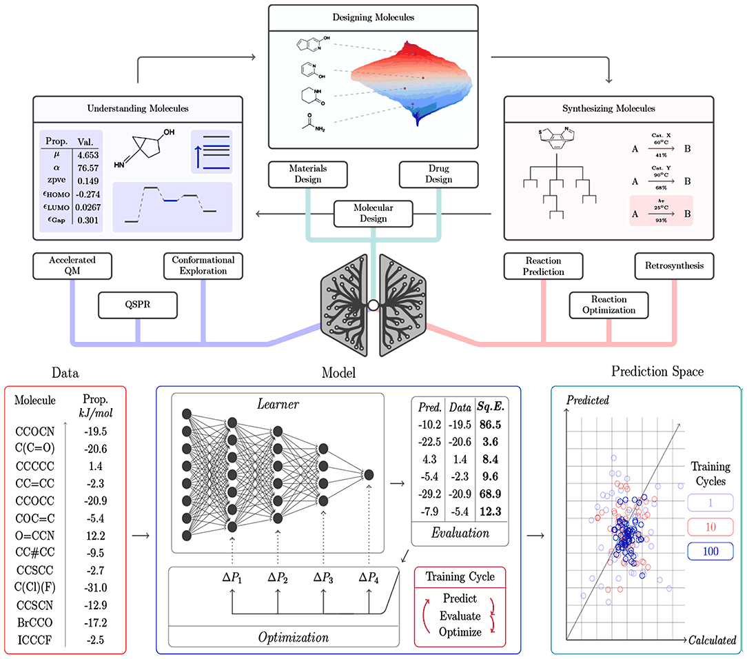
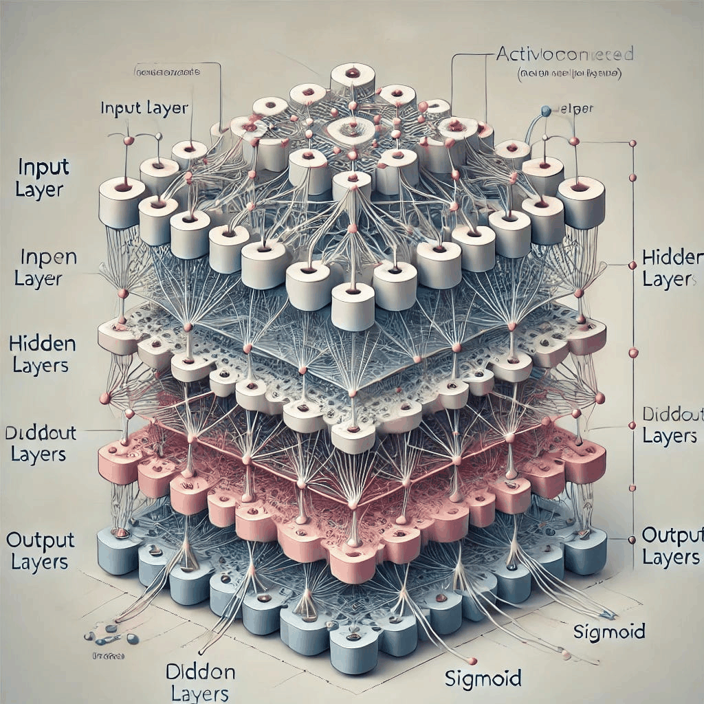
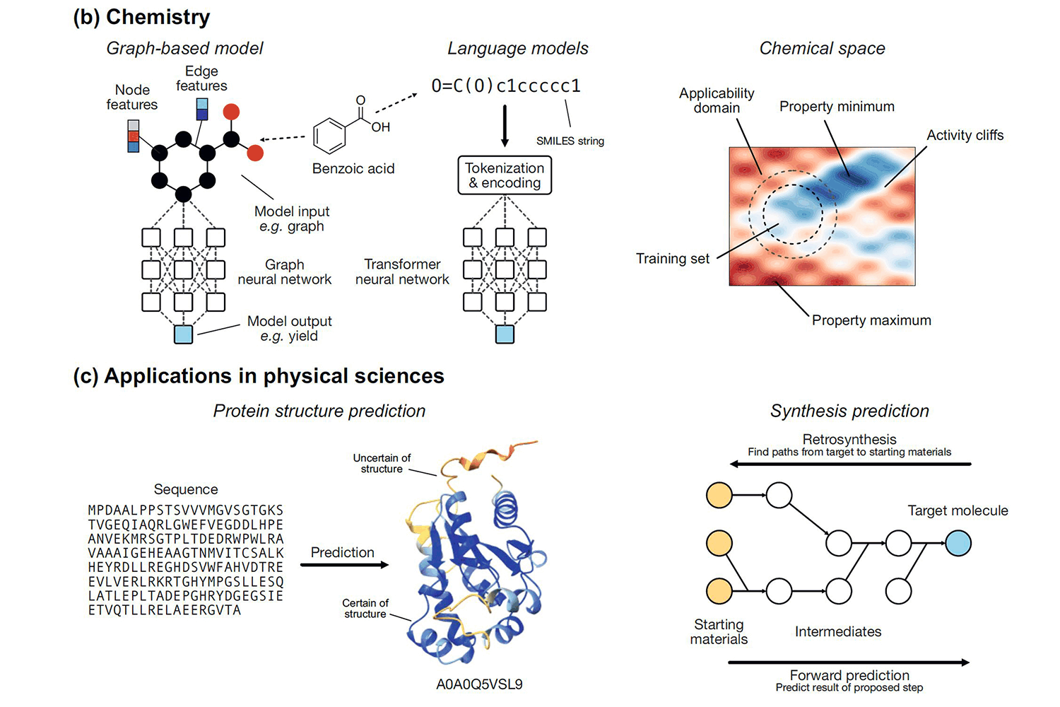
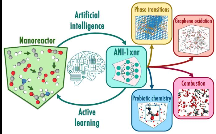
Deep Learning Execution Pipeline
(Preprocessing)
(Feature Extraction)
(Self-Attention)
(Loss Optimization)