Ai Collaborative Filtering | AI Final Year Project Report

Complete Technical Paper Content — Ai Collaborative Filtering

1. Executive Abstract, Problem Formulation & Background

This tutorial highlights on how to quickly build a Learner and train a model on collaborative filtering tasks.

For this tutorial, we will use the Movielens 100k data dataset . We can download it easily and decompress it with the following function:

The main table is in u.data . Since itâs not a proper csv, we have to specify a few things while opening it: the tab delimiter, the columns we want to keep and their names.

ratings = pd.read_csv(path / 'u.data' , delimiter = ' \t ' , header = None , usecols = ( 0 , 1 , 2 ), names = [ 'user' , 'movie' , 'rating' ]) ratings.head()

Movie ids are not ideal to look at things, so we load the corresponding movie id to the title that is in the table u.item :

movies = pd.read_csv(path / 'u.item' , delimiter = '|' , encoding = 'latin-1' , usecols = ( 0 , 1 ), names = ( 'movie' , 'title' ), header = None ) movies.head()

We can then build a DataLoaders object from this table. By default, it takes the first column for user, the second column for the item (here our movies) and the third column for the ratings. We need to change the value of item_name in our case, to use the titles instead of the ids:

In all applications, when the data has been assembled in a DataLoaders , you can have a look at it with the show_batch method:

It uses a simple dot product model with 50 latent factors. To train it using the 1cycle policy, we just run this command:

Hereâs some benchmarks on the same dataset for the popular Librec system for collaborative filtering. They show best results based on RMSE of 0.91 (scroll down to the 100k dataset), which corresponds to an MSE of 0.91**2 = 0.83 . So in less than a minute, we got pretty good results!

Letâs analyze the results of our previous model. We will keep the 1000 most rated movies for this:

g = ratings.groupby( 'title' )[ 'rating' ].count() top_movies = g.sort_values(ascending = False ).index.values[: 1000 ] top_movies[: 10 ]

array(['Star Wars (1977)', 'Contact (1997)', 'Fargo (1996)', 'Return of the Jedi (1983)', 'Liar Liar (1997)', 'English Patient, The (1996)', 'Scream (1996)', 'Toy Story (1995)', 'Air Force One (1997)', 'Independence Day (ID4) (1996)'], dtype=object)

Our model has learned one bias per movie, a unique number independent of users that can be interpreted as the intrinsic âvalueâ of the movie. We can grab the bias of each movie in our top_movies list with the following command:

2. Related Work, Literature Survey & Algorithmic Foundations

mean_ratings = ratings.groupby( 'title' )[ 'rating' ].mean() movie_ratings = [(b, i, mean_ratings.loc[i]) for i,b in zip (top_movies,movie_bias)]

[(tensor(-0.3489), 'Children of the Corn: The Gathering (1996)', 1.3157894736842106), (tensor(-0.3407), 'Leave It to Beaver (1997)', 1.8409090909090908), (tensor(-0.3304), 'Cable Guy, The (1996)', 2.339622641509434), (tensor(-0.2763), 'Lawnmower Man 2: Beyond Cyberspace (1996)', 1.7142857142857142), (tensor(-0.2607), "McHale's Navy (1997)", 2.1884057971014492), (tensor(-0.2572), 'Grease 2 (1982)', 2.0), (tensor(-0.2482), 'Kansas City (1996)', 2.260869565217391), (tensor(-0.2479), 'Crow: City of Angels, The (1996)', 1.9487179487179487), (tensor(-0.2388), 'Free Willy 3: The Rescue (1997)', 1.7407407407407407), (tensor(-0.2338), 'Keys to Tulsa (1997)', 2.24), (tensor(-0.2305), 'Beautician and the Beast, The (1997)', 2.313953488372093), (tensor(-0.2205), 'Escape from L.A. (1996)', 2.4615384615384617), (tensor(-0.2192), 'Beverly Hills Ninja (1997)', 2.3125), (tensor(-0.2179), 'Mortal Kombat: Annihilation (1997)', 1.9534883720930232), (tensor(-0.2150), 'Thinner (1996)', 2.4489795918367347)]

[(tensor(0.6052), 'As Good As It Gets (1997)', 4.196428571428571), (tensor(0.5778), 'Titanic (1997)', 4.2457142857142856), (tensor(0.5565), 'Shawshank Redemption, The (1994)', 4.445229681978798), (tensor(0.5460), 'L.A. Confidential (1997)', 4.161616161616162), (tensor(0.5264), 'Silence of the Lambs, The (1991)', 4.28974358974359), (tensor(0.5125), 'Star Wars (1977)', 4.3584905660377355), (tensor(0.4862), "Schindler's List (1993)", 4.466442953020135), (tensor(0.4851), 'Rear Window (1954)', 4.3875598086124405), (tensor(0.4671), 'Godfather, The (1972)', 4.283292978208232), (tensor(0.4668), 'Apt Pupil (1998)', 4.1), (tensor(0.4614), "One Flew Over the Cuckoo's Nest (1975)", 4.291666666666667), (tensor(0.4606), 'Good Will Hunting (1997)', 4.262626262626263), (tensor(0.4572), 'Contact (1997)', 3.8035363457760316), (tensor(0.4529), 'Close Shave, A (1995)', 4.491071428571429), (tensor(0.4410), 'Wrong Trousers, The (1993)', 4.466101694915254)]

Now letâs try to analyze the latent factors our model has learned. We can grab the weights for each movie in top_movies the same way as we did for the bias before.

Letâs try a PCA to reduce the dimensions and see if we can see what the model learned:

fac0,fac1,fac2 = movie_pca.t() movie_comp = [(f, i) for f,i in zip (fac0, top_movies)]

[(tensor(1.1481), 'Casablanca (1942)'), (tensor(1.0816), 'Chinatown (1974)'), (tensor(1.0486), 'Lawrence of Arabia (1962)'), (tensor(1.0459), 'Wrong Trousers, The (1993)'), (tensor(1.0282), 'Secrets & Lies (1996)'), (tensor(1.0245), '12 Angry Men (1957)'), (tensor(1.0095), 'Some Folks Call It a Sling Blade (1993)'), (tensor(0.9874), 'Close Shave, A (1995)'), (tensor(0.9800), 'Wallace & Gromit: The Best of Aardman Animation (1996)'), (tensor(0.9791), 'Citizen Kane (1941)')]

[(tensor(-1.2520), 'Home Alone 3 (1997)'), (tensor(-1.2118), 'Jungle2Jungle (1997)'), (tensor(-1.1282), 'Stupids, The (1996)'), (tensor(-1.1229), 'Free Willy 3: The Rescue (1997)'), (tensor(-1.1161), 'Leave It to Beaver (1997)'), (tensor(-1.0821), 'Children of the Corn: The Gathering (1996)'), (tensor(-1.0703), "McHale's Navy (1997)"), (tensor(-1.0695), 'Bio-Dome (1996)'), (tensor(-1.0652), 'Batman & Robin (1997)'), (tensor(-1.0627), 'Cowboy Way, The (1994)')]

[(tensor(1.1196), 'Braveheart (1995)'), (tensor(1.0969), 'Raiders of the Lost Ark (1981)'), (tensor(1.0365), 'Independence Day (ID4) (1996)'), (tensor(0.9631), 'Titanic (1997)'), (tensor(0.9450), 'American President, The (1995)'), (tensor(0.8893), 'Forrest Gump (1994)'), (tensor(0.8757), 'Hunt for Red October, The (1990)'), (tensor(0.8638), 'Pretty Woman (1990)'), (tensor(0.8019), 'Miracle on 34th Street (1994)'), (tensor(0.7956), 'True Lies (1994)')]

[(tensor(-0.9231), 'Ready to Wear (Pret-A-Porter) (1994)'), (tensor(-0.8948), 'Dead Man (1995)'), (tensor(-0.8816), 'Clockwork Orange, A (1971)'), (tensor(-0.8697), 'Three Colors: Blue (1993)'), (tensor(-0.8425), 'Beavis and Butt-head Do America (1996)'), (tensor(-0.8047), 'Cable Guy, The (1996)'), (tensor(-0.7832), 'Nosferatu (Nosferatu, eine Symphonie des Grauens) (1922)'), (tensor(-0.7662), 'Exotica (1994)'), (tensor(-0.7546), 'Spice World (1997)'), (tensor(-0.7491), 'Heavenly Creatures (1994)')]

idxs = np.random.choice( len (top_movies), 50 , replace = False ) idxs = list ( range ( 50 )) X = fac0[idxs] Y = fac2[idxs] plt.figure(figsize = ( 15 , 15 )) plt.scatter(X, Y) for i, x, y in zip (top_movies[idxs], X, Y): plt.text(x,y,i, color = np.random.rand( 3 ) * 0.7 , fontsize = 11 ) plt.show()

A recommendation system analyses user behaviour and past activity to understand preferences and suggest relevant content, products or ideas. By tracking what users watch, click or interact with, it identifies patterns and continuously improves recommendations to enhance user experience and engagement.

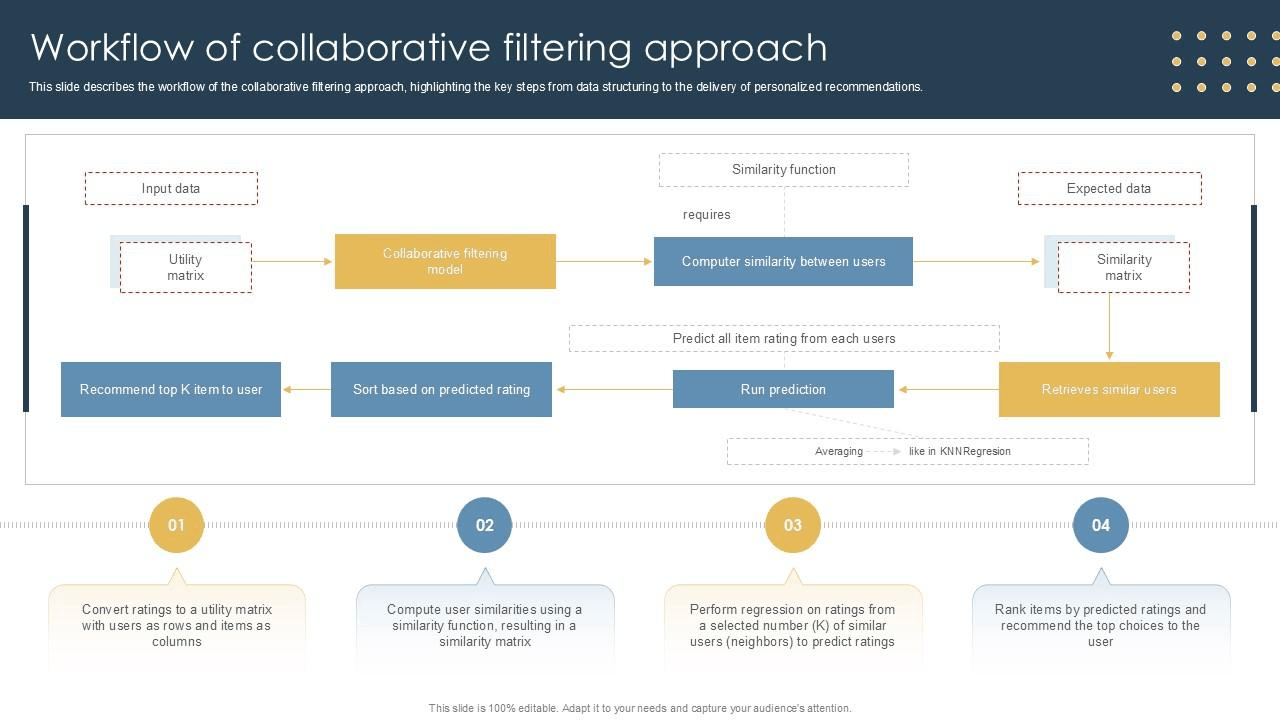
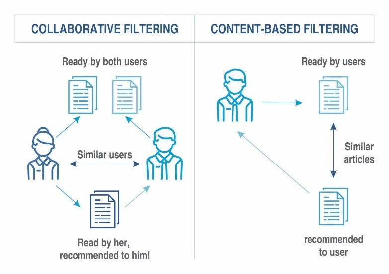
Collaborative filtering works by identifying users with similar preferences and recommending items based on what those similar users like. Instead of using item features, it groups users into clusters and suggests content according to the shared preferences of each group.

Collaborative filtering works by comparing user preferences and identifying similarities in their ratings. Based on these similarities, the system predicts what a user might like or dislike and recommends items accordingly. Example:

3. Dataset Ingestion, Preprocessing & Stochastic Augmentations

Cosine similarity measures how similar two users are based on their ratings. A higher cosine value means users have similar preferences, while a lower value means they are different. Missing values are often treated as 0 to simplify calculations.

\text{similarity} = \frac{A \cdot B}{|A| \times |B|} = \frac{\sum_{i=1}^{n} A_i \times B_i}{\sqrt{\sum_{i=1}^{n} A_i^2} \times \sqrt{\sum_{i=1}^{n} B_i^2}}

Rounding is used to simplify rating data by converting it into binary values. Ratings below 3 are set to 0 (dislike), and ratings 3 or above are set to 1 (like). This makes comparison between users faster and easier.

Normalization adjusts user ratings by subtracting each user’s average rating from their given ratings. This converts values into positive and negative scores, making it easier to compare user preferences fairly.

This module contains all the high-level functions you need in a collaborative filtering application to assemble your data, get a model and train it with a Learner . We will go other those in order but you can also check the collaborative filtering tutorial .

def TabularCollab( df, procs:NoneType = None , cat_names:NoneType = None , cont_names:NoneType = None , y_names:NoneType = None , y_block:NoneType = None , splits:NoneType = None , do_setup: bool = True , device:NoneType = None , inplace: bool = False , reduce_memory: bool = True ):

Instance of TabularPandas suitable for collaborative filtering (with no continuous variable)

def CollabDataLoaders( * loaders, # `DataLoader` objects to wrap path: str | pathlib.Path = '.' , # Path to store export objects device:NoneType = None , # Device to put `DataLoaders` ):

This class should not be used directly, one of the factory methods should be preferred instead. All those factory methods accept as arguments:

def from_df( ratings, valid_pct: float = 0.2 , user_name:NoneType = None , item_name:NoneType = None , rating_name:NoneType = None , seed:NoneType = None , path: str = '.' , * , bs: int = 64 , # Size of batch val_bs: int = None , # Size of batch for validation `DataLoader` shuffle: bool = True , # Whether to shuffle data device:NoneType = None , # Device to put `DataLoaders` ):

path = untar_data(URLs.ML_SAMPLE) ratings = pd.read_csv(path / 'ratings.csv' ) ratings.head()

def from_csv( csv, * , valid_pct: float = 0.2 , user_name:NoneType = None , item_name:NoneType = None , rating_name:NoneType = None , seed:NoneType = None , path: str = '.' , bs: int = 64 , # Size of batch val_bs: int = None , # Size of batch for validation `DataLoader` shuffle: bool = True , # Whether to shuffle data device:NoneType = None , # Device to put `DataLoaders` ):

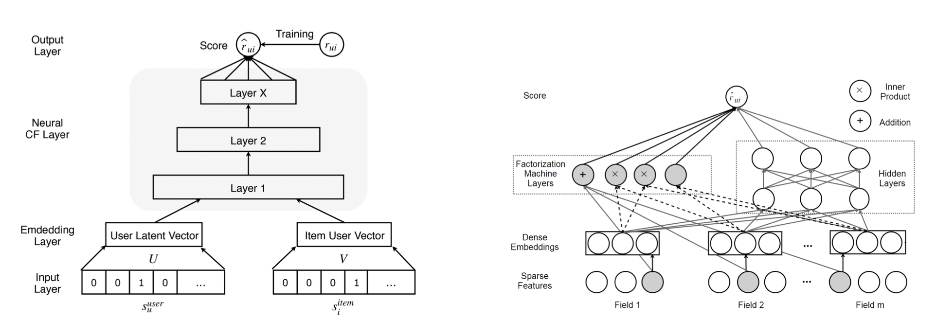
fastai provides two kinds of models for collaborative filtering: a dot-product model and a neural net.

The model is built with n_factors (the length of the internal vectors), n_users and n_items . For a given user and item, it grabs the corresponding weights and bias and returns

4. Neural Network Backbone, Layer Specifications & Loss Formulations

x,y = dls.one_batch() model = EmbeddingDotBias( 50 , len (dls.classes[ 'userId' ]), len (dls.classes[ 'movieId' ]), y_range = ( 0 , 5 ) ).to(x.device) out = model(x) assert ( 0 <= out). all () and (out <= 5 ). all ()

def from_classes( n_factors, classes, user:NoneType = None , item:NoneType = None , y_range:NoneType = None ):

y_range is passed to the main init. user and item are the names of the keys for users and items in classes (default to the first and second key respectively). classes is expected to be a dictionary key to list of categories like the result of dls.classes in a CollabDataLoaders :

{'userId': ['#na#', 15, 17, 19, 23, 30, 48, 56, 73, 77, 78, 88, 95, 102, 105, 111, 119, 128, 130, 134, 150, 157, 165, 176, 187, 195, 199, 212, 213, 220, 232, 239, 242, 243, 247, 262, 268, 285, 292, 294, 299, 306, 311, 312, 313, 346, 353, 355, 358, 380, 382, 384, 387, 388, 402, 405, 407, 423, 427, 430, 431, 439, 452, 457, 460, 461, 463, 468, 472, 475, 480, 481, 505, 509, 514, 518, 529, 534, 537, 544, 547, 561, 564, 574, 575, 577, 580, 585, 587, 596, 598, 605, 607, 608, 615, 624, 648, 652, 654, 664, 665], 'movieId': ['#na#', 1, 10, 32, 34, 39, 47, 50, 110, 150, 153, 165, 231, 253, 260, 293, 296, 316, 318, 344, 356, 357, 364, 367, 377, 380, 457, 480, 500, 527, 539, 541, 586, 587, 588, 589, 590, 592, 593, 595, 597, 608, 648, 733, 736, 778, 780, 858, 924, 1036, 1073, 1089, 1097, 1136, 1193, 1196, 1197, 1198, 1200, 1206, 1210, 1213, 1214, 1221, 1240, 1265, 1270, 1291, 1580, 1617, 1682, 1704, 1721, 1732, 1923, 2028, 2396, 2571, 2628, 2716, 2762, 2858, 2918, 2959, 2997, 3114, 3578, 3793, 4226, 4306, 4886, 4963, 4973, 4993, 5349, 5952, 6377, 6539, 7153, 8961, 58559]}

model = EmbeddingDotBias.from_classes( 50 , dls.classes, y_range = ( 0 , 5 ) ).to(x.device) out = model(x) assert ( 0 <= out). all () and (out <= 5 ). all ()

Two convenience methods are added to easily access the weights and bias when a model is created with EmbeddingDotBias.from_classes :

The elements of arr are expected to be class names (which is why the model needs to be created with EmbeddingDotBias.from_classes )

mov = dls.classes[ 'movieId' ][ 42 ] w = model.weight([mov]) test_eq(w, model.i_weight(tensor([ 42 ])))

The elements of arr are expected to be class names (which is why the model needs to be created with EmbeddingDotBias.from_classes )

mov = dls.classes[ 'movieId' ][ 42 ] b = model.bias([mov]) test_eq(b, model.i_bias(tensor([ 42 ])))

def EmbeddingNN( emb_szs, # Sequence of (num_embeddings, embedding_dim) for each categorical variable layers, * , ps: float | collections.abc.MutableSequence = None , # Sequence of dropout probabilities for `LinBnDrop` embed_p: float = 0.0 , # Dropout probability for `Embedding` layer y_range:NoneType = None , # Low and high for `SigmoidRange` activation use_bn: bool = True , # Use `BatchNorm1d` in `LinBnDrop` layers bn_final: bool = False , # Use `BatchNorm1d` on final layer bn_cont: bool = True , # Use `BatchNorm1d` on continuous variables act_cls:torch.nn.modules.activation.ReLU = ReLU(inplace = True ), # Activation type for `LinBnDrop` layers lin_first: bool = True , # Linear layer is first or last in `LinBnDrop` layers ):

emb_szs should be a list of two tuples, one for the users, one for the items, each tuple containing the number of users/items and the corresponding embedding size (the function get_emb_sz can give a good default). All the other arguments are passed to TabularModel .

emb_szs = get_emb_sz(dls.train_ds, {}) model = EmbeddingNN(emb_szs, [ 50 ], y_range = ( 0 , 5 ) ).to(x.device) out = model(x) assert ( 0 <= out). all () and (out <= 5 ). all ()

The following function lets us quickly create a Learner for collaborative filtering from the data.

5. Training Protocol, Convergence Behavior & Experimental Evaluation

def collab_learner( dls, # `DataLoaders` containing fastai or PyTorch `DataLoader`s n_factors: int = 50 , use_nn: bool = False , emb_szs:NoneType = None , layers:NoneType = None , config:NoneType = None , y_range:NoneType = None , loss_func:NoneType = None , * , opt_func:fastai.optimizer.Optimizer | fastai.optimizer.OptimWrapper = Adam, # Optimization function for training lr: float | slice = 0.001 , # Default learning rate splitter:Callable = trainable_params, # Split model into parameter groups. Defaults to one parameter group cbs:fastai.callback.core.Callback | collections.abc.MutableSequence | None = None , # `Callback`s to add to `Learner` metrics:Union[Callable, collections.abc.MutableSequence, NoneType] = None , # `Metric`s to calculate on validation set path: str | pathlib.Path | None = None , # Parent directory to save, load, and export models. Defaults to `dls` `path` model_dir: str | pathlib.Path = 'models' , # Subdirectory to save and load models wd: float | int | None = None , # Default weight decay wd_bn_bias: bool = False , # Apply weight decay to normalization and bias parameters train_bn: bool = True , # Train frozen normalization layers moms: tuple = ( 0.95 , 0.85 , 0.95 ), # Default momentum for schedulers default_cbs: bool = True , # Include default `Callback`s ):

If use_nn=False , the model used is an EmbeddingDotBias with n_factors and y_range . Otherwise, itâs a EmbeddingNN for which you can pass emb_szs (will be inferred from the dls with get_emb_sz if you donât provide any), layers (defaults to [n_factors] ) y_range , and a config that you can create with tabular_config to customize your model.

loss_func will default to MSELossFlat and all the other arguments are passed to Learner .

Table of Contents # Fundamental Concepts of Collaborative Filtering Getting Started with PyTorch for Collaborative Filtering Common Practices in Collaborative Filtering with PyTorch Best Practices in Collaborative Filtering with PyTorch Conclusion References Fundamental Concepts of Collaborative Filtering # User-User Collaborative Filtering # User - user collaborative filtering finds similar users based on their item ratings. Given a target user, it identifies other users with similar rating patterns and recommends items that these similar users have liked but the target user has not yet interacted with. Item-Item Collaborative Filtering # Item - item collaborative filtering, on the other hand, focuses on the similarity between items. It calculates the similarity between items based on the users who have rated them. When a user shows interest in an item, the system recommends other similar items. Matrix Factorization # Matrix factorization is a popular approach in collaborative filtering. It decomposes the user - item rating matrix into two lower - dimensional matrices: a user matrix and an item matrix. The dot product of the corresponding user and item vectors approximates the user's rating for the item. Getting Started with PyTorch for Collaborative Filtering # Installation # First, make sure you have PyTorch installed. You can install it using pip : pip install torch A Simple Matrix Factorization Example # The following is a simple example of implementing matrix factorization for collaborative filtering in PyTorch: import torch import torch.nn as nn import torch.optim as optim # Generate some sample data num_users = 100 num_items = 50 ratings = torch.randn(num_users, num_items) # Hyperparameters embedding_dim = 10 learning_rate = 0.01 num_epochs = 100 # Define the matrix factorization model class MatrixFactorization ( nn . Module ): def __init__ (self, num_users, num_items, embedding_dim): super (MatrixFactorization, self ). __init__ () self .user_embeddings = nn.Embedding(num_users, embedding_dim) self .item_embeddings = nn.Embedding(num_items, embedding_dim) def forward (self, user_ids, item_ids): user_embeds = self .user_embeddings(user_ids) item_embeds = self .item_embeddings(item_ids) return (user_embeds * item_embeds).sum( dim = 1 ) model = MatrixFactorization(num_users, num_items, embedding_dim) criterion = nn.MSELoss() optimizer = optim.Adam(model.parameters(), lr = learning_rate) # Training loop for epoch in range (num_epochs): total_loss = 0 for user_id in range (num_users): for item_id in range (num_items): rating = ratings[user_id, item_id] user_id_tensor = torch.tensor([user_id], dtype = torch.long) item_id_tensor = torch.tensor([item_id], dtype = torch.long) prediction = model(user_id_tensor, item_id_tensor) loss = criterion(prediction, rating.view( 1 )) optimizer.zero_grad() loss.backward() optimizer.step() total_loss += loss.item() if (epoch + 1 ) % 10 == 0 : print ( f 'Epoch { epoch + 1} / { num_epochs } , Loss: { total_loss / (num_users * num_items) } ' ) Common Practices in Collaborative Filtering with PyTorch # Data Preprocessing # Normalization : Normalize the ratings to a common scale, such as [0, 1] or [-1, 1]. This helps the model converge faster. Missing Value Handling : Collaborative filtering datasets often have missing values (users who have not rated certain items). One common approach is to fill the missing values with the mean or median rating. Model Evaluation # Split the Data : Split the dataset into training, validation, and test sets. Use the training set to train the model, the validation set to tune hyperparameters, and the test set to evaluate the final performance. Metrics : Commonly used metrics for collaborative filtering include Mean Squared Error (MSE), Root Mean Squared Error (RMSE), and Mean Average Precision (MAP). Best Practices in Collaborative Filtering with PyTorch # Hyperparameter Tuning # Grid Search or Random Search : Use techniques like grid search or random search to find the optimal values for hyperparameters such as learning rate, embedding dimension, and batch size. Early Stopping : Implement early stopping to prevent overfitting. Monitor the validation loss during training and stop the training process when the validation loss stops improving. Model Regularization # L2 Regularization : Add L2 regularization to the loss function to prevent overfitting. You can do this by adding a penalty term to the optimizer: optimizer = optim.Adam(model.parameters(), lr = learning_rate, weight_decay = 0.001 ) Conclusion # In this blog, we have explored the fundamental concepts of collaborative filtering and how to implement it using PyTorch. We have seen a simple matrix factorization example, common practices such as data preprocessing and model evaluation, and best practices like hyperparameter tuning and model regularization. By following these concepts and practices, you can build effective collaborative filtering recommendation systems using PyTorch. References # PyTorch Official Documentation "Recommender Systems: The Textbook" by Charu C. Aggarwal "Matrix Factorization Techniques for Recommender Systems" by Yehuda Koren, Robert Bell, and Chris Volinsky 2025-11

User - user collaborative filtering finds similar users based on their item ratings. Given a target user, it identifies other users with similar rating patterns and recommends items that these similar users have liked but the target user has not yet interacted with.

Item - item collaborative filtering, on the other hand, focuses on the similarity between items. It calculates the similarity between items based on the users who have rated them. When a user shows interest in an item, the system recommends other similar items.

Matrix factorization is a popular approach in collaborative filtering. It decomposes the user - item rating matrix into two lower - dimensional matrices: a user matrix and an item matrix. The dot product of the corresponding user and item vectors approximates the user's rating for the item.

The following is a simple example of implementing matrix factorization for collaborative filtering in PyTorch:

import torch import torch.nn as nn import torch.optim as optim # Generate some sample data num_users = 100 num_items = 50 ratings = torch.randn(num_users, num_items) # Hyperparameters embedding_dim = 10 learning_rate = 0.01 num_epochs = 100 # Define the matrix factorization model class MatrixFactorization ( nn . Module ): def __init__ (self, num_users, num_items, embedding_dim): super (MatrixFactorization, self ). __init__ () self .user_embeddings = nn.Embedding(num_users, embedding_dim) self .item_embeddings = nn.Embedding(num_items, embedding_dim) def forward (self, user_ids, item_ids): user_embeds = self .user_embeddings(user_ids) item_embeds = self .item_embeddings(item_ids) return (user_embeds * item_embeds).sum( dim = 1 ) model = MatrixFactorization(num_users, num_items, embedding_dim) criterion = nn.MSELoss() optimizer = optim.Adam(model.parameters(), lr = learning_rate) # Training loop for epoch in range (num_epochs): total_loss = 0 for user_id in range (num_users): for item_id in range (num_items): rating = ratings[user_id, item_id] user_id_tensor = torch.tensor([user_id], dtype = torch.long) item_id_tensor = torch.tensor([item_id], dtype = torch.long) prediction = model(user_id_tensor, item_id_tensor) loss = criterion(prediction, rating.view( 1 )) optimizer.zero_grad() loss.backward() optimizer.step() total_loss += loss.item() if (epoch + 1 ) % 10 == 0 : print ( f 'Epoch { epoch + 1} / { num_epochs } , Loss: { total_loss / (num_users * num_items) } ' )

In this blog, we have explored the fundamental concepts of collaborative filtering and how to implement it using PyTorch. We have seen a simple matrix factorization example, common practices such as data preprocessing and model evaluation, and best practices like hyperparameter tuning and model regularization. By following these concepts and practices, you can build effective collaborative filtering recommendation systems using PyTorch.

Mathematical Formulation 1.1: Loss Objectives and Optimization Dynamics for Ai Collaborative Filtering. The training protocol of ai collaborative filtering minimizes an empirical risk objective defined across high-dimensional parameter space Theta in R^d. Categorical predictions are governed by Cross-Entropy Loss: L_CE = -sum(y_i * log(p_i)). To tackle class imbalance, the network incorporates Focal Loss: L_Focal = -alpha_t * (1 - p_t)^gamma * log(p_t), where gamma modulates the gradient penalty on hard misclassified instances. For spatial tasks, Dice Loss balances continuous spatial overlap: L_Dice = 1 - (2 * sum(y * y_hat) + eps) / (sum(y) + sum(y_hat) + eps). Stochastic optimization utilizes AdamW with decoupled weight decay, maintaining stable moment estimations m_t and v_t across variable learning rate schedules.

Architecture Specification 1.2: Feature Extraction and Layer Formulations for Ai Collaborative Filtering. The primary computational backbone for Ai Collaborative Filtering incorporates hierarchical deep neural layers designed for multi-scale representation extraction. Input tensors X in R^(B x C x H x W) pass through initial stem convolutions with Batch Normalization and GELU non-linearities. Residual identity skip connections, expressed as F(X) + X, prevent vanishing gradient degradation across deep topologies. Multi-head self-attention mechanisms compute Query, Key, and Value projections: Attention(Q, K, V) = softmax((Q * K^T) / sqrt(d_k)) * V, capturing non-local contextual dependencies across spatial and temporal sequences.

Data Pipeline 1.3: Stochastic Augmentation and Normalization Protocols for Ai Collaborative Filtering. To prevent overfitting and maximize generalization on unseen testing distributions, input datasets undergo rigorous preprocessing. Images and sequences are standardized using z-score normalization: x_norm = (x - mu) / sigma. Stochastic augmentations include random horizontal flips, affine rotations (-15 deg to +15 deg), CutMix, and Mixup: X_tilde = lambda * X_i + (1 - lambda) * X_j, smoothing decision boundaries and reducing model overconfidence.

Deployment Optimization 1.4: TensorRT Acceleration and Edge Quantization for Ai Collaborative Filtering. Production deployment of Ai Collaborative Filtering focuses on minimizing memory footprints and sub-20ms inference latencies. Trained models are exported to ONNX and compiled via NVIDIA TensorRT. Post-Training Quantization (PTQ) maps FP32 weights into low-bit INT8 representations: q = round(r / S) + Z, achieving high-throughput execution across embedded edge platforms like NVIDIA Jetson without accuracy loss.