Complete Technical Paper Content — Ai Probabilistic Graphical Models
1. Executive Abstract, Problem Formulation & Background
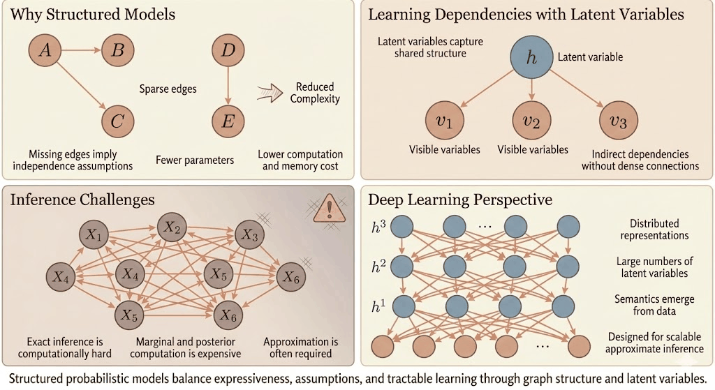
A graphical model or probabilistic graphical model (PGM) or structured probabilistic model is a probabilistic model for which a graph expresses the conditional dependence structure between random variables. Graphical models are commonly used in probability theory, statistics—particularly Bayesian statistics—and machine learning.
The undirected graph shown may have one of several interpretations; the common feature is that the presence of an edge implies some sort of dependence between the corresponding random variables. From this graph, we might deduce that B, C, and D are all conditionally independent given A. This means that if the value of A is known, then the values of B, C, and D provide no further information about each other. Equivalently (in this case), the joint probability distribution can be factorized as:
P [ A , B , C , D ] = f A B [ A , B ] ⋅ f A C [ A , C ] ⋅ f A D [ A , D ] {\displaystyle P[A,B,C,D]=f_{AB}[A,B]\cdot f_{AC}[A,C]\cdot f_{AD}[A,D]}
for some non-negative functions f A B , f A C , f A D {\displaystyle f_{AB},f_{AC},f_{AD}} .
If the network structure of the model is a directed acyclic graph, the model represents a factorization of the joint probability of all random variables. More precisely, if the events are X 1 , … , X n {\displaystyle X_{1},\ldots ,X_{n}} then the joint probability satisfies
P [ X 1 , … , X n ] = ∏ i = 1 n P [ X i | pa ( X i ) ] {\displaystyle P[X_{1},\ldots ,X_{n}]=\prod _{i=1}^{n}P[X_{i}|{\text{pa}}(X_{i})]}
where pa ( X i ) {\displaystyle {\text{pa}}(X_{i})} is the set of parents of node X i {\displaystyle X_{i}} (nodes with edges directed towards X i {\displaystyle X_{i}} ). In other words, the joint distribution factors into a product of conditional distributions. For example, in the directed acyclic graph shown in the Figure this factorization would be
P [ A , B , C , D ] = P [ A ] ⋅ P [ B | A ] ⋅ P [ C | A ] ⋅ P [ D | A , C ] {\displaystyle P[A,B,C,D]=P[A]\cdot P[B|A]\cdot P[C|A]\cdot P[D|A,C]} . Any two nodes are conditionally independent given the values of their parents. In general, any two sets of nodes are conditionally independent given a third set if a criterion called d-separation holds in the graph. Local independences and global independences are equivalent in Bayesian networks. This type of graphical model is known as a directed graphical model, Bayesian network, or belief network. Classic machine learning models like hidden Markov models, neural networks and newer models such as variable-order Markov models can be considered special cases of Bayesian networks. One of the simplest Bayesian Networks is the Naive Bayes classifier.
The next figure depicts a graphical model with a cycle. This may be interpreted in terms of each variable 'depending' on the values of its parents in some manner. The particular graph shown suggests a joint probability density that factors as
P [ A , B , C , D ] = P [ A ] ⋅ P [ B ] ⋅ P [ C , D | A , B ] {\displaystyle P[A,B,C,D]=P[A]\cdot P[B]\cdot P[C,D|A,B]} , but other interpretations are possible.
Targeted Bayesian network learning (TBNL) A factor graph is an undirected bipartite graph connecting variables and factors. Each factor represents a function over the variables it is connected to. This is a helpful representation for understanding and implementing belief propagation. A clique tree or junction tree is a tree of cliques, used in the junction tree algorithm. A chain graph is a graph which may have both directed and undirected edges, but without any directed cycles (i.e. if we start at any vertex and move along the graph respecting the directions of any arrows, we cannot return to the vertex we started from if we have passed an arrow). Both directed acyclic graphs and undirected graphs are special cases of chain graphs, which can therefore provide a way of unifying and generalizing Bayesian and Markov networks. An ancestral graph is a further extension, having directed, bidirected and undirected edges. Random field techniques A Markov random field, also known as a Markov network, is a model over an undirected graph. A graphical model with many repeated subunits can be represented with plate notation. A conditional random field is a discriminative model specified over an undirected graph. A restricted Boltzmann machine is a bipartite generative model specified over an undirected graph. A staged tree is an extension of a Bayesian network for sequences of discrete valued events. They allow for context specific independences and non-product sample spaces.
2. Related Work, Literature Survey & Algorithmic Foundations
In machine learning, diffusion models, also known as diffusion-based generative models or score-based generative models, are a class of latent variable generative models. A diffusion model consists of two major components: the forward diffusion process, and the reverse sampling process. The goal of diffusion models is to learn a diffusion process for a given dataset, such that the process can generate new elements that are distributed similarly as the original dataset. A diffusion model models data as generated by a diffusion process, whereby a new datum performs a random walk with drift through the space of all possible data. A trained diffusion model can be sampled in many ways, with different efficiency and quality. There are various equivalent formalisms, including Markov chains, denoising diffusion probabilistic models, noise conditioned score networks, and stochastic differential equations. They are typically trained using variational inference. The model responsible for denoising is typically called its "backbone". The backbone may be of any kind, but they are typically U-nets or transformers. As of 2024, diffusion models are mainly used for computer vision tasks, including image denoising, inpainting, super-resolution, image generation, and video generation. These typically involve training a neural network to sequentially denoise images corrupted by Gaussian noise. The model is trained to reverse the process of adding noise to an image. After training to convergence, it can be used for image generation by starting with an image composed of random noise, and applying the network iteratively to denoise the image. Diffusion-based image generators have seen widespread commercial interest, such as Stable Diffusion and DALL-E. These models typically combine diffusion models with other models, such as text-encoders and cross-attention modules to allow text-conditioned generation. Other than computer vision, diffusion models have also found applications in natural language processing such as text generation and summarization, sound generation, and reinforcement learning.
β 1 , . . . , β T ∈ ( 0 , 1 ) {\displaystyle \beta _{1},...,\beta _{T}\in (0,1)} are fixed constants.
α t := 1 − β t {\displaystyle \alpha _{t}:=1-\beta _{t}}
α ¯ t := α 1 ⋯ α t {\displaystyle {\bar {\alpha }}_{t}:=\alpha _{1}\cdots \alpha _{t}}
σ t := 1 − α ¯ t {\displaystyle \sigma _{t}:={\sqrt {1-{\bar {\alpha }}_{t}}}}
σ ~ t := σ t − 1 σ t β t {\displaystyle {\tilde {\sigma }}_{t}:={\frac {\sigma _{t-1}}{\sigma _{t}}}{\sqrt {\beta _{t}}}}
μ ~ t ( x t , x 0 ) := α t ( 1 − α ¯ t − 1 ) x t + α ¯ t − 1 ( 1 − α t ) x 0 σ t 2 {\displaystyle {\tilde {\mu }}_{t}(x_{t},x_{0}):={\frac {{\sqrt {\alpha _{t}}}(1-{\bar {\alpha }}_{t-1})x_{t}+{\sqrt {{\bar {\alpha }}_{t-1}}}(1-\alpha _{t})x_{0}}{\sigma _{t}^{2}}}}
N ( μ , Σ ) {\displaystyle {\mathcal {N}}(\mu ,\Sigma )} is the Gaussian distribution with mean μ {\displaystyle \mu } and variance Σ {\displaystyle \Sigma } , and N ( x | μ , Σ ) {\displaystyle {\mathcal {N}}(x|\mu ,\Sigma )} is the probability density at x {\displaystyle x} . A vertical bar denotes conditioning. A forward diffusion process starts at some starting point x 0 ∼ q {\displaystyle x_{0}\sim q} , where q {\displaystyle q} is the probability distribution to be learned, then repeatedly adds noise to it by x t = 1 − β t x t − 1 + β t z t {\displaystyle x_{t}={\sqrt {1-\beta _{t}}}x_{t-1}+{\sqrt {\beta _{t}}}z_{t}} where z 1 , . . . , z T {\displaystyle z_{1},...,z_{T}} are IID (Independent and identically distributed random variables) samples from N ( 0 , I ) {\displaystyle {\mathcal {N}}(0,I)} . The coefficients 1 − β t {\displaystyle {\sqrt {1-\beta _{t}}}} and β t {\displaystyle {\sqrt {\beta _{t}}}} ensure that Var ( X t ) = I {\displaystyle {\mbox{Var}}(X_{t})=I} assuming that Var ( X 0 ) = I {\displaystyle {\mbox{Var}}(X_{0})=I} . The values of β t {\displaystyle \beta _{t}} are chosen such that for any starting distribution of x 0 {\displaystyle x_{0}} , if it has finite second moment, then lim t → ∞ x t | x 0 {\displaystyle \lim _{t\to \infty }x_{t}|x_{0}} converges to N ( 0 , I ) {\displaystyle {\mathcal {N}}(0,I)} . The entire diffusion process then satisfies q ( x 0 : T ) = q ( x 0 ) q ( x 1 | x 0 ) ⋯ q ( x T | x T − 1 ) = q ( x 0 ) N ( x 1 | α 1 x 0 , β 1 I ) ⋯ N ( x T | α T x T − 1 , β T I ) {\displaystyle q(x_{0:T})=q(x_{0})q(x_{1}|x_{0})\cdots q(x_{T}|x_{T-1})=q(x_{0}){\mathcal {N}}(x_{1}|{\sqrt {\alpha _{1}}}x_{0},\beta _{1}I)\cdots {\mathcal {N}}(x_{T}|{\sqrt {\alpha _{T}}}x_{T-1},\beta _{T}I)} or ln q ( x 0 : T ) = ln q ( x 0 ) − ∑ t = 1 T 1 2 β t ‖ x t − 1 − β t x t − 1 ‖ 2 + C {\displaystyle \ln q(x_{0:T})=\ln q(x_{0})-\sum _{t=1}^{T}{\frac {1}{2\beta _{t}}}\|x_{t}-{\sqrt {1-\beta _{t}}}x_{t-1}\|^{2}+C} where C {\displaystyle C} is a normalization constant and often omitted. In particular, we note that x 1 : T | x 0 {\displaystyle x_{1:T}|x_{0}} is a Gaussian process, which affords us considerable freedom in reparameterization. For example, by standard manipulation with Gaussian process, x t | x 0 ∼ N ( α ¯ t x 0 , σ t 2 I ) {\displaystyle x_{t}|x_{0}\sim N\left({\sqrt {{\bar {\alpha }}_{t}}}x_{0},\sigma _{t}^{2}I\right)}
x t − 1 | x t , x 0 ∼ N ( μ ~ t ( x t , x 0 ) , σ ~ t 2 I ) {\displaystyle x_{t-1}|x_{t},x_{0}\sim {\mathcal {N}}({\tilde {\mu }}_{t}(x_{t},x_{0}),{\tilde {\sigma }}_{t}^{2}I)} In particular, notice that for large t {\displaystyle t} , the variable x t | x 0 ∼ N ( α ¯ t x 0 , σ t 2 I ) {\displaystyle x_{t}|x_{0}\sim N\left({\sqrt {{\bar {\alpha }}_{t}}}x_{0},\sigma _{t}^{2}I\right)} converges to N ( 0 , I ) {\displaystyle {\mathcal {N}}(0,I)} . That is, after a long enough diffusion process, we end up with some x T {\displaystyle x_{T}} that is very close to N ( 0 , I ) {\displaystyle {\mathcal {N}}(0,I)} , with all traces of the original x 0 ∼ q {\displaystyle x_{0}\sim q} gone. For example, since x t | x 0 ∼ N ( α ¯ t x 0 , σ t 2 I ) {\displaystyle x_{t}|x_{0}\sim N\left({\sqrt {{\bar {\alpha }}_{t}}}x_{0},\sigma _{t}^{2}I\right)} we can sample x t | x 0 {\displaystyle x_{t}|x_{0}} directly "in one step", instead of going through all the intermediate steps x 1 , x 2 , . . . , x t − 1 {\displaystyle x_{1},x_{2},...,x_{t-1}} .
p θ ( x t − 1 | x t ) = N ( x t − 1 | μ θ ( x t , t ) , Σ θ ( x t , t ) ) {\displaystyle p_{\theta }(x_{t-1}|x_{t})={\mathcal {N}}(x_{t-1}|\mu _{\theta }(x_{t},t),\Sigma _{\theta }(x_{t},t))} The goal now is to learn the parameters θ {\displaystyle \theta } such that p θ ( x 0 ) {\displaystyle p_{\theta }(x_{0})} is as close to q ( x 0 ) {\displaystyle q(x_{0})} as possible. To do that, we use maximum likelihood estimation with variational inference.
Compute the noise estimate ϵ ← ϵ θ ( x t , t ) {\displaystyle \epsilon \leftarrow \epsilon _{\theta }(x_{t},t)}
3. Dataset Ingestion, Preprocessing & Stochastic Augmentations
Compute the original data estimate x ~ 0 ← ( x t − σ t ϵ ) / α ¯ t {\displaystyle {\tilde {x}}_{0}\leftarrow (x_{t}-\sigma _{t}\epsilon )/{\sqrt {{\bar {\alpha }}_{t}}}}
Sample the previous data x t − 1 ∼ N ( μ ~ t ( x t , x ~ 0 ) , σ ~ t 2 I ) {\displaystyle x_{t-1}\sim {\mathcal {N}}({\tilde {\mu }}_{t}(x_{t},{\tilde {x}}_{0}),{\tilde {\sigma }}_{t}^{2}I)}
Change time t ← t − 1 {\displaystyle t\leftarrow t-1}
One, we no longer need to normalize q ( x ) {\displaystyle q(x)} , but can use any q ~ ( x ) = C q ( x ) {\displaystyle {\tilde {q}}(x)=Cq(x)} , where C = ∫ q ~ ( x ) d x > 0 {\displaystyle C=\int {\tilde {q}}(x)dx>0} is any unknown constant that is of no concern to us. Two, we are comparing q ( x ) {\displaystyle q(x)} neighbors q ( x + d x ) {\displaystyle q(x+dx)} , by q ( x ) q ( x + d x ) = e − ⟨ ∇ x ln q , d x ⟩ {\displaystyle {\frac {q(x)}{q(x+dx)}}=e^{-\langle \nabla _{x}\ln q,dx\rangle }}
Let the score function be s ( x ) := ∇ x ln q ( x ) {\displaystyle s(x):=\nabla _{x}\ln q(x)} ; then consider what we can do with s ( x ) {\displaystyle s(x)} . As it turns out, s ( x ) {\displaystyle s(x)} allows us to sample from q ( x ) {\displaystyle q(x)} using thermodynamics. Specifically, if we have a potential energy function U ( x ) = − ln q ( x ) {\displaystyle U(x)=-\ln q(x)} , and a lot of particles in the potential well, then the distribution at thermodynamic equilibrium is the Boltzmann distribution q U ( x ) ∝ e − U ( x ) / k B T = q ( x ) 1 / k B T {\displaystyle q_{U}(x)\propto e^{-U(x)/k_{B}T}=q(x)^{1/k_{B}T}} . At temperature k B T = 1 {\displaystyle k_{B}T=1} , the Boltzmann distribution is exactly q ( x ) {\displaystyle q(x)} . Therefore, to model q ( x ) {\displaystyle q(x)} , we may start with a particle sampled at any convenient distribution (such as the standard Gaussian distribution), then simulate the motion of the particle forwards according to the Langevin equation
d x t = − ∇ x t U ( x t ) d t + d W t {\displaystyle dx_{t}=-\nabla _{x_{t}}U(x_{t})dt+dW_{t}}
and the Boltzmann distribution is, by Fokker-Planck equation, the unique thermodynamic equilibrium. So no matter what distribution x 0 {\displaystyle x_{0}} has, the distribution of x t {\displaystyle x_{t}} converges in distribution to q {\displaystyle q} as t → ∞ {\displaystyle t\to \infty } .
d y t = 1 2 β ( T − t ) y t d t + β ( T − t ) ∇ y t ln ρ T − t ( y t ) ⏟ score function d t + β ( T − t ) d W t {\displaystyle dy_{t}={\frac {1}{2}}\beta (T-t)y_{t}dt+\beta (T-t)\underbrace {\nabla _{y_{t}}\ln \rho _{T-t}\left(y_{t}\right)} _{\text{score function }}dt+{\sqrt {\beta (T-t)}}dW_{t}}
then by plugging into the Fokker-Planck equation, we find that ∂ t ρ T − t = ∂ t ν t {\displaystyle \partial _{t}\rho _{T-t}=\partial _{t}\nu _{t}} . Thus this cloud of points is the original cloud, evolving backwards.
α ¯ t = ( 1 − β 1 ) ⋯ ( 1 − β t ) = e ∑ i ln ( 1 − β i ) → e − ∫ 0 t β ( t ) d t {\displaystyle {\bar {\alpha }}_{t}=(1-\beta _{1})\cdots (1-\beta _{t})=e^{\sum _{i}\ln(1-\beta _{i})}\to e^{-\int _{0}^{t}\beta (t)dt}}
x t | x 0 ∼ N ( e − 1 2 ∫ 0 t β ( t ) d t x 0 , ( 1 − e − ∫ 0 t β ( t ) d t ) I ) {\displaystyle x_{t}|x_{0}\sim N\left(e^{-{\frac {1}{2}}\int _{0}^{t}\beta (t)dt}x_{0},\left(1-e^{-\int _{0}^{t}\beta (t)dt}\right)I\right)}
4. Neural Network Backbone, Layer Specifications & Loss Formulations
In particular, we see that we can directly sample from any point in the continuous diffusion process without going through the intermediate steps, by first sampling x 0 ∼ q , z ∼ N ( 0 , I ) {\displaystyle x_{0}\sim q,z\sim {\mathcal {N}}(0,I)} , then get x t = e − 1 2 ∫ 0 t β ( t ) d t x 0 + ( 1 − e − ∫ 0 t β ( t ) d t ) z {\displaystyle x_{t}=e^{-{\frac {1}{2}}\int _{0}^{t}\beta (t)dt}x_{0}+\left(1-e^{-\int _{0}^{t}\beta (t)dt}\right)z} . That is, we can quickly sample x t ∼ ρ t {\displaystyle x_{t}\sim \rho _{t}} for any t ≥ 0 {\displaystyle t\geq 0} . Now, define a certain probability distribution γ {\displaystyle \gamma } over [ 0 , ∞ ) {\displaystyle [0,\infty )} , then the score-matching loss function is defined as the expected Fisher divergence:
L ( θ ) = E t ∼ γ , x t ∼ ρ t [ ‖ f θ ( x t , t ) ‖ 2 + 2 ∇ ⋅ f θ ( x t , t ) ] {\displaystyle L(\theta )=E_{t\sim \gamma ,x_{t}\sim \rho _{t}}[\|f_{\theta }(x_{t},t)\|^{2}+2\nabla \cdot f_{\theta }(x_{t},t)]}
After training, f θ ( x t , t ) ≈ ∇ ln ρ t {\displaystyle f_{\theta }(x_{t},t)\approx \nabla \ln \rho _{t}} , so we can perform the backwards diffusion process by first sampling x T ∼ N ( 0 , I ) {\displaystyle x_{T}\sim {\mathcal {N}}(0,I)} , then integrating the SDE from t = T {\displaystyle t=T} to t = 0 {\displaystyle t=0} :
x t − d t = x t + 1 2 β ( t ) x t d t + β ( t ) f θ ( x t , t ) d t + β ( t ) d W t {\displaystyle x_{t-dt}=x_{t}+{\frac {1}{2}}\beta (t)x_{t}dt+\beta (t)f_{\theta }(x_{t},t)dt+{\sqrt {\beta (t)}}dW_{t}}
This may be done by any SDE integration method, such as Euler–Maruyama method. The name "noise conditional score network" is explained thus:
"network", because f θ {\displaystyle f_{\theta }} is implemented as a neural network. "score", because the output of the network is interpreted as approximating the score function ∇ ln ρ t {\displaystyle \nabla \ln \rho _{t}} . "noise conditional", because ρ t {\displaystyle \rho _{t}} is equal to ρ 0 {\displaystyle \rho _{0}} blurred by an added Gaussian noise that increases with time, and so the score function depends on the amount of noise added.
∇ x t ln q ( x t ) = 1 σ t 2 ( − x t + α ¯ t E q [ x 0 | x t ] ) {\displaystyle \nabla _{x_{t}}\ln q(x_{t})={\frac {1}{\sigma _{t}^{2}}}(-x_{t}+{\sqrt {{\bar {\alpha }}_{t}}}E_{q}[x_{0}|x_{t}])}
As described previously, the DDPM loss function is ∑ t L s i m p l e , t {\displaystyle \sum _{t}L_{simple,t}} with
L s i m p l e , t = E x 0 ∼ q ; z ∼ N ( 0 , I ) [ ‖ ϵ θ ( x t , t ) − z ‖ 2 ] {\displaystyle L_{simple,t}=E_{x_{0}\sim q;z\sim {\mathcal {N}}(0,I)}\left[\left\|\epsilon _{\theta }(x_{t},t)-z\right\|^{2}\right]}
where x t = α ¯ t x 0 + σ t z {\displaystyle x_{t}={\sqrt {{\bar {\alpha }}_{t}}}x_{0}+\sigma _{t}z} . By a change of variables,
L s i m p l e , t = E x 0 , x t ∼ q [ ‖ ϵ θ ( x t , t ) − x t − α ¯ t x 0 σ t ‖ 2 ] = E x t ∼ q , x 0 ∼ q ( ⋅ | x t ) [ ‖ ϵ θ ( x t , t ) − x t − α ¯ t x 0 σ t ‖ 2 ] {\displaystyle L_{simple,t}=E_{x_{0},x_{t}\sim q}\left[\left\|\epsilon _{\theta }(x_{t},t)-{\frac {x_{t}-{\sqrt {{\bar {\alpha }}_{t}}}x_{0}}{\sigma _{t}}}\right\|^{2}\right]=E_{x_{t}\sim q,x_{0}\sim q(\cdot |x_{t})}\left[\left\|\epsilon _{\theta }(x_{t},t)-{\frac {x_{t}-{\sqrt {{\bar {\alpha }}_{t}}}x_{0}}{\sigma _{t}}}\right\|^{2}\right]}
5. Training Protocol, Convergence Behavior & Experimental Evaluation
and the term inside becomes a least squares regression, so if the network actually reaches the global minimum of loss, then we have ϵ θ ( x t , t ) = x t − α ¯ t E q [ x 0 | x t ] σ t = − σ t ∇ x t ln q ( x t ) {\displaystyle \epsilon _{\theta }(x_{t},t)={\frac {x_{t}-{\sqrt {{\bar {\alpha }}_{t}}}E_{q}[x_{0}|x_{t}]}{\sigma _{t}}}=-\sigma _{t}\nabla _{x_{t}}\ln q(x_{t})}
Thus, given a good score-based network, its predicted score is a good prediction of the noise (after scaling by σ t {\displaystyle \sigma _{t}} ), and thus can be used for denoising. Conversely, the continuous limit x t − 1 = x t − d t , β t = β ( t ) d t , z t d t = d W t {\displaystyle x_{t-1}=x_{t-dt},\beta _{t}=\beta (t)dt,z_{t}{\sqrt {dt}}=dW_{t}} of the backward equation
x t − 1 = x t α t − β t σ t α t ϵ θ ( x t , t ) + β t z t ; z t ∼ N ( 0 , I ) {\displaystyle x_{t-1}={\frac {x_{t}}{\sqrt {\alpha _{t}}}}-{\frac {\beta _{t}}{\sigma _{t}{\sqrt {\alpha _{t}}}}}\epsilon _{\theta }(x_{t},t)+{\sqrt {\beta _{t}}}z_{t};\quad z_{t}\sim {\mathcal {N}}(0,I)}
x t − d t = x t ( 1 + β ( t ) d t / 2 ) + β ( t ) ∇ x t ln q ( x t ) d t + β ( t ) d W t {\displaystyle x_{t-dt}=x_{t}(1+\beta (t)dt/2)+\beta (t)\nabla _{x_{t}}\ln q(x_{t})dt+{\sqrt {\beta (t)}}dW_{t}} Thus, at infinitesimal steps of DDPM, a denoising network performs score-based diffusion.
In DDPM, the sequence of numbers 0 = σ 0 < σ 1 < ⋯ < σ T < 1 {\displaystyle 0=\sigma _{0}<\sigma _{1}<\cdots <\sigma _{T}<1} is called a (discrete time) noise schedule. In general, consider a strictly increasing monotonic function σ {\displaystyle \sigma } of type R → ( 0 , 1 ) {\displaystyle \mathbb {R} \to (0,1)} , such as the sigmoid function. In that case, a noise schedule is a sequence of real numbers λ 1 < λ 2 < ⋯ < λ T {\displaystyle \lambda _{1}<\lambda _{2}<\cdots <\lambda _{T}} . It then defines a sequence of noises σ t := σ ( λ t ) {\displaystyle \sigma _{t}:=\sigma (\lambda _{t})} , which then derives the other quantities β t = 1 − 1 − σ t 2 1 − σ t − 1 2 {\displaystyle \beta _{t}=1-{\frac {1-\sigma _{t}^{2}}{1-\sigma _{t-1}^{2}}}} . In order to use arbitrary noise schedules, instead of training a noise prediction model ϵ θ ( x t , t ) {\displaystyle \epsilon _{\theta }(x_{t},t)} , one trains ϵ θ ( x t , σ t ) {\displaystyle \epsilon _{\theta }(x_{t},\sigma _{t})} . Similarly, for the noise conditional score network, instead of training f θ ( x t , t ) {\displaystyle f_{\theta }(x_{t},t)} , one trains f θ ( x t , σ t ) {\displaystyle f_{\theta }(x_{t},\sigma _{t})} .
Since the diffusion model is a general method for modelling probability distributions, if one wants to model a distribution over images, one can first encode the images into a lower-dimensional space by an encoder, then use a diffusion model to model the distribution over encoded images. Then to generate an image, one can sample from the diffusion model, then use a decoder to decode it into an image. The encoder-decoder pair is most often a variational autoencoder (VAE).
p ( x | y ) ∝ p ( y | x ) p ( x ) {\displaystyle p(x|y)\propto p(y|x)p(x)}
in other words, if we have a good model of the space of all images, and a good image-to-class translator, we get a class-to-image translator "for free". In the equation for backward diffusion, the score ∇ ln p ( x ) {\displaystyle \nabla \ln p(x)} can be replaced by
∇ x ln p ( x | y ) = ∇ x ln p ( x ) ⏟ score + ∇ x ln p ( y | x ) ⏟ classifier guidance {\displaystyle \nabla _{x}\ln p(x|y)=\underbrace {\nabla _{x}\ln p(x)} _{\text{score}}+\underbrace {\nabla _{x}\ln p(y|x)} _{\text{classifier guidance}}}
where ∇ x ln p ( x ) {\displaystyle \nabla _{x}\ln p(x)} is the score function, trained as previously described, and ∇ x ln p ( y | x ) {\displaystyle \nabla _{x}\ln p(y|x)} is found by using a differentiable image classifier. During the diffusion process, we need to condition on the time, giving ∇ x t ln p ( x t | y , t ) = ∇ x t ln p ( y | x t , t ) + ∇ x t ln p ( x t | t ) {\displaystyle \nabla _{x_{t}}\ln p(x_{t}|y,t)=\nabla _{x_{t}}\ln p(y|x_{t},t)+\nabla _{x_{t}}\ln p(x_{t}|t)} Although, usually the classifier model does not depend on time, in which case p ( y | x t , t ) = p ( y | x t ) {\displaystyle p(y|x_{t},t)=p(y|x_{t})} . Classifier guidance is defined for the gradient of score function, thus for score-based diffusion network, but as previously noted, score-based diffusion models are equivalent to denoising models by ϵ θ ( x t , t ) = − σ t ∇ x t ln p ( x t | t ) {\displaystyle \epsilon _{\theta }(x_{t},t)=-\sigma _{t}\nabla _{x_{t}}\ln p(x_{t}|t)} , and similarly, ϵ θ ( x t , y , t ) = − σ t ∇ x t ln p ( x t | y , t ) {\displaystyle \epsilon _{\theta }(x_{t},y,t)=-\sigma _{t}\nabla _{x_{t}}\ln p(x_{t}|y,t)} . Therefore, classifier guidance works for denoising diffusion as well, using the modified noise prediction: ϵ θ ( x t , y , t ) = ϵ θ ( x t , t ) − σ t ∇ x t ln p ( y | x t , t ) ⏟ classifier guidance {\displaystyle \epsilon _{\theta }(x_{t},y,t)=\epsilon _{\theta }(x_{t},t)-\underbrace {\sigma _{t}\nabla _{x_{t}}\ln p(y|x_{t},t)} _{\text{classifier guidance}}}
p γ ( x | y ) ∝ p ( y | x ) γ p ( x ) {\displaystyle p_{\gamma }(x|y)\propto p(y|x)^{\gamma }p(x)}
Model Figures & Evaluation Curves (4 Images)
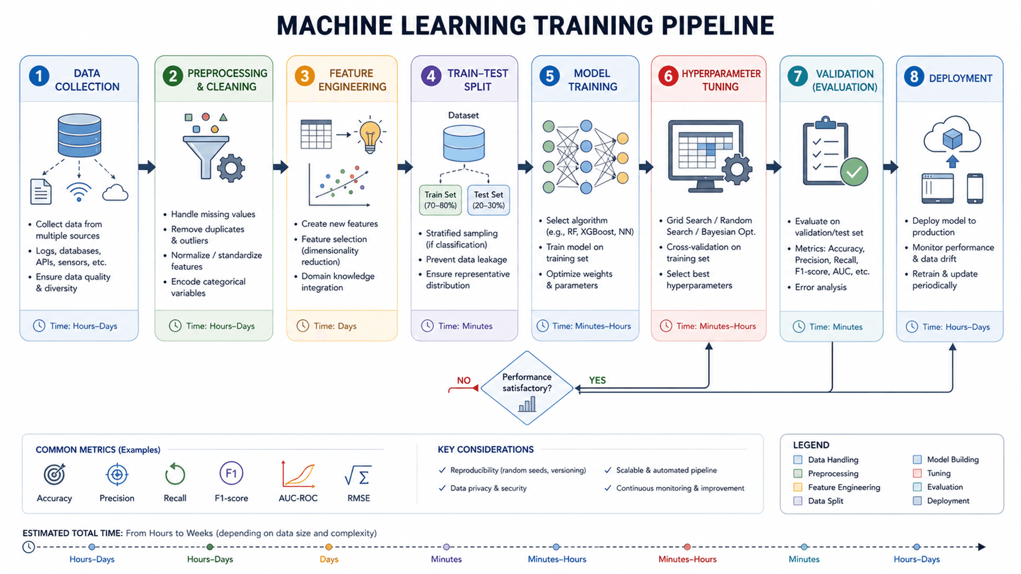
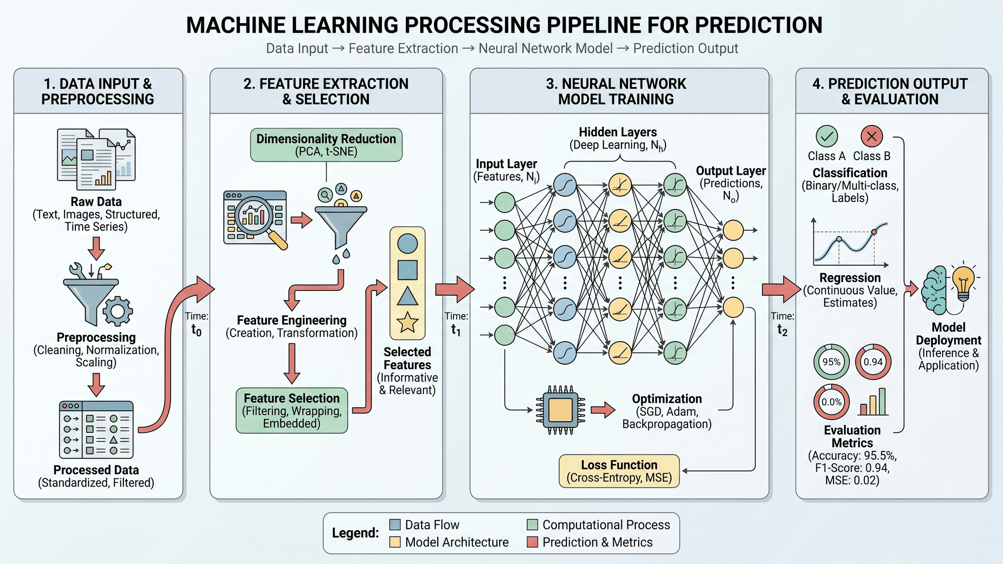
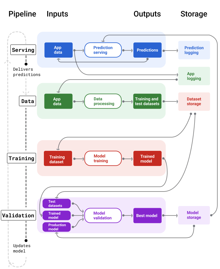
Deep Learning Execution Pipeline
(Preprocessing)
(Feature Extraction)
(Self-Attention)
(Loss Optimization)