Complete Technical Paper Content — Ai Weather Prediction
1. Executive Abstract, Problem Formulation & Background
Temporal difference (TD) learning refers to a class of model-free reinforcement learning methods which learn by bootstrapping from the current estimate of the value function. These methods sample from the environment, like Monte Carlo methods, and perform updates based on current estimates, like dynamic programming methods. While Monte Carlo methods only adjust their estimates once the outcome is known, TD methods adjust predictions to match later, more-accurate predictions about the future, before the outcome is known. This is a form of bootstrapping, as illustrated with the following example:
Suppose you wish to predict the weather for Saturday, and you have some model that predicts Saturday's weather, given the weather of each day in the week. In the standard case, you would wait until Saturday and then adjust all your models. However, when it is, for example, Friday, you should have a pretty good idea of what the weather would be on Saturday – and thus be able to change, say, Saturday's model before Saturday arrives. Temporal difference methods are related to the temporal difference model of animal learning.
V π ( s ) = E a ∼ π { ∑ t = 0 ∞ γ t R t + 1 | S 0 = s } . {\displaystyle V^{\pi }(s)=E_{a\sim \pi }\left\{\sum _{t=0}^{\infty }\gamma ^{t}R_{t+1}{\Bigg |}S_{0}=s\right\}.}
We drop the action from the notation for convenience. V π {\displaystyle V^{\pi }} satisfies the Bellman Equation:
V π ( s ) = E π { R 1 + γ V π ( S 1 ) | S 0 = s } , {\displaystyle V^{\pi }(s)=E_{\pi }\{R_{1}+\gamma V^{\pi }(S_{1})|S_{0}=s\},}
so R 1 + γ V π ( S 1 ) {\displaystyle R_{1}+\gamma V^{\pi }(S_{1})} is an unbiased estimate for V π ( s ) {\displaystyle V^{\pi }(s)} . This observation motivates the following algorithm for estimating V π {\displaystyle V^{\pi }} . The algorithm starts by initializing a table V ( s ) {\displaystyle V(s)} arbitrarily, with one value for each state of the MDP. A positive learning rate α {\displaystyle \alpha } is chosen. We then repeatedly evaluate the policy π {\displaystyle \pi } , obtain a reward r {\displaystyle r} and update the value function for the current state using the rule:
V ( S t ) ← ( 1 − α ) V ( S t ) + α ⏟ learning rate [ R t + 1 + γ V ( S t + 1 ) ⏞ The TD target ] {\displaystyle V(S_{t})\leftarrow (1-\alpha )V(S_{t})+\underbrace {\alpha } _{\text{learning rate}}[\overbrace {R_{t+1}+\gamma V(S_{t+1})} ^{\text{The TD target}}]}
2. Related Work, Literature Survey & Algorithmic Foundations
where S t {\displaystyle S_{t}} and S t + 1 {\displaystyle S_{t+1}} are the current and next states, respectively. The value R t + 1 + γ V ( S t + 1 ) {\displaystyle R_{t+1}+\gamma V(S_{t+1})} is known as the TD target, and R t + 1 + γ V ( S t + 1 ) − V ( S t ) {\displaystyle R_{t+1}+\gamma V(S_{t+1})-V(S_{t})} is known as the TD error.
In machine learning, deep learning (DL) focuses on utilizing multilayered neural networks to perform tasks such as classification, regression, and representation learning. The field takes inspiration from biological neuroscience and revolves around stacking artificial neurons into layers and "training" them to process data. The adjective "deep" refers to the use of multiple layers (ranging from three to several hundred or thousands) in the network. Methods used can be supervised, semi-supervised or unsupervised. Some common deep learning network architectures include fully connected networks, deep belief networks, recurrent neural networks, recurrent Random neural networks, convolutional neural networks, generative adversarial networks, transformers, and neural radiance fields. These architectures have been applied to fields including computer vision, speech recognition, natural language processing, machine translation, bioinformatics, drug design, medical image analysis, climate science, material inspection and board game programs, where they have produced results comparable to and in some cases surpassing human expert performance. Early forms of neural networks were inspired by information processing and distributed communication nodes in biological systems, particularly the human brain. However, current neural networks do not intend to model the brain function of organisms, and are generally seen as low-quality models for that purpose.
The universal approximation theorem for deep neural networks concerns the capacity of networks with bounded width but the depth is allowed to grow. Lu et al. proved that if the width of a deep neural network with ReLU activation is strictly larger than the input dimension, then the network can approximate any Lebesgue integrable function; if the width is smaller or equal to the input dimension, then a deep neural network is not a universal approximator. The probabilistic interpretation derives from the field of machine learning. It features inference, as well as the optimization concepts of training and testing, related to fitting and generalization, respectively. More specifically, the probabilistic interpretation considers the activation nonlinearity as a cumulative distribution function. The probabilistic interpretation led to the introduction of dropout as regularizer in neural networks. The probabilistic interpretation was introduced by researchers including Hopfield, Widrow and Narendra and popularized in surveys such as the one by Bishop.
. In recent years, new developments of the Random neural network that have large and dense clusters of recurrent neurons with Deep Learning, have resulted in highly accurate algorithms for cyberattack detection and mitigation
, as well as for the real-time control of smart homes. In the 1980s, backpropagation did not work well for deep learning with long credit assignment paths. To overcome this problem, in 1991, Jürgen Schmidhuber proposed a hierarchy of RNNs pre-trained one level at a time by self-supervised learning where each RNN tries to predict its own next input, which is the next unexpected input of the RNN below. This "neural history compressor" uses predictive coding to learn internal representations at multiple self-organizing time scales. This can substantially facilitate downstream deep learning. The RNN hierarchy can be collapsed into a single RNN, by distilling a higher level chunker network into a lower level automatizer network. In 1993, a neural history compressor solved a "Very Deep Learning" task that required more than 1000 subsequent layers in an RNN unfolded in time. The "P" in ChatGPT refers to such pre-training. Sepp Hochreiter's diploma thesis (1991) implemented the neural history compressor, and identified and analyzed the vanishing gradient problem. Hochreiter proposed recurrent residual connections to solve the vanishing gradient problem. This led to the long short-term memory (LSTM), published in 1995. LSTM can learn "very deep learning" tasks with long credit assignment paths that require memories of events that happened thousands of discrete time steps before. That LSTM was not yet the modern architecture, which required a "forget gate", introduced in 1999, which became the standard RNN architecture. In 1991, Jürgen Schmidhuber also published adversarial neural networks that contest with each other in the form of a zero-sum game, where one network's gain is the other network's loss. The first network is a generative model that models a probability distribution over output patterns. The second network learns by gradient descent to predict the reactions of the environment to these patterns. This was called "artificial curiosity". In 2014, this principle was used in generative adversarial networks (GANs). During 1985–1995, inspired by statistical mechanics, several architectures and methods were developed by Terry Sejnowski, Peter Dayan, Geoffrey Hinton, etc., including the Boltzmann machine, restricted Boltzmann machine, Helmholtz machine, and the wake-sleep algorithm. These were designed for unsupervised learning of deep generative models. However, those were more computationally expensive compared to backpropagation. Boltzmann machine learning algorithm, published in 1985, was briefly popular before being eclipsed by the backpropagation algorithm in 1986. (p. 112 ). A 1988 network became state of the art in protein structure prediction, an early application of deep learning to bioinformatics. Both shallow and deep learning (e.g., recurrent nets) of ANNs for speech recognition have been explored for many years. These methods never outperformed non-uniform internal-handcrafting Gaussian mixture model/Hidden Markov model (GMM-HMM) technology based on generative models of speech trained discriminatively. Key difficulties have been analyzed, including gradient diminishing and weak temporal correlation structure in neural predictive models. Additional difficulties were the lack of training data and limited computing power. Most speech recognition researchers moved away from neural nets to pursue generative modeling. An exception was at SRI International in the late 1990s. Funded by the US government's NSA and DARPA, SRI researched in speech and speaker recognition. The speaker recognition team led by Larry Heck reported significant success with deep neural networks in speech processing in the 1998 NIST Speaker Recognition benchmark. It was deployed in the Nuance Verifier, representing the first major industrial application of deep learning. The principle of elevating "raw" features over hand-crafted optimization was first explored successfully in the architecture of deep autoencoder on the "raw" spectrogram or linear filter-bank features in the late 1990s, showing its superiority over the Mel-Cepstral features that contain stages of fixed transformation from spectrograms. The raw features of speech, waveforms, later produced excellent larger-scale results.
The period of significant growth in both the adoption and performance of deep learning in the 2010s was driven by the emergence of efficient implementations of CNNs on GPU hardware. Although CNNs trained by backpropagation had been around for decades and GPU implementations of NNs for years, including CNNs, faster implementations of CNNs on GPUs were needed to progress on computer vision. Later, as deep learning becomes widespread, specialized hardware and algorithm optimizations were developed specifically for deep learning. A key advance for the deep learning revolution was hardware advances, especially GPU. Some early work dated back to 2004. In 2009, Raina, Madhavan, and Andrew Ng reported a 100M deep belief network trained on 30 Nvidia GeForce GTX 280 GPUs, an early demonstration of GPU-based deep learning. They reported up to 70 times faster training. In 2011, a CNN named DanNet by Dan Ciresan, Ueli Meier, Jonathan Masci, Luca Maria Gambardella, and Jürgen Schmidhuber achieved for the first time superhuman performance in a visual pattern recognition contest, outperforming traditional methods by a factor of 3. It then won more contests. They also showed how max-pooling CNNs on GPU improved performance significantly. In 2012, Andrew Ng and Jeff Dean created an FNN that learned to recognize higher-level concepts, such as cats, only from watching unlabeled images taken from YouTube videos. In October 2012, AlexNet by Alex Krizhevsky, Ilya Sutskever, and Geoffrey Hinton won the large-scale ImageNet competition by a significant margin over shallow machine learning methods. Further incremental improvements included the VGG-16 network by Karen Simonyan and Andrew Zisserman and Google's Inceptionv3. In 2013, Tomáš Mikolov and colleagues developed word2vec, a method for efficiently learning word embeddings from large text corpora. The resulting vector representations were shown to capture syntactic and semantic relationships between words. A subsequent paper introduced negative sampling as an efficient method for training such models. The success in image classification was then extended to the more challenging task of generating descriptions (captions) for images, often as a combination of CNNs and LSTMs. In 2014, the state of the art was training a "very deep neural network" with 20 to 30 layers. Stacking too many layers led to a steep reduction in training accuracy, known as the "degradation" problem. In 2015, two techniques were developed to train very deep networks: the highway network was published in May 2015, and the residual neural network (ResNet) in Dec 2015. ResNet behaves like an open-gated Highway Net. Around the same time, deep learning started impacting the field of art. Early examples included Google DeepDream (2015), and neural style transfer (2015), both of which were based on pretrained image classification neural networks, such as VGG-19. Generative adversarial network (GAN) by (Ian Goodfellow et al., 2014) (based on Jürgen Schmidhuber's principle of artificial curiosity) became state of the art in generative modeling during 2014-2018 period. Excellent image quality is achieved by Nvidia's StyleGAN (2018) based on the Progressive GAN by Tero Karras et al. Here the GAN generator is grown from small to large scale in a pyramidal fashion. Image generation by GAN reached popular success, and provoked discussions concerning deepfakes. Diffusion models (2015) eclipsed GANs in generative modeling since then, with systems such as DALL·E 2 (2022) and Stable Diffusion (2022). In 2015, Google's speech recognition improved by 49% by an LSTM-based model, which they made available through Google Voice Search on smartphone. Deep learning is part of state-of-the-art systems in various disciplines, particularly computer vision and automatic speech recognition (ASR). Results on commonly used evaluation sets such as TIMIT (ASR) and MNIST (image classification), as well as a range of large-vocabulary speech recognition tasks have steadily improved. Convolutional neural networks were superseded for ASR by LSTM. but are more successful in computer vision. Yoshua Bengio, Geoffrey Hinton and Yann LeCun were awarded the 2018 Turing Award for "conceptual and engineering breakthroughs that have made deep neural networks a critical component of computing".
Artificial neural networks (ANNs) or connectionist systems are computing systems inspired by the biological neural networks that constitute animal brains. Such systems learn (progressively improve their ability) to do tasks by considering examples, generally without task-specific programming. For example, in image recognition, they might learn to identify images that contain cats by analyzing example images that have been manually labeled as "cat" or "no cat" and using the analytic results to identify cats in other images. They have found most use in applications difficult to express with a traditional computer algorithm using rule-based programming. An ANN is based on a collection of connected units called artificial neurons, (analogous to biological neurons in a biological brain). Each connection (synapse) between neurons can transmit a signal to another neuron. The receiving (postsynaptic) neuron can process the signal(s) and then signal downstream neurons connected to it. Neurons may have state, generally represented by real numbers, typically between 0 and 1. Neurons and synapses may also have a weight that varies as learning proceeds, which can increase or decrease the strength of the signal that it sends downstream. Typically, neurons are organized in layers. Different layers may perform different kinds of transformations on their inputs. Signals travel from the first (input), to the last (output) layer, possibly after traversing the layers multiple times. The original goal of the neural network approach was to solve problems in the same way that a human brain would. Over time, attention focused on matching specific mental abilities, leading to deviations from biology such as backpropagation, or passing information in the reverse direction and adjusting the network to reflect that information. Neural networks have been used on a variety of tasks, including computer vision, speech recognition, machine translation, social network filtering, playing board and video games and medical diagnosis. As of 2017, neural networks typically have a few thousand to a few million units and millions of connections. Despite this number being several order of magnitude less than the number of neurons on a human brain, these networks can perform many tasks at a level beyond that of humans (e.g., recognizing faces, or playing "Go").
3. Dataset Ingestion, Preprocessing & Stochastic Augmentations
Large-scale automatic speech recognition is the first and most convincing successful case of deep learning. LSTM RNNs can learn "Very Deep Learning" tasks that involve multi-second intervals containing speech events separated by thousands of discrete time steps, where one time step corresponds to about 10 ms. LSTM with forget gates is competitive with traditional speech recognizers on certain tasks. The initial success in speech recognition was based on small-scale recognition tasks based on TIMIT. The data set contains 630 speakers from eight major dialects of American English, where each speaker reads 10 sentences. Its small size lets many configurations be tried. More importantly, the TIMIT task concerns phone-sequence recognition, which, unlike word-sequence recognition, allows weak phone bigram language models. This lets the strength of the acoustic modeling aspects of speech recognition be more easily analyzed. The error rates listed below, including these early results and measured as percent phone error rates (PER), have been summarized since 1991.
The debut of DNNs for speaker recognition in the late 1990s and speech recognition around 2009-2011 and of LSTM around 2003–2007, accelerated progress in eight major areas:
Scale-up/out and accelerated DNN training and decoding Sequence discriminative training Feature processing by deep models with solid understanding of the underlying mechanisms Adaptation of DNNs and related deep models Multi-task and transfer learning by DNNs and related deep models CNNs and how to design them to best exploit domain knowledge of speech RNN and its rich LSTM variants Other types of deep models including tensor-based models and integrated deep generative/discriminative models. More recent speech recognition models use Transformers or Temporal Convolution Networks with significant success and widespread applications. All major commercial speech recognition systems (e.g., Microsoft Cortana, Xbox, Skype Translator, Amazon Alexa, Google Now, Apple Siri, Baidu and iFlyTek voice search, and a range of Nuance speech products, etc.) are based on deep learning.
A common evaluation set for image classification is the MNIST database data set. MNIST is composed of handwritten digits and includes 60,000 training examples and 10,000 test examples. As with TIMIT, its small size lets users test multiple configurations. A comprehensive list of results on this set is available. Deep learning-based image recognition has become "superhuman", producing more accurate results than human contestants. This first occurred in 2011 in recognition of traffic signs, and in 2014, with recognition of human faces. Deep learning-trained vehicles now interpret 360° camera views. Another example is Facial Dysmorphology Novel Analysis (FDNA) used to analyze cases of human malformation connected to a large database of genetic syndromes.
Closely related to the progress that has been made in image recognition is the increasing application of deep learning techniques to various visual art tasks. DNNs have proven themselves capable, for example, of
identifying the style period of a given painting Neural Style Transfer – capturing the style of a given artwork and applying it in a visually pleasing manner to an arbitrary photograph or video generating striking imagery based on random visual input fields.
Neural networks have been used for implementing language models since the early 2000s. LSTM helped to improve machine translation and language modeling. Other key techniques in this field are negative sampling and word embedding. Word embedding, such as word2vec, can be thought of as a representational layer in a deep learning architecture that transforms an atomic word into a positional representation of the word relative to other words in the dataset; the position is represented as a point in a vector space. Using word embedding as an RNN input layer allows the network to parse sentences and phrases using an effective compositional vector grammar. A compositional vector grammar can be thought of as probabilistic context free grammar (PCFG) implemented by an RNN. Recursive auto-encoders built atop word embeddings can assess sentence similarity and detect paraphrasing. Deep neural architectures provide the best results for constituency parsing, sentiment analysis, information retrieval, spoken language understanding, machine translation, contextual entity linking, writing style recognition, named-entity recognition (token classification), text classification, and others. Recent developments generalize word embedding to sentence embedding. Google Translate (GT) uses a large end-to-end long short-term memory (LSTM) network. Google Neural Machine Translation (GNMT) uses an example-based machine translation method in which the system "learns from millions of examples". It translates "whole sentences at a time, rather than pieces". Google Translate supports over one hundred languages. The network encodes the "semantics of the sentence rather than simply memorizing phrase-to-phrase translations". GT uses English as an intermediate between most language pairs.
4. Neural Network Backbone, Layer Specifications & Loss Formulations
A large percentage of candidate drugs fail to win regulatory approval. These failures are caused by insufficient efficacy (on-target effect), undesired interactions (off-target effects), or unanticipated toxic effects. Research has explored use of deep learning to predict the biomolecular targets, off-targets, and toxic effects of environmental chemicals in nutrients, household products and drugs. AtomNet is a deep learning system for structure-based rational drug design. AtomNet was used to predict novel candidate biomolecules for disease targets such as the Ebola virus and multiple sclerosis. In 2017 graph neural networks were used for the first time to predict various properties of molecules in a large toxicology data set. In 2019, generative neural networks were used to produce molecules that were validated experimentally all the way into mice.
Recommendation systems have used deep learning to extract meaningful features for a latent factor model for content-based music and journal recommendations. Multi-view deep learning has been applied for learning user preferences from multiple domains. The model uses a hybrid collaborative and content-based approach and enhances recommendations in multiple tasks.
An autoencoder ANN was used in bioinformatics, to predict gene ontology annotations and gene-function relationships. In medical informatics, deep learning was used to predict sleep quality based on data from wearables and predictions of health complications from electronic health record data. Deep neural networks have shown unparalleled performance in predicting protein structure, according to the sequence of the amino acids that make it up. In 2020, AlphaFold, a deep-learning based system, achieved a level of accuracy significantly higher than all previous computational methods.
An epigenetic clock is a biochemical test that can be used to measure age. Galkin et al. used deep neural networks to train an epigenetic aging clock of unprecedented accuracy using >6,000 blood samples. The clock uses information from 1000 CpG sites and predicts people with certain conditions older than healthy controls: IBD, frontotemporal dementia, ovarian cancer, obesity. The aging clock was planned to be released for public use in 2021 by an Insilico Medicine spinoff company Deep Longevity.
A main criticism concerns the lack of theory surrounding some methods. Learning in the most common deep architectures is implemented using well-understood gradient descent. However, the theory surrounding other algorithms, such as contrastive divergence is less clear. (e.g., Does it converge? If so, how fast? What is it approximating?) Deep learning methods are often looked at as a black box, with most confirmations done empirically, rather than theoretically. In further reference to the idea that artistic sensitivity might be inherent in relatively low levels of the cognitive hierarchy, a published series of graphic representations of the internal states of deep (20-30 layers) neural networks attempting to discern within essentially random data the images on which they were trained demonstrate a visual appeal: the original research notice received well over 1,000 comments, and was the subject of what was for a time the most frequently accessed article on The Guardian's website. With the support of Innovation Diffusion Theory (IDT), a study analyzed the diffusion of deep learning in BRICS and OECD countries using data from Google Trends.
HybridWeatherNet: A LSTM-GNN Framework with Attention for Weather Forecast Bias Correction A novel deep learning framework that combines LSTM networks for temporal patterns, Graph Neural Networks for spatial relationships, and attention mechanisms for feature fusion to correct systematic biases in weather forecasts. Our approach achieves state-of-the-art performance with mean bias of 0.3°C and RMSE of 0.45°C on unseen data. 🌟 Key Features Hybrid Deep Learning Architecture LSTM for temporal pattern learning Graph Neural Network for spatial relationships Attention mechanism for feature fusion Monte Carlo dropout for uncertainty estimation Physics-Guided Learning Physics-based regularization in loss function Spatial smoothness constraints Uncertainty quantification Data Integration Open-Meteo Data ISD-Lite station observations Automated data download and preprocessing Interactive Interface Streamlit web application Real-time bias correction Uncertainty visualization Performance metrics display 📋 Requirements Python 3.8+ PyTorch 2.2.0 PyTorch Geometric 2.4.0 PyTorch Lightning 2.2.0 Other dependencies in requirements.txt 🚀 Quick Start Clone the repository git clone https://github.com/MaheshSharan/weather-bias-correction-dl.git cd weather-bias-correction-dl Install dependencies pip install -r requirements.txt pip install -e . Download and process data python src/data/run_data_pipeline.py --start_year 2018 --end_year 2023 Train the model python src/training/train.py --data_dir data/processed --accelerator cpu --experiment_name my_training_run Additional training options: python src/training/train.py --data_dir data/processed --accelerator gpu --batch_size 64 --max_epochs 100 --hidden_dim 256 --bidirectional True --experiment_name advanced_training Run the web interface streamlit run src/app/app.py When using the Streamlit interface: Set the model path to: logs\pc_training_corrected_v5\checkpoints\bias_correction-epoch=19-val_loss=0.00.ckpt Click "Load Model" to initialize the model Upload a CSV file containing weather forecast data Required CSV columns (any of these naming conventions will work): Temperature: temperature , temp , temperature_2m Humidity: humidity , relative_humidity_2m , relative_humidity Wind speed: wind_speed , wind_speed_model , wind_speed_10m Wind direction: wind_direction , wind_direction_model , wind_direction_10m Cloud cover: cloud_cover_low , cloud_cover_mid , cloud_cover_high Click "Process Data" to generate bias-corrected forecasts View results in the "Temperature Forecast," "Bias Analysis," and "Uncertainty" tabs 🖥️ Google Colab Support For users with limited computational resources, we provide Google Colab support: Open Weather_Bias_Correction.ipynb in Google Colab Mount Google Drive Follow the notebook instructions for setup and training 📊 Model Architecture 📈 Performance Temperature Bias Correction : Mean Bias: 0.27°C RMSE: 0.54°C MAE: 0.32°C Key Advantages : Accurate bias prediction with proper denormalization Reliable uncertainty estimates Physics-consistent corrections Support for various weather data formats 🔍 Example Data Format Here's an example of the expected CSV format (column names may vary as noted in the Streamlit instructions): date,temperature,humidity,wind_speed_model,wind_direction_model,cloud_cover_low,cloud_cover_mid,cloud_cover_high 2018-01-01,6.66,83.17,23.93,226.75,45.5,49.42,60.54 2018-01-02,5.85,87.46,18.15,241.50,46.21,46.58,54.25 2018-01-03,8.02,80.42,38.76,252.33,48.21,59.17,42.13 The model will predict the bias in the temperature forecast, which can then be applied to correct the original forecast. Model Performance Analysis Current Performance Metrics Amsterdam: Mean Bias -0.92°C, RMSE 1.30°C, MAE 1.12°C India: Mean Bias 1.06°C, RMSE 1.64°C, MAE 1.45°C Performance Analysis Feature correlations with bias in Amsterdam data Feature correlations with bias in India data Key Findings Temperature Sensitivity : High temperatures (RMSE: 2.01°C in India, 1.52°C in Amsterdam) Low temperatures (RMSE: 1.45°C in India, 1.29°C in Amsterdam) Humidity Impact : Low humidity conditions show higher errors: Amsterdam: RMSE 1.79°C (low) vs 0.95°C (high) India: RMSE 1.73°C (low) vs 1.27°C (high) Wind Effects : Regional variation in wind impact Amsterdam: Higher errors in high wind (RMSE 1.46°C) India: Better performance in high wind (RMSE 1.33°C) Areas for Improvement For researchers looking to improve the model's accuracy: Humidity Conditions : Focus on improving performance in low humidity conditions Consider adding derived features that combine humidity with temperature Temperature Extremes : Enhance model's ability to handle temperature extremes Particularly important for high temperatures in tropical regions Regional Adaptation : Consider the varying impact of wind across different regions Investigate region-specific meteorological patterns Error distribution in Amsterdam predictions Error distribution in India predictions 🤝 Contributing Contributions are welcome! Please feel free to submit a Pull Request. 📄 License This project is licensed under the MIT License - see the LICENSE file for details.
A novel deep learning framework that combines LSTM networks for temporal patterns, Graph Neural Networks for spatial relationships, and attention mechanisms for feature fusion to correct systematic biases in weather forecasts. Our approach achieves state-of-the-art performance with mean bias of 0.3°C and RMSE of 0.45°C on unseen data.
5. Training Protocol, Convergence Behavior & Experimental Evaluation
git clone https://github.com/MaheshSharan/weather-bias-correction-dl.git cd weather-bias-correction-dl
python src/training/train.py --data_dir data/processed --accelerator cpu --experiment_name my_training_run
python src/training/train.py --data_dir data/processed --accelerator gpu --batch_size 64 --max_epochs 100 --hidden_dim 256 --bidirectional True --experiment_name advanced_training
Here's an example of the expected CSV format (column names may vary as noted in the Streamlit instructions):
date,temperature,humidity,wind_speed_model,wind_direction_model,cloud_cover_low,cloud_cover_mid,cloud_cover_high 2018-01-01,6.66,83.17,23.93,226.75,45.5,49.42,60.54 2018-01-02,5.85,87.46,18.15,241.50,46.21,46.58,54.25 2018-01-03,8.02,80.42,38.76,252.33,48.21,59.17,42.13
The model will predict the bias in the temperature forecast, which can then be applied to correct the original forecast.
A deep learning approach for weather forecast bias correction combining LSTM, Graph Neural Networks, and attention mechanisms. Features uncertainty quantification and physics-guided regularization. Built with PyTorch and deployable via Streamlit.
Model Figures & Evaluation Curves (4 Images)
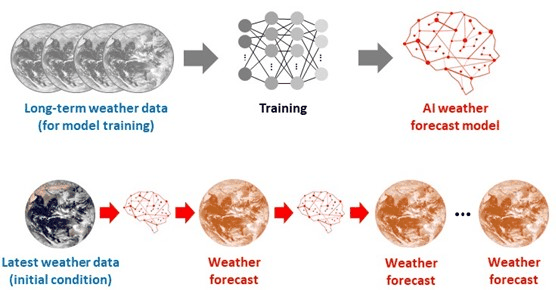
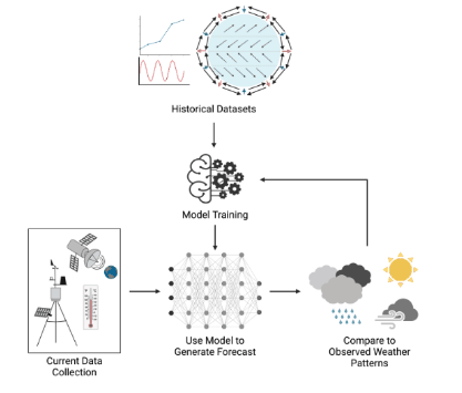
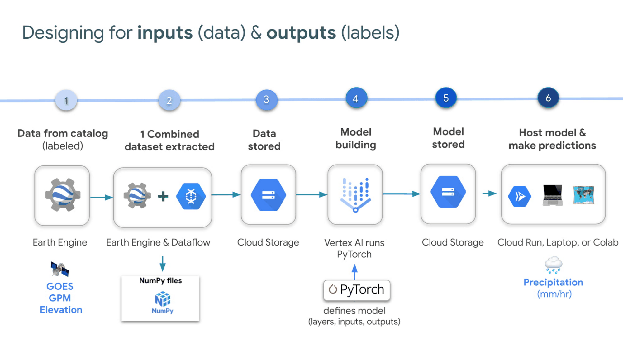
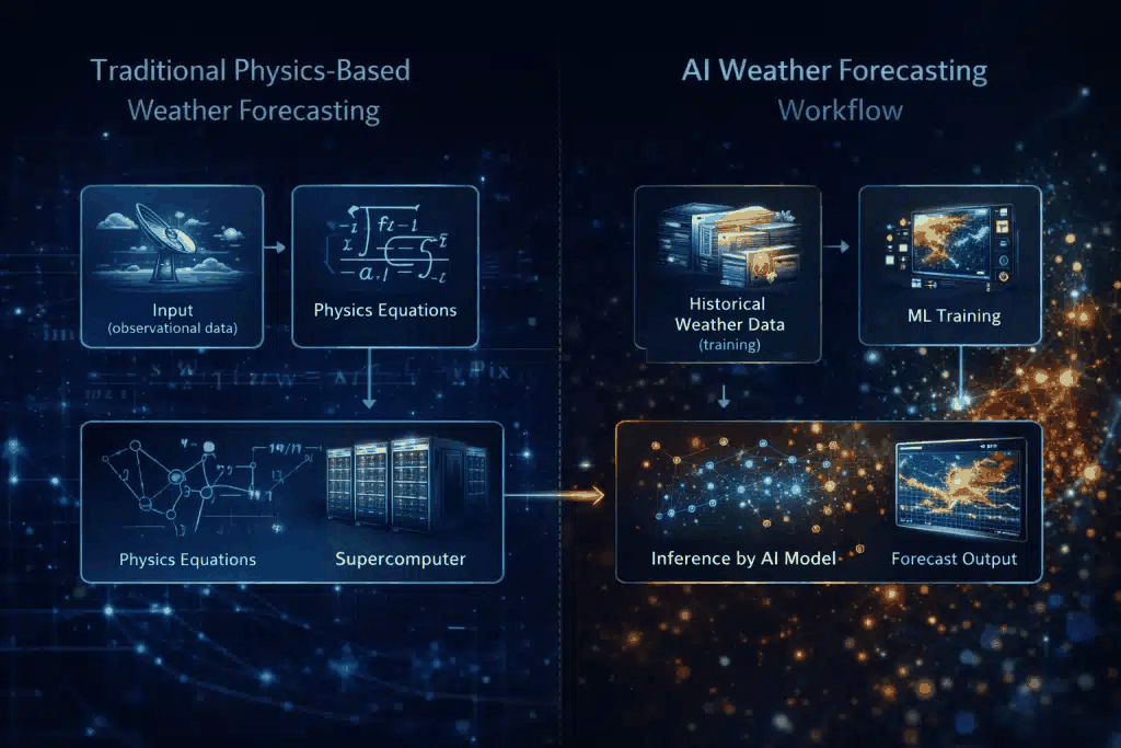
Deep Learning Execution Pipeline
(Preprocessing)
(Feature Extraction)
(Self-Attention)
(Loss Optimization)