Aiops Projects | AI Final Year Project Report

Complete Technical Paper Content — Aiops Projects

1. Executive Abstract, Problem Formulation & Background

These datasets are used in machine learning (ML) research and have been cited in peer-reviewed academic journals. Datasets are an integral part of the field of machine learning. Major advances in this field can result from advances in learning algorithms (such as deep learning), computer hardware, and, less intuitively, the availability of high-quality training datasets. High-quality labeled training datasets for supervised and semi-supervised machine-learning algorithms are usually difficult and expensive to produce because of the large amount of time needed to label the data. Although they do not need to be labeled, high-quality unlabeled datasets for unsupervised learning can also be difficult and costly to produce. Many organizations, including governments, publish and share their datasets, often using common metadata formats (such as Croissant). The datasets are classified, based on the licenses, into two groups: open data and non-open data. The datasets from various governmental-bodies are presented in List of open government data sites. The datasets are ported on open data portals. They are made available for searching, depositing and accessing through interfaces like Open API. The datasets are made available as various sorted types and subtypes.

The data portal is classified based on its type of license. The open source license based data portals are known as open data portals which are used by many government organizations and academic institutions.

The data portal sometimes lists a wide variety of subtypes of datasets pertaining to many machine learning applications.

The data portals which are suitable for a specific subtype of machine learning application are listed in the subsequent sections.

**RTP set** – 35,087 stationary-point geometries (reactant, transition state and product) drawn from 11,961 elementary reactions, each labeled with density-functional energies, atomic forces and full Hessian matrices at the ωB97X-D/6-31G(d) level. **IRC set** – 34,248 structures along 600 minimum-energy reaction paths, used to test extrapolation beyond trained stationary points. **NMS set** – 62,527 off-equilibrium geometries generated by normal-mode sampling to probe model robustness under thermal perturbations. The collection underpins the study Does Hessian Data Improve the Performance of Machine Learning Potentials? and was used to train and benchmark the machine-learning interatomic potentials reported therein. The dataset itself is distributed under a CC licence via Figshare.

OpenML: Web platform with Python, R, Java, and other APIs for downloading hundreds of machine learning datasets, evaluating algorithms on datasets, and benchmarking algorithm performance against dozens of other algorithms. PMLB: A large, curated repository of benchmark datasets for evaluating supervised machine learning algorithms. Provides classification and regression datasets in a standardized format that are accessible through a Python API. Metatext NLP: https://metatext.io/datasets web repository maintained by community, containing nearly 1000 benchmark datasets, and counting. Provides many tasks from classification to QA, and various languages from English, Portuguese to Arabic. Appen: Off The Shelf and Open Source Datasets hosted and maintained by the company. These biological, image, physical, question answering, signal, sound, text, and video resources number over 250 and can be applied to over 25 different use cases.

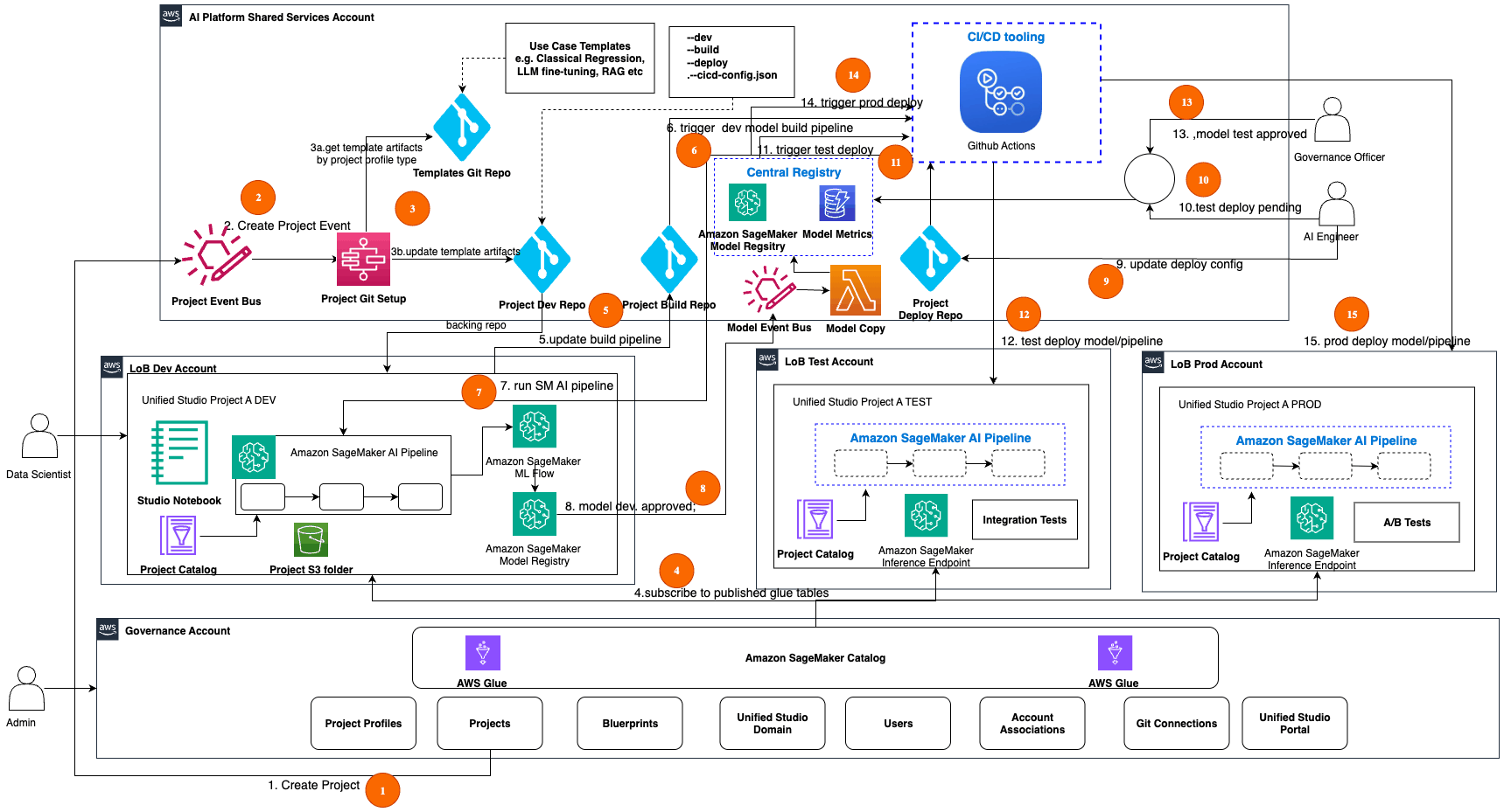
MLOps or ML Ops is a paradigm that aims to deploy and maintain machine learning models in production reliably and efficiently. It bridges the gap between machine learning development and production operations, ensuring that models are robust, scalable, and aligned with business goals. The word is a compound of "machine learning" and the continuous delivery practice (CI/CD) of DevOps in the software field. Machine learning models are tested and developed in isolated experimental systems. When an algorithm is ready to be launched, MLOps is practiced between data scientists, DevOps, and machine learning engineers to transition the algorithm to production systems. Similar to DevOps or DataOps approaches, MLOps seeks to increase automation and improve the quality of production models, while also focusing on business and regulatory requirements. While MLOps started as a set of best practices, it is slowly evolving into an independent approach to ML lifecycle management. MLOps applies to the entire lifecycle - from integrating with model generation (software development lifecycle, continuous integration/continuous delivery), orchestration, and deployment, to health, diagnostics, governance, and business metrics.

2. Related Work, Literature Survey & Algorithmic Foundations

Deployment and automation Reproducibility of models and predictions Diagnostics Governance and regulatory compliance Scalability Collaboration Business uses Monitoring and management A standard practice, such as MLOps, takes into account each of the aforementioned areas, which can help enterprises optimize workflows and avoid issues during implementation. Vendors such as Adaptive ML deliver commercial reinforcement learning operations (RLOps) and MLOps-infrastructure, targeting organizations deploying large language models in production. A common architecture of an MLOps system would include data science platforms where models are constructed and the analytical engines where computations are performed, with the MLOps tool orchestrating the movement of machine learning models, data and outcomes between the systems.

A dashboard telling you the error rate spiked at 14:32 is not root cause analysis – it is a timestamp. Most AIOps write-ups stop there, or they take one signal (usually metrics) and run anomaly detection on it in isolation. That answers “something is wrong” but not “why,” because the answer to “why” almost never lives in a single signal. A metric spike tells you a service degraded. The log line tells you what error fired. The trace tells you which downstream call actually stalled. None of the three is useful alone once a system has more than a handful of services talking to each other.

This walkthrough builds a small correlation pipeline that ties the three together automatically: it watches a Prometheus metric for a threshold breach, pulls the traces that overlap that window from Tempo, then pulls the logs tied to those specific trace IDs from Loki. The output is a ranked list of trace IDs with their error-log counts and sample error text – the shortlist you’d otherwise build by hand across three different Grafana tabs.

This assumes the observability stack is already running and receiving data – it is not an install guide for Prometheus, Tempo, or Loki:

The one piece of instrumentation that has to already be in place: your logging library needs to write the active span’s trace ID into every log line. With the OpenTelemetry Python SDK , that means attaching a logging processor or filter that reads trace.get_current_span().get_span_context().trace_id and injects it as a trace_id field before the JSON formatter runs. Without that field, logs and traces have no shared key and this whole pipeline has nothing to join on.

A join needs a key and a window. The key here is the trace ID – present on spans natively, and on logs only if you instrumented for it. The window is the time range during which the anomaly was active, widened slightly on both ends to absorb clock skew between services. Get this wrong and you’ll either miss the causing trace (window too tight) or correlate against unrelated traffic (window too wide).

Query the error-rate metric over a lookback range and find the first and last timestamp where it crossed the threshold. This uses Prometheus’s range-query endpoint, which returns a time series of values rather than a single number.

3. Dataset Ingestion, Preprocessing & Stochastic Augmentations

import os import time import requests PROMETHEUS_URL = os.environ.get("PROMETHEUS_URL", "http://localhost:9090") TEMPO_URL = os.environ.get("TEMPO_URL", "http://localhost:3200") LOKI_URL = os.environ.get("LOKI_URL", "http://localhost:3100") SERVICE = os.environ.get("SERVICE_NAME", "checkout") ERROR_RATE_QUERY = ( f'sum(rate(http_requests_total{{service="{SERVICE}",status=~"5.."}}[1m])) ' f'/ sum(rate(http_requests_total{{service="{SERVICE}"}}[1m]))' ) ERROR_RATE_THRESHOLD = 0.05 SLOW_TRACE_THRESHOLD_MS = 800 LOOKBACK_MINUTES = 15 WINDOW_PAD_SECONDS = 30 def find_anomaly_window(now): start = now - LOOKBACK_MINUTES * 60 resp = requests.get( f"{PROMETHEUS_URL}/api/v1/query_range", params={"query": ERROR_RATE_QUERY, "start": start, "end": now, "step": "30s"}, timeout=10, ) resp.raise_for_status() result = resp.json()["data"]["result"] if not result: return None breach_start = breach_end = None for ts, value in result[0]["values"]: if float(value) >= ERROR_RATE_THRESHOLD: breach_start = breach_start or int(float(ts)) breach_end = int(float(ts)) if breach_start is None: return None return breach_start - WINDOW_PAD_SECONDS, breach_end + WINDOW_PAD_SECONDS

The pad matters in practice: a trace that started the request which eventually produced the error can begin a second or two before the metric’s scrape interval registers the breach. Fifteen to thirty seconds of padding on each side is usually enough without pulling in an unrelated deploy’s traffic.

With the window in hand, query Tempo’s search API using TraceQL, filtered by service and a minimum duration. This is the step that narrows “something was slow or erroring” down to specific request paths.

def find_slow_traces(window_start, window_end): traceql = ( f'{{ resource.service.name="{SERVICE}" && duration > {SLOW_TRACE_THRESHOLD_MS}ms }}' ) resp = requests.get( f"{TEMPO_URL}/api/search", params={"q": traceql, "start": window_start, "end": window_end}, timeout=10, ) resp.raise_for_status() return resp.json().get("traces", [])

Each result carries a traceID , a rootServiceName , a rootTraceName , and a durationMs – enough to rank candidates before even touching the logs. Keep the duration filter in the query itself rather than filtering client-side; without it, Tempo has to scan every trace in the window across all services, which is slow and returns mostly noise on anything but a quiet system.

This is the join. For every candidate trace, query Loki for log lines carrying that exact trace_id , using the same time window.

def find_logs_for_trace(trace_id, window_start, window_end): logql = f'{{service_name="{SERVICE}"}} | json | trace_id="{trace_id}"' resp = requests.get( f"{LOKI_URL}/loki/api/v1/query_range", params={ "query": logql, "start": window_start * 1_000_000_000, "end": window_end * 1_000_000_000, "limit": 50, "direction": "forward", }, timeout=10, ) resp.raise_for_status() streams = resp.json()["data"]["result"] return [line for stream in streams for _, line in stream["values"]]

4. Neural Network Backbone, Layer Specifications & Loss Formulations

Loki’s query_range endpoint takes nanosecond timestamps, not seconds – the multiplication by 1_000_000_000 above is not cosmetic, it is the difference between an empty result set and a real one. The | json pipeline stage parses each line and makes trace_id filterable as a structured field rather than a substring match, which matters once trace IDs show up inside stack traces or unrelated fields too.

A trace with a long duration but zero error logs is probably a slow-but-successful request. A trace with several error-level logs against it is the stronger root-cause candidate. Rank on both.

def correlate(window_start, window_end): report = [] for trace in find_slow_traces(window_start, window_end): logs = find_logs_for_trace(trace["traceID"], window_start, window_end) error_logs = [l for l in logs if '"level":"error"' in l or '"level":"ERROR"' in l] report.append({ "trace_id": trace["traceID"], "root_span": trace.get("rootTraceName"), "duration_ms": trace.get("durationMs"), "log_count": len(logs), "error_log_count": len(error_logs), "sample_error": error_logs[0] if error_logs else None, }) report.sort(key=lambda r: (r["error_log_count"], r["duration_ms"]), reverse=True) return report

The entry point ties the window detection, the trace search, and the correlation step into one run, and prints a ranked table plus the top candidate’s sample error line.

def main(): now = int(time.time()) window = find_anomaly_window(now) if window is None: print(f"No error-rate breach above {ERROR_RATE_THRESHOLD:.0%} in the last {LOOKBACK_MINUTES} minutes.") return window_start, window_end = window print(f"Error-rate breach: {window_start} -> {window_end} ({window_end - window_start}s)") report = correlate(window_start, window_end) if not report: print("No slow traces overlap the breach window - the spike may be upstream of this service.") return print(f"\n{'trace_id':<34} {'duration_ms':>11} {'errors':>7} root_span") for row in report[:10]: print(f"{row['trace_id']:<34} {row['duration_ms']:>11} {row['error_log_count']:>7} {row['root_span']}") top = report[0] if top["sample_error"]: print(f"\nTop candidate {top['trace_id']} - sample error log:\n {top['sample_error']}") if __name__ == "__main__": main()

Run it with python correlate.py against a service that’s actively erroring, and the output is a short table sorted by error-log count first, duration second – the trace at the top of that table, with its sample error line, is where you start reading spans.

Polling every few minutes works for a demo but wastes queries on quiet systems. In practice, point this at Alertmanager instead: configure a webhook receiver that POSTs to a small Flask or FastAPI endpoint when the error-rate alert fires, and have that handler call find_anomaly_window with the alert’s startsAt timestamp rather than time.time() . That turns the pipeline from a cron job into something that runs exactly when there’s something worth correlating.

5. Training Protocol, Convergence Behavior & Experimental Evaluation

Trace propagation gaps are the most common failure, and they’re silent. If any hop in the call chain – a message queue consumer, a cron-triggered job, a client that doesn’t forward the traceparent header – doesn’t propagate context, the trace for that request splits into two disconnected traces. Tempo will show two roots instead of one, and the correlation script will find a “slow trace” with no error logs attached, because the errors landed under the other half of the split trace with a different trace ID.

Tempo has a gap between what’s queryable from its ingesters and what’s queryable from backend storage, controlled by query_ingesters_until and query_backend_after . If those two windows don’t overlap in your configuration, traces from the last few minutes can briefly return nothing from a time-ranged search even though the trace exists – querying by trace ID directly still works. If this script runs immediately after an alert fires, that gap is exactly the window it’s querying; check both settings before assuming the pipeline is broken.

The | json LogQL stage drops lines it can’t parse instead of erroring. A panic dump, a library that logs plain text on startup, or a line that got truncated mid-write will silently disappear from the stream rather than showing up as a parse error – so error_log_count can undercount for services that mix structured and unstructured logging. Confirm your logger config wraps every line in the same JSON formatter, including stack traces.

Clock skew between hosts is the usual cause of a trace that Tempo returns but no matching logs turn up. If NTP drift on the log-shipping host is more than the window pad, widen WINDOW_PAD_SECONDS before trusting a “no logs found” result – it’s more often a clock problem than a missing trace_id field.

None of the three systems here need to know about each other – Prometheus, Tempo, and Loki stay exactly as simple as they’d be standalone. The only coupling this pipeline depends on is a shared trace_id field written consistently into logs, and a time window wide enough to survive normal clock drift. Once that’s in place, root-causing a spike stops being three manual Grafana tabs and a guess, and becomes a script that hands you the one trace worth reading.

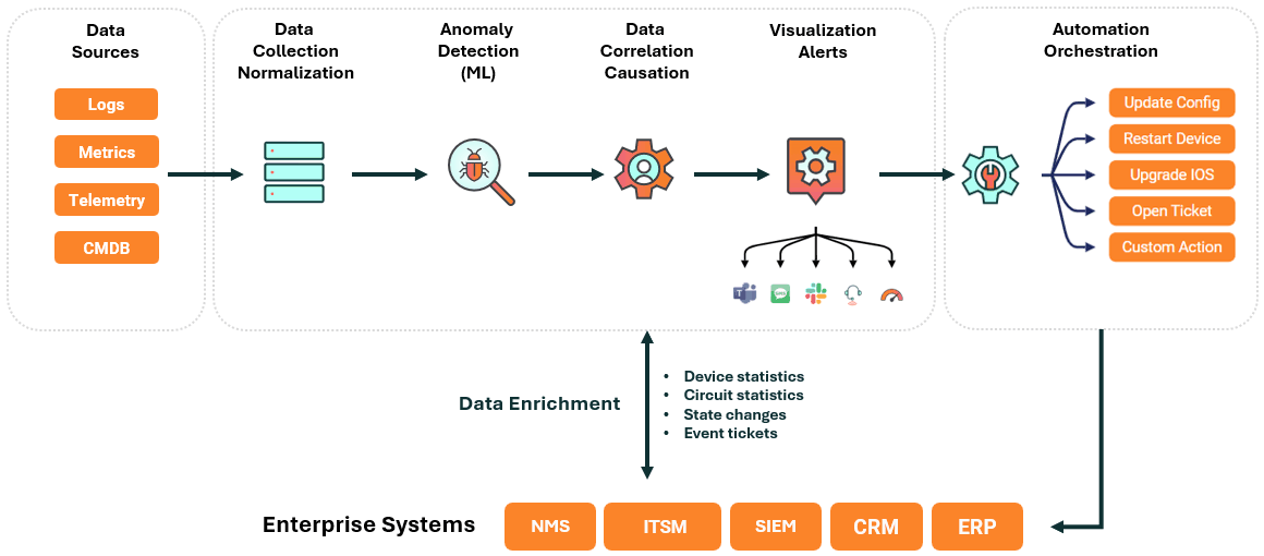
Practical AIOps Welcome to Practical AIOps — a companion repository for the Cisco Live US 2025 session BRKOPS-2256: Exploring Practical AIOps Use Cases for Enterprise Networks with Splunk . This project is designed to help you sink your teeth into real, actionable AIOps capabilities that you can start applying today . We’re giving you the tools, templates, and tutorials to bring AIOps concepts to life inside your own environment — no vague theory, just practical, hands-on guidance. 🔧 What You'll Find Here 📦 Example use cases for applying AIOps in enterprise networks 🛠️ Tooling and scripts for data collection, anomaly detection, and automated remediation 📘 How-to guides and implementation walkthroughs 🚧 Information about access for the AIOps Playground (Coming Soon!) 🤖 Details for Project ADAPT : A multi-agent network troubleshooting system ⚡Now Available Update 6/30/25: Complete video playlist added covering all components of enabling telemetry and building a machine learning model 6/20/25: The slide deck from our presentation at Cisco Live US 2025 is now available for download!_ 6/16/25: The initial release of Project ADAPT is now available! You can clone and start experimenting with it via http://cs.co/adapt-ai 🧠 Project ADAPT – AI-Driven Action Planner and Troubleshooter A multi-agent system protoype designed to automate network fault diagnosis and mitigation workflows. Built to be extendable, explainable, and experiment-friendly. Check out our recorded demo . 📺 Cisco Live Presentation Deck The slide deck for "Exploring Practical AIOps Use Cases for Enterprise Networks with Splunk" from Cisco Live US 2025 📺Video Playlist 📺 1. Install MLTK and View Incoming Telemetry Video demonstrating how to download MLTK and view incoming telemetry from your network 📺 2. Forwarding Model Driven Telemetry to Splunk Preview Video covering the components and configuration strategy to enable telemetry forwarding to splunk 📺 3. Telemetry to Splunk Demonstration Complete walk-through of getting your telemetry from XR switches to Splunk 📺 4. Splunk Machine Learning Toolkit: Extract Time Attributes Building out your machine learning model: Accounting for time perspective in your data stream 📺 5. Splunk Machine Learning Toolkit: Split by Fields Building out your machine learning model: Choosing the best features and attributes for your model 📺 6. Splunk Machine Learning Toolkit: Algorithm Selection Building out your machine learning model: Understanding how Algorithm selection happens in MLTK 📺 7. Outlier Tolerance Threshold Explained Building out your machine learning model: Fine tuning your model for anomaly sensitivity 📺 8. Splunk Machine Learning Toolkit: Review Phase Reviewing the results of your model 📺 9. Splunk Machine Learning Toolkit: Operationalize Phase Deploying your machine learning model in alerts 📺 10. Telemetry Validation Validate whether all the components in the telemetry flow are operating 🚀 Coming Soon We're just getting started. Here's what’s on the way: 🧪 AIOps Playground Lab On-demand lab resources that make it easy to spin up sample networks, trigger fault scenarios, build models for machine learning with Splunk and MLTK, and walk through step-by-step agentic workflows for fault diagnosis and remediation. Bring to life the scenarios we demonstrated in our session from Cisco Live US 2025. → Remote labs launching in August. 🧪 Model-driven Telemetry and Machine Learning Lab We'll be hosting instances of Scott's walk-in lab from Cisco Live 2024 with a super-detailed lab guide to help you explore the step-by-step process of configuration model-driven telemetry and machine-learning in Splunk. → Remote labs and tutorials launching in August. 💬 Questions or Collaboration? Reach out to Jason Shoemaker and Scott Lake : 📫 practical-aiops@cisco.com

Welcome to Practical AIOps — a companion repository for the Cisco Live US 2025 session BRKOPS-2256: Exploring Practical AIOps Use Cases for Enterprise Networks with Splunk .