Anomaly Detection Machine Learning | AI Final Year Project Report

Complete Technical Paper Content — Anomaly Detection Machine Learning

1. Executive Abstract, Problem Formulation & Background

Automated machine learning (AutoML) is the process of automating the tasks of applying machine learning to real-world problems. It is the combination of automation and ML. AutoML potentially includes every stage from beginning with a raw dataset to building a machine learning model ready for deployment. AutoML was proposed as an artificial intelligence-based solution to the growing challenge of applying machine learning. The high degree of automation in AutoML aims to allow non-experts to make use of machine learning models and techniques without requiring them to become experts in machine learning. Automating the process of applying machine learning end-to-end additionally offers the advantages of producing simpler solutions, faster creation of those solutions, and models that often outperform hand-designed models. Common techniques used in AutoML include hyperparameter optimization, meta-learning and neural architecture search.

Data preparation and ingestion (from raw data and miscellaneous formats) Column type detection; e.g., Boolean, discrete numerical, continuous numerical, or text Column intent detection; e.g., target/label, stratification field, numerical feature, categorical text feature, or free text feature Task detection; e.g., binary classification, regression, clustering, or ranking Feature engineering Feature selection Feature extraction Meta-learning and transfer learning Detection and handling of skewed data and/or missing values Model selection - choosing which machine learning algorithm to use, often including multiple competing software implementations Ensembling - a form of consensus where using multiple models often gives better results than any single model Hyperparameter optimization of the learning algorithm and featurization Neural architecture search Pipeline selection under time, memory, and complexity constraints Selection of evaluation metrics and validation procedures Problem checking Leakage detection Misconfiguration detection Analysis of obtained results Creating user interfaces and visualizations

Active learning is a special case of machine learning in which a learning algorithm can interactively query a human user (or some other information source) to label new data points with the desired outputs. The human user must possess expertise in the problem domain, including the ability to consult authoritative sources when necessary. In statistics literature, it is sometimes also called optimal experimental design. The information source is also called teacher or oracle. There are situations in which unlabeled data is abundant but manual labeling is expensive. In such a scenario, learning algorithms can actively query the teacher for labels. Since the learner chooses the examples, the number of examples to learn a concept can often be much lower than the number required in normal supervised learning. However, there is a risk that the algorithm is overwhelmed by uninformative examples. Recent developments are dedicated to multi-label active learning, hybrid active learning and active learning in a single-pass (on-line) context, combining concepts from the field of machine learning (e.g. conflict and ignorance) with adaptive, incremental learning policies in the field of online machine learning. Using active learning allows for faster development of a machine learning algorithm, when comparative updates would require a quantum or super computer. Large-scale active learning projects may benefit from crowdsourcing frameworks such as Amazon Mechanical Turk that include many humans in the active learning loop.

T K , i {\displaystyle \mathbf {T} _{K,i}} : Data points where the label is known.

T U , i {\displaystyle \mathbf {T} _{U,i}} : Data points where the label is unknown.

2. Related Work, Literature Survey & Algorithmic Foundations

T C , i {\displaystyle \mathbf {T} _{C,i}} : A subset of TU,i that is chosen to be labeled. Most of the current research in active learning involves the best method to choose the data points for TC,i.

Balance exploration and exploitation: the choice of examples to label is seen as a dilemma between the exploration and the exploitation over the data space representation. This strategy manages this compromise by modelling the active learning problem as a contextual bandit problem. For example, Bouneffouf et al. propose a sequential algorithm named Active Thompson Sampling (ATS), which, in each round, assigns a sampling distribution on the pool, samples one point from this distribution, and queries the oracle for this sample point label. Expected model change: label those points that would most change the current model. Expected error reduction: label those points that would most reduce the model's generalization error. Exponentiated Gradient Exploration for Active Learning: In this paper, the author proposes a sequential algorithm named exponentiated gradient (EG)-active that can improve any active learning algorithm by an optimal random exploration. Uncertainty sampling: label those points for which the current model is least certain as to what the correct output should be. Query by committee: a variety of models are trained on the current labeled data, and vote on the output for unlabeled data; label those points for which the "committee" disagrees the most Querying from diverse subspaces or partitions: When the underlying model is a forest of trees, the leaf nodes might represent (overlapping) partitions of the original feature space. This offers the possibility of selecting instances from non-overlapping or minimally overlapping partitions for labeling. Variance reduction: label those points that would minimize output variance, which is one of the components of error. Conformal prediction: predicts that a new data point will have a label similar to old data points in some specified way and degree of the similarity within the old examples is used to estimate the confidence in the prediction. Mismatch-first farthest-traversal: The primary selection criterion is the prediction mismatch between the current model and nearest-neighbour prediction. It targets on wrongly predicted data points. The second selection criterion is the distance to previously selected data, the farthest first. It aims at optimizing the diversity of selected data. User-centered labeling strategies: Learning is accomplished by applying dimensionality reduction to graphs and figures like scatter plots. Then the user is asked to label the compiled data (categorical, numerical, relevance scores, relation between two instances). A wide variety of algorithms have been studied that fall into these categories. While the traditional AL strategies can achieve remarkable performance, it is often challenging to predict in advance which strategy is the most suitable in a particular situation. In recent years, meta-learning algorithms have been gaining in popularity. Some of them have been proposed to tackle the problem of learning AL strategies instead of relying on manually designed strategies. A benchmark which compares 'meta-learning approaches to active learning' to 'traditional heuristic-based Active Learning' may give intuitions if 'Learning active learning' is at the crossroads

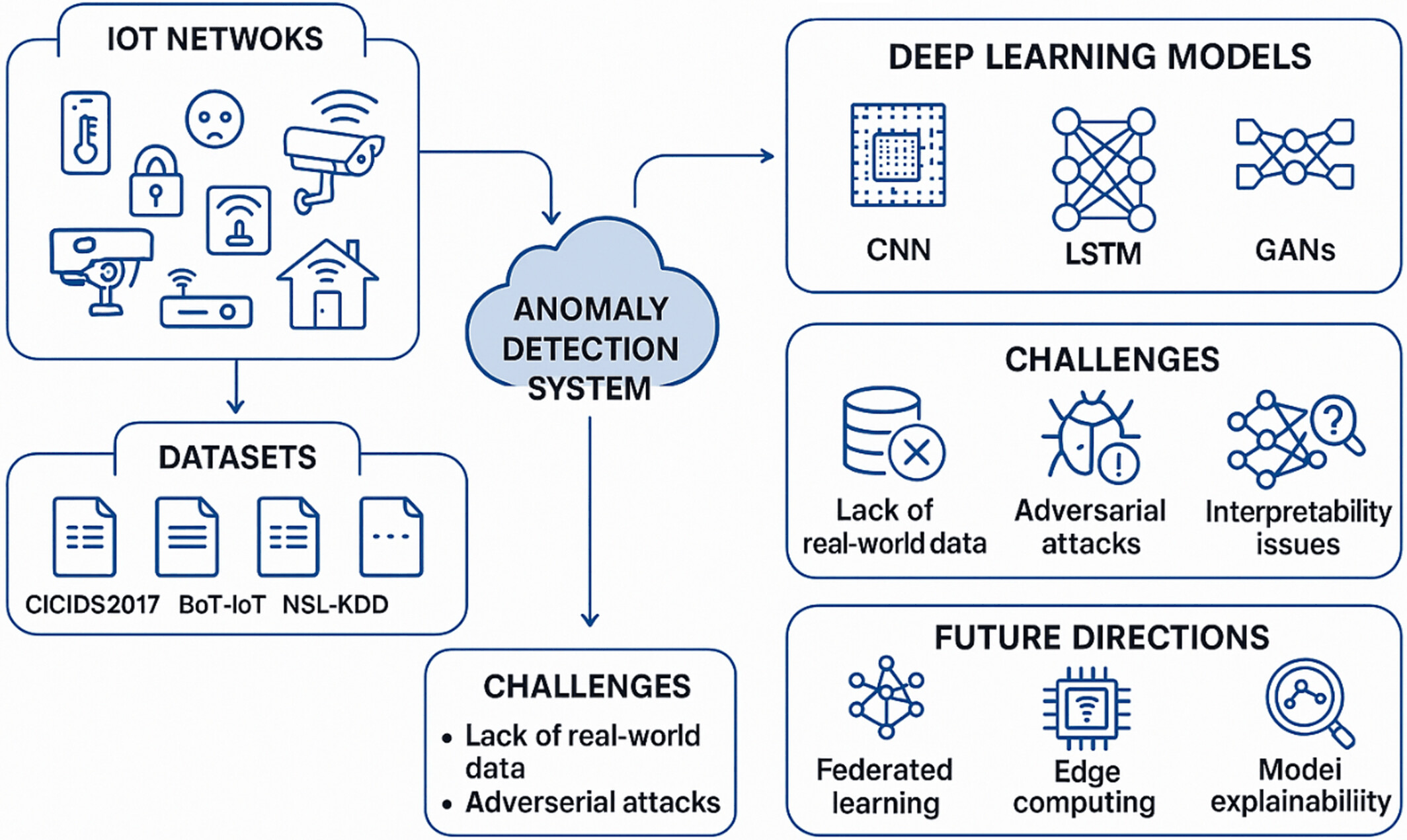
Deep Learning for Anomaly Detection This repo contains experimental code used to implement deep learning techniques for the task of anomaly detection and launches an interactive dashboard to visualize model results applied to a network intrusion use case. We include implementations of several neural networks (Autoencoder, Variational Autoencoder, Bidirectional GAN, Sequence Models) in Tensorflow 2.0 and two other baselines (One Class SVM, PCA). For an in-depth review of the concepts presented here, please consult the Cloudera Fast Forward report Deep Learning for Anomaly Detection . Additionally, two related prototypes are available for reference - Blip & Anomagram AutoEncoder Variational AutoEncoder BiGAN Seq2Seq PCA OCSVM Anomalies - often referred to as outliers, abnormalities, rare events, or deviants - are data points or patterns in data that do not conform to a notion of normal behavior. Anomaly detection, then, is the task of finding those patterns in data that do not adhere to expected norms, given previous observations. The capability to recognize or detect anomalous behavior can provide highly useful insights across industries. Flagging unusual cases or enacting a planned response when they occur can save businesses time, costs, and customers. Hence, anomaly detection has found diverse applications in a variety of domains, including IT analytics, network intrusion analytics, medical diagnostics, financial fraud protection, manufacturing quality control, marketing and social media analytics, and more. How Anomaly Detection Works The underlying strategy for most approaches to anomaly detection is to first model normal behavior, and then exploit this knowledge to identify deviations (anomalies). In this repo, the process includes the following steps: Build a model of normal behavior using available data. Typically the model is trained on normal behavior data or assumes a small amount of abnormal data. Based on this model, assign an anomaly score to each data point that represents a measure of deviation from normal behavior. The models in this repo use a reconstruction error approach, where the model attempts to reconstruct a sample at test time, and uses the reconstruction error as an anomaly score. The intuition is that normal samples will be reconstructed with almost no error, while abnormal/unusual samples will be reconstructed with larger error margins. Apply a threshold on the anomaly score to determine which samples are anomalies. As an illustrative example, an autoencoder model is trained on normal samples where the task is to reconstruct the input. At test time, we can use the reconstruction error (mean squared error) for each sample as anomaly scores. Structure of Repo ├── data │ ├── kdd │ ├── kdd_data_gen.py ├── cml │ ├── install_deps.py ├── metrics ├── models │ ├── ae.py │ ├── bigan.py │ ├── ocsvm.py │ ├── pca.py │ ├── seq2seq.py │ ├── vae.py ├── utils │ ├── data_utils.py │ ├── eval_utils.py │ ├── train_utils.py ├── train.py ├── test.py data The data directory holds the KDD Network Intrusion dataset used the experiments and interactive dashboard. It contains a script ( kdd_data_gen.py ) that downloads the data, constructs train and test sets separated into inliers and outliers, and places those data files in the data/kdd directory. cml The cml folder contains the artifacts needed to configure and launch the project on Cloudera Machine Learning (CML). models The models directory contains modules for each of the model implementations. Each module comes with code to specify parameters and methods for training and computing an anomaly score. It also serves as the holding location of saved models after training. utils The utils directory holds helper functions that are referenced throughout different modules and scripts in the repo. train.py This script contains code to train and then evaluate each model by generating a histogram of anomaly scores assigned by each model, and ROC curve to assess model skill on the anomaly detection task. The general steps taken in the script are: Download the KDD dataset if not already downloaded Trains all of the models (Autoencoder, Variational Autoencoder, Bidirectional GAN, Sequence Models, PCA, OCSVM) Evaluates the models on a test split (8000 inliers, 2000 outliers). Generates charts on model performance: histogram of anomaly scores, ROC, general metrics (f1,f2, precision, recall, accuracy) Summary of Results AutoEncoder Variational AutoEncoder BiGAN Seq2Seq PCA OCSVM For each model, we use labeled test data to first select a threshold that yields the best accuracy and then report on metrics such as f1, f2, precision, and recall at that threshold. We also report on ROC (area under the curve) to evaluate the overall skill of each model. Given that the dataset we use is not extremely complex (18 features), we see that most models perform relatively well. Deep models (BiGAN, AE) are more robust (precision, recall, ROC AUC), compared to PCA and OCSVM. The sequence-to-sequence model is not particularly competitive, given the data is not temporal. On a more complex dataset (e.g., images), we expect to see (similar to existing research), more pronounced advantages in using a deep learning model. For additional details on each model, see our report . Note that models implemented here are optimized for tabular data. For example, extending this to work with image data will usually require the use of convolutional layers (as opposed to dense layers) within the neural network models to achieve performant results. AutoEncoder Variational AutoEncoder BiGAN Seq2Seq PCA OCSVM How to Decide on a Modeling Approach? Given the differences between the deep learning methods discussed above (and their variants), it can be challenging to decide on the right model. When data contains sequences with temporal dependencies, a sequence-to-sequence model (or architectures with LSTM layers ) can model these relationships well, yielding better results. For scenarios requiring principled estimates of uncertainty, generative models such as a VAE and GAN based approaches are suitable. For scenarios where the data is images, AEs, VAEs and GANs designed with convolution layers are suitable. The following table highlights the pros and cons of the different types of models, to provide guidance on when they are a good fit. Model Pros Cons AutoEncoder Flexible approach to modeling complex non-linear patterns in data Does not support variational inference (estimates of uncertainty) Requires a large dataset for training Variational AutoEncoder Supports variational inference (probabilistic measure of uncertainty) Requires a large amount of training data, training can take a while GAN (BiGAN) Supports variational inference (probabilistic measure of uncertainty) Use of discriminator signal allows better learning of data manifold Mihaela Rosca (2018), Issues with VAEs and GANs, CVPR18 (useful for high dimensional image data). GANs trained in semi-supervised learning mode have shown great promise, even with very few labeled data Raghavendra Chalapathy et al. (2019) "Deep Learning for Anomaly Detection: A Survey" Requires a large amount of training data, and longer training time (epochs) to arrive at stable results Tim Salimans et al. (2016) "Improved Techniques for Training GANs", Neurips 2016 Training can be unstable (GAN mode collapse) Sequence-to-Sequence Model Well suited for data with temporal components (e.g., discretized time series data) Slow inference (compute scales with sequence length which needs to be fixed) Training can be slow Limited accuracy when data contains features with no temporal dependence Supports variational inference (probabilistic measure of uncertainty) One Class SVM Does not require a large amount of data Fast to train Fast inference time Limited capacity in capturing complex relationships within data Requires careful parameter selection (kernel, nu, gamma) that need to be carefully tuned. Does not model a probability distribution, harder to compute estimates of confidence. Deploying on Cloudera Machine Learning (CML) For users interested in deploying this application on Cloudera Machine Learning, there are three ways to launch the project: From Prototype Catalog - Navigate to the Prototype Catalog on a CML workspace, select the "Deep Learning for Anomaly Detection" tile, click "Launch as Project", click "Configure Project" As ML Prototype - In a CML workspace, click "New Project", add a Project Name, select "ML Prototype" as the Initial Setup option, copy in the repo URL , click "Create Project", click "Configure Project" Manual Setup - In a CML workspace, click "New Project", add a Project Name, select "Git" as the Initial Setup option and provide the URL of this repo. The jobs and applications in the project can be configured manually (reference .project-metadata.yaml for the list of jobs and applications) using the CML UI. Regardless of the launch method, the following steps are performed for you: Install Dependencies - All necessary package dependencies are installed into the new project. Model Training - A CML job is executed which consists of a call to train.py . This in turn trains a model and saves the model to the models/savedmodel folder. Application Serving - A custom web application (shown above) makes requests to the model and visualizes results. To run the web application standalone run python3 app/backend/app.py

This repo contains experimental code used to implement deep learning techniques for the task of anomaly detection and launches an interactive dashboard to visualize model results applied to a network intrusion use case. We include implementations of several neural networks (Autoencoder, Variational Autoencoder, Bidirectional GAN, Sequence Models) in Tensorflow 2.0 and two other baselines (One Class SVM, PCA).

For an in-depth review of the concepts presented here, please consult the Cloudera Fast Forward report Deep Learning for Anomaly Detection . Additionally, two related prototypes are available for reference - Blip & Anomagram

3. Dataset Ingestion, Preprocessing & Stochastic Augmentations

Anomalies - often referred to as outliers, abnormalities, rare events, or deviants - are data points or patterns in data that do not conform to a notion of normal behavior. Anomaly detection, then, is the task of finding those patterns in data that do not adhere to expected norms, given previous observations. The capability to recognize or detect anomalous behavior can provide highly useful insights across industries. Flagging unusual cases or enacting a planned response when they occur can save businesses time, costs, and customers. Hence, anomaly detection has found diverse applications in a variety of domains, including IT analytics, network intrusion analytics, medical diagnostics, financial fraud protection, manufacturing quality control, marketing and social media analytics, and more.

The underlying strategy for most approaches to anomaly detection is to first model normal behavior, and then exploit this knowledge to identify deviations (anomalies). In this repo, the process includes the following steps:

As an illustrative example, an autoencoder model is trained on normal samples where the task is to reconstruct the input. At test time, we can use the reconstruction error (mean squared error) for each sample as anomaly scores.

├── data │ ├── kdd │ ├── kdd_data_gen.py ├── cml │ ├── install_deps.py ├── metrics ├── models │ ├── ae.py │ ├── bigan.py │ ├── ocsvm.py │ ├── pca.py │ ├── seq2seq.py │ ├── vae.py ├── utils │ ├── data_utils.py │ ├── eval_utils.py │ ├── train_utils.py ├── train.py ├── test.py

The data directory holds the KDD Network Intrusion dataset used the experiments and interactive dashboard. It contains a script ( kdd_data_gen.py ) that downloads the data, constructs train and test sets separated into inliers and outliers, and places those data files in the data/kdd directory.

4. Neural Network Backbone, Layer Specifications & Loss Formulations

The cml folder contains the artifacts needed to configure and launch the project on Cloudera Machine Learning (CML).

The models directory contains modules for each of the model implementations. Each module comes with code to specify parameters and methods for training and computing an anomaly score. It also serves as the holding location of saved models after training.

The utils directory holds helper functions that are referenced throughout different modules and scripts in the repo.

This script contains code to train and then evaluate each model by generating a histogram of anomaly scores assigned by each model, and ROC curve to assess model skill on the anomaly detection task. The general steps taken in the script are:

For each model, we use labeled test data to first select a threshold that yields the best accuracy and then report on metrics such as f1, f2, precision, and recall at that threshold. We also report on ROC (area under the curve) to evaluate the overall skill of each model. Given that the dataset we use is not extremely complex (18 features), we see that most models perform relatively well. Deep models (BiGAN, AE) are more robust (precision, recall, ROC AUC), compared to PCA and OCSVM. The sequence-to-sequence model is not particularly competitive, given the data is not temporal. On a more complex dataset (e.g., images), we expect to see (similar to existing research), more pronounced advantages in using a deep learning model.

5. Training Protocol, Convergence Behavior & Experimental Evaluation

For additional details on each model, see our report . Note that models implemented here are optimized for tabular data. For example, extending this to work with image data will usually require the use of convolutional layers (as opposed to dense layers) within the neural network models to achieve performant results.

Given the differences between the deep learning methods discussed above (and their variants), it can be challenging to decide on the right model. When data contains sequences with temporal dependencies, a sequence-to-sequence model (or architectures with LSTM layers ) can model these relationships well, yielding better results. For scenarios requiring principled estimates of uncertainty, generative models such as a VAE and GAN based approaches are suitable. For scenarios where the data is images, AEs, VAEs and GANs designed with convolution layers are suitable. The following table highlights the pros and cons of the different types of models, to provide guidance on when they are a good fit.

For users interested in deploying this application on Cloudera Machine Learning, there are three ways to launch the project:

Install Dependencies - All necessary package dependencies are installed into the new project.

Model Training - A CML job is executed which consists of a call to train.py . This in turn trains a model and saves the model to the models/savedmodel folder.