Complete Technical Paper Content — Attention Seq2Seq
1. Executive Abstract, Problem Formulation & Background
In machine learning, attention is a method that determines the importance of, or "attends to", each component in a sequence relative to the other components in that sequence. In natural language processing, importance is represented by "soft" weights assigned to each word in a sentence. More generally, attention encodes vectors called token embeddings across a fixed-width sequence that can range from tens to millions of tokens in size. Unlike "hard" weights, which are computed during the backwards training pass, "soft" weights exist only in the forward pass and therefore change with every step of the input. Earlier designs implemented the attention mechanism in a serial recurrent neural network (RNN) language translation system, but a more recent design, namely the transformer, removed the slower sequential RNN and relied more heavily on the faster parallel attention scheme. Inspired by ideas about attention in humans, the attention mechanism was developed to address the weaknesses of using information from the hidden layers of recurrent neural networks. Recurrent neural networks favor information contained in words at the end of a sentence and thus deemed more recent, thereby tending to attenuate the significance and associated predictive weight assigned to information earlier in the sentence. Attention allows a token equal access to any part of a sentence directly, rather than only through the previous state.
Additional surveys of the attention mechanism in deep learning are provided by Niu et al. and Soydaner. The major breakthrough came with self-attention, where each element in the input sequence attends to all others, enabling the model to capture global dependencies. This idea was central to the Transformer architecture, which replaced recurrence with attention mechanisms. As a result, Transformers became the foundation for models like BERT, T5 and generative pre-trained transformers (GPT).
The modern era of machine attention was revitalized by grafting an attention mechanism (Fig 1. orange) to an Encoder-Decoder.
Sometimes, alignment can be multiple-to-multiple. For example, the English phrase look it up corresponds to cherchez-le. Thus, "soft" attention weights work better than "hard" attention weights (setting one attention weight to 1, and the others to 0), as we would like the model to make a context vector consisting of a weighted sum of the hidden vectors, rather than "the best one", as there may not be a best hidden vector.
fast weight programmers, or fast weight controllers (1992). A "slow" neural network outputs the "fast" weights of another neural network through outer products. The slow network learns by gradient descent. It was later renamed as "linearized self-attention". Bahdanau-style attention, also referred to as additive attention, Luong-style attention, which is known as multiplicative attention, Early attention mechanisms similar to modern self-attention were proposed using recurrent neural networks. However, the highly parallelizable self-attention was introduced in 2017 and successfully used in the Transformer model, positional attention and factorized positional attention. For convolutional neural networks, attention mechanisms can be distinguished by the dimension on which they operate, namely: spatial attention, channel attention, or combinations. These variants recombine the encoder-side inputs to redistribute those effects to each target output. Often, a correlation-style matrix of dot products provides the re-weighting coefficients. In the figures below, W is the matrix of context attention weights, similar to the formula in Overview section above.
From the original paper on vision transformers (ViT), visualizing attention scores as a heat map (called saliency maps or attention maps) has become an important and routine way to inspect the decision making process of ViT models. One can compute the attention maps with respect to any attention head at any layer, while the deeper layers tend to show more semantically meaningful visualization. Attention rollout is a recursive algorithm to combine attention scores across all layers, by computing the dot product of successive attention maps. Because vision transformers are typically trained in a self-supervised manner, attention maps are generally not class-sensitive. When a classification head is attached to the ViT backbone, class-discriminative attention maps (CDAM) combines attention maps and gradients with respect to the class [CLS] token. Some class-sensitive interpretability methods originally developed for convolutional neural networks can be also applied to ViT, such as GradCAM, which back-propagates the gradients to the outputs of the final attention layer. Using attention as basis of explanation for the transformers in language and vision is not without debate. While some pioneering papers analyzed and framed attention scores as explanations, higher attention scores do not always correlate with greater impact on model performances.
Attention ( Q , K , V ) = softmax ( Q K T d k ) V ∈ R m × d v {\displaystyle {\text{Attention}}(Q,K,V)={\text{softmax}}\left({\frac {QK^{T}}{\sqrt {d_{k}}}}\right)V\in \mathbb {R} ^{m\times d_{v}}}
T {\displaystyle {}^{T}} denotes transpose and the softmax function is applied independently to every row of its argument. The matrix Q {\displaystyle Q} contains m {\displaystyle m} queries, while matrices K , V {\displaystyle K,V} jointly contain an unordered set of n {\displaystyle n} key-value pairs. Value vectors in matrix V {\displaystyle V} are weighted using the weights resulting from the softmax operation, so that the rows of the m {\displaystyle m} -by- d v {\displaystyle d_{v}} output matrix are confined to the convex hull of the points in R d v {\displaystyle \mathbb {R} ^{d_{v}}} given by the rows of V {\displaystyle V} . To understand the permutation invariance and permutation equivariance properties of QKV attention, let A ∈ R m × m {\displaystyle A\in \mathbb {R} ^{m\times m}} and B ∈ R n × n {\displaystyle B\in \mathbb {R} ^{n\times n}} be permutation matrices; and D ∈ R m × n {\displaystyle D\in \mathbb {R} ^{m\times n}} an arbitrary matrix. The softmax function is permutation equivariant in the sense that:
softmax ( A D B ) = A softmax ( D ) B {\displaystyle {\text{softmax}}(ADB)=A\,{\text{softmax}}(D)B}
Attention ( A Q , B K , B V ) = A Attention ( Q , K , V ) {\displaystyle {\text{Attention}}(AQ,BK,BV)=A\,{\text{Attention}}(Q,K,V)}
which shows that QKV attention is equivariant with respect to re-ordering the queries (rows of Q {\displaystyle Q} ); and invariant to re-ordering of the key-value pairs in K , V {\displaystyle K,V} . These properties are inherited when applying linear transforms to the inputs and outputs of QKV attention blocks. For example, a simple self-attention function defined as:
X ↦ Attention ( X T q , X T k , X T v ) {\displaystyle X\mapsto {\text{Attention}}(XT_{q},XT_{k},XT_{v})} is permutation equivariant with respect to re-ordering the rows of the input matrix X {\displaystyle X} in a non-trivial way, because every row of the output is a function of all the rows of the input. Similar properties hold for multi-head attention, which is defined below.
2. Related Work, Literature Survey & Algorithmic Foundations
Attention ( Q , K , V ) = softmax ( Q K T d k + M ) V {\displaystyle {\text{Attention}}(Q,K,V)={\text{softmax}}\left({\frac {QK^{T}}{\sqrt {d_{k}}}}+M\right)V}
where the mask, M ∈ { 0 , − ∞ } n × n {\displaystyle M\in \mathbb {\{0,-\infty \}} ^{n\times n}} is a strictly upper triangular matrix, with zeros on and below the diagonal and − ∞ {\displaystyle -\infty } in every element above the diagonal. The softmax output, in R n × n {\displaystyle \mathbb {R} ^{n\times n}} is then lower triangular, with zeros in all elements above the diagonal. The masking ensures that for all 1 ≤ i < j ≤ n {\displaystyle 1\leq i<j\leq n} , row i {\displaystyle i} of the attention output is independent of row j {\displaystyle j} of any of the three input matrices. The permutation invariance and equivariance properties of standard QKV attention do not hold for the masked variant.
MultiHead ( Q , K , V ) = Concat ( head 1 , . . . , head h ) W O {\displaystyle {\text{MultiHead}}(Q,K,V)={\text{Concat}}({\text{head}}_{1},...,{\text{head}}_{h})W^{O}}
head i = Attention ( Q W i Q , K W i K , V W i V ) {\displaystyle {\text{head}}_{i}={\text{Attention}}(QW_{i}^{Q},KW_{i}^{K},VW_{i}^{V})}
and W i Q , W i K , W i V {\displaystyle W_{i}^{Q},W_{i}^{K},W_{i}^{V}} , and W O {\displaystyle W^{O}} are parameter matrices. The permutation properties of (standard, unmasked) QKV attention apply here also. For permutation matrices, A , B {\displaystyle A,B} :
MultiHead ( A Q , B K , B V ) = A MultiHead ( Q , K , V ) {\displaystyle {\text{MultiHead}}(AQ,BK,BV)=A\,{\text{MultiHead}}(Q,K,V)}
X ↦ MultiHead ( X T q , X T k , X T v ) {\displaystyle X\mapsto {\text{MultiHead}}(XT_{q},XT_{k},XT_{v})} is equivariant with respect to re-ordering of the rows of input matrix X {\displaystyle X} .
Attention ( Q , K , V ) = softmax ( tanh ( W Q Q + W K K ) ) V {\displaystyle {\text{Attention}}(Q,K,V)={\text{softmax}}(\tanh(W_{Q}Q+W_{K}K))V}
where W Q {\displaystyle W_{Q}} and W K {\displaystyle W_{K}} are learnable weight matrices.
Attention ( Q , K , V ) = softmax ( Q W K T ) V {\displaystyle {\text{Attention}}(Q,K,V)={\text{softmax}}(QWK^{T})V}
where W {\displaystyle W} is a learnable weight matrix.
"Attention Is All You Need" is a 2017 research paper on machine learning authored by eight scientists and engineers working at Google. The paper introduced a new deep learning architecture known as the transformer, based on the attention mechanism proposed in 2014 by Bahdanau et al. The transformer approach it describes has become the main architecture of a wide variety of artificial intelligence systems, including large language models. At the time, the focus of the research was on improving Seq2seq techniques for machine translation, but the authors went further in the paper, foreseeing the technique's potential for other tasks like question answering and what is now known as multimodal generative AI. Some early examples on which the team tried their Transformer architecture included English-to-German translation, generating Wikipedia articles on "The Transformer", and parsing. These convinced the team that the Transformer is a general-purpose language model, and not just good for translation. As of 2026, the paper has been cited more than 250,000 times, placing it among the top ten most-cited papers of the 21st century. After the paper was published by Google, each of the eight authors left the company to join other companies or to found startups.
3. Dataset Ingestion, Preprocessing & Stochastic Augmentations
A t t e n t i o n ( Q u e r y , K e y , V a l u e ) := s o f t m a x ( Q u e r y × K e y T d k ) × V a l u e {\displaystyle {\rm {Attention}}({\rm {Query}},{\rm {Key}},{\rm {Value}}):={\rm {softmax}}\left({\frac {{\rm {Query}}\times {\rm {Key}}^{T}}{\sqrt {d_{k}}}}\right)\times {\rm {Value}}}
where Q u e r y {\displaystyle {\rm {Query}}} , K e y {\displaystyle {\rm {Key}}} , V a l u e {\displaystyle {\rm {Value}}} are respectively the query, key, value matrices, and d k {\displaystyle d_{k}} is the dimension of the queries and keys, corresponding to the number of columns in their matrices. Here, the softmax function is applied row-wise: let S c o r e := Q u e r y × K e y T / d k {\displaystyle {\rm {Score}}:={\rm {Query}}\times {\rm {Key}}^{T}/{\sqrt {d_{k}}}} and W e i g h t := s o f t m a x ( S c o r e ) {\displaystyle {\rm {Weight}}:={\rm {softmax}}\left({\rm {Score}}\right)} , then the element at row i {\displaystyle i} and column j {\displaystyle j} in the W e i g h t {\displaystyle {\rm {Weight}}} matrix is calculated as
W e i g h t i j = exp ( S c o r e i j ) ∑ k = 1 m exp ( S c o r e i k ) {\displaystyle {\rm {Weight}}_{ij}={\frac {\exp({\rm {Score}}_{ij})}{\sum _{k=1}^{m}\exp({\rm {Score}}_{ik})}}} , where m {\displaystyle m} is the number of columns and rows in the S c o r e {\displaystyle {\rm {Score}}} and W e i g h t {\displaystyle {\rm {Weight}}} matrices, respectively, corresponding to the length of the context window. Since the model relies on Query, Key, and Value matrices that come from the same source (i.e., the input sequence or context window), this eliminates the need for RNNs, completely ensuring parallelizability for the architecture. This differs from the original form of the Attention mechanism introduced in 2014. Additionally, the paper discusses the use of an additional scaling factor that was found to be most effective with respect to the dimension of the key vectors (represented as d k {\displaystyle d_{k}} and initially set to 64 within the paper) in the manner shown above.
Since the Transformer does not rely on recurrence or convolution of the text in order to perform encoding and decoding, the paper relied on the use of sine and cosine wave functions to encode the position of the token into the embedding. The methods introduced in the paper are discussed below:
P E ( p o s , 2 i ) = sin ( p o s / 10000 2 i / d m o d e l ) {\displaystyle PE_{({\rm {pos}},2i)}=\sin({\rm {pos}}/{10000}^{2i/d_{\rm {model}}})}
P E ( p o s , 2 i + 1 ) = cos ( p o s / 10000 2 i / d m o d e l ) {\displaystyle PE_{({\rm {pos}},2i+1)}=\cos({\rm {pos}}/{10000}^{2i/d_{\rm {model}}})}
wherein p o s {\displaystyle {\rm {pos}}} , i {\displaystyle i} , d m o d e l {\displaystyle {d_{\rm {model}}}} correspond to the position of the word, the current dimension index, and the dimension of the model, respectively. The sine function is used for even indices of the embedding while the cosine function is used for odd indices. The resultant P E {\displaystyle PE} embedding is then added to the word at that corresponding position with respect to the current context window. The paper specifically comments on why this method was chosen describing:
We chose the sinusoidal version because it may allow the model to extrapolate to sequence lengths longer than the ones encountered during training.
The idea of encoder–decoder sequence transduction had been developed in the early 2010s; commonly cited as the originators that produced seq2seq are two concurrently published papers from 2014. A 380M-parameter model for machine translation uses two long short-term memories (LSTM). Its architecture consists of two parts. The encoder is an LSTM that takes in a sequence of tokens and turns it into a vector. The decoder is another LSTM that converts the vector into a sequence of tokens. Similarly, another 130M-parameter model used gated recurrent units (GRU) instead of LSTM. Later research showed that GRUs are neither better nor worse than LSTMs for seq2seq. These early seq2seq models had no attention mechanism, and the state vector is accessible only after the last word of the source text was processed. Although in theory such a vector retains the information about the whole original sentence, in practice the information is poorly preserved. This is because the input is processed sequentially by one recurrent network into a fixed-size output vector, which is then processed by another recurrent network into an output. If the input is long, then the output vector would not be able to contain all relevant information, degrading the output. As evidence, reversing the input sentence improved seq2seq translation. The RNN search model introduced an attention mechanism to seq2seq for machine translation to solve the bottleneck problem (of the fixed-size output vector), allowing the model to process long-distance dependencies more easily. The name is because it "emulates searching through a source sentence during decoding a translation". The relative performances were compared between global (that of RNN search) and local (sliding window) attention model architectures for machine translation, finding that mixed attention had higher quality than global attention, while local attention reduced translation time. In 2016, Google Translate was revamped to Google Neural Machine Translation, which replaced the previous model based on statistical machine translation. The new model was a seq2seq model where the encoder and the decoder were both 8 layers of bidirectional LSTM. It took nine months to develop, and it outperformed the statistical approach, which took ten years to develop.
Seq2seq models with attention (including self-attention) still suffered from the same issue with recurrent networks, which is that they are hard to parallelize, which prevented them from being accelerated on GPUs. In 2016, decomposable attention applied a self-attention mechanism to feedforward networks, which are easy to parallelize, and achieved state-of-the-art (SOTA) results in textual entailment with an order of magnitude fewer parameters than LSTMs. One of its authors, Jakob Uszkoreit, suspected that attention without recurrence would be sufficient for language translation, thus the title "attention is All you need". That hypothesis was against conventional wisdom at the time, and even his father Hans Uszkoreit, a well-known computational linguist, was skeptical. In the same year, self-attention (called intra-attention or intra-sentence attention) was proposed for LSTMs. On 2017-06-12, the original (100M-parameter) encoder–decoder transformer model was published in the "Attention is All you need" paper. At the time, the focus of the research was on improving seq2seq for machine translation, by removing its recurrence to process all tokens in parallel, but preserving its dot-product attention mechanism to keep its text processing performance. This led to the introduction of a multi-head attention model that was easier to parallelize due to the use of independent heads and the lack of recurrence. Its parallelizability was an important factor to its widespread use in large neural networks.
In spring 2017, before the "Attention is All you need" preprint was published, one of the co-authors applied the "decoder-only" variation of the architecture to generate fictitious Wikipedia articles. Transformer architecture is now used alongside many generative models that contribute to the ongoing AI boom. The "reference implementation" of the original Transformer was written in a TensorFlow library. In language modelling, ELMo (2018) was a bi-directional LSTM that produces contextualized word embeddings, improving upon the line of research from bag of words and word2vec. It was followed by BERT (2018), an encoder-only transformer model. In October 2019, Google started using BERT to process search queries. In 2020, Google Translate replaced the previous RNN-encoder–RNN-decoder model by a transformer-encoder–RNN-decoder model. Starting in 2018, the OpenAI GPT series of decoder-only transformers became state of the art in natural language generation. At the end of 2022, ChatGPT, a chatbot based on a fine-tuned variant of GPT-3.5, became unexpectedly popular, triggering a boom around large language models. Transformers have been applied in modalities beyond text. Four days after the publication of "Attention is All You Need", a multimodal transformer architecture, MultiModel, was published by most authors of that paper. Other examples include the vision transformer, which has led to developments in convolutional neural networks. Image and video generators like DALL-E (2021), Stable Diffusion 3 (2024), and Sora (2024), use transformers to analyse input data (like text prompts) by breaking it down into "tokens" and then calculating the relevance between each token using self-attention, which helps the model simulate the context and relationships within the data.
While the primary focus of the paper at the time was to improve machine translation, the paper also discussed the use of the architecture on English Constituency Parsing, both with limited and large-sized datasets, achieving a high-score without specific tuning for the task indicating the promising nature of the model for use in a wide-variety of general purpose of seq2seq tasks.
4. Neural Network Backbone, Layer Specifications & Loss Formulations
Dataset - The English-to-German translation model was trained on the 2014 WMT (Workshop on Statistical Machine Translation) English-German dataset, consisting of nearly 4.5 million sentences derived from TED Talks and high-quality news articles. A separate translation model was trained on the much larger 2014 WMT English-French dataset, consisting of 36 million sentences. Both datasets were encoded with byte-pair encoding. Hardware - The models were trained using 8 NVIDIA P100 GPUs. The base models were trained for 100,000 steps, and the big models were trained for 300,000 steps - each step taking about 0.4 seconds to complete for the base models and 1.0 seconds for the big models. The base model was trained for a total of 12 hours, and the big model was trained for a total of 3.5 days. Both the base and big models outperform the 2017 state-of-the-art in both English-German and English-French, while achieving the comparatively lowest training cost. Hyperparameters and regularization - For their 100M-parameter Transformer model, the authors increased the learning rate linearly for the first 4000 (warmup) steps and decreased it proportionally to the inverse square root of the current step number. Dropout layers were applied to the output of each sub-layer before normalization, the sums of the embeddings, and the positional encodings. The dropout rate was set to 0.1. Label smoothing was applied with a value of 0.1, which "improves accuracy and BLEU score".
The most popular sequence-to-sequence task is translation: usually, from one natural language to another. In the last couple of years, commercial systems became surprisingly good at machine translation - check out, for example, Google Translate , Yandex Translate , DeepL Translator , Bing Microsoft Translator . Today we will learn about the core part of these systems.
Except for the popular machine translation between natural languages, you can translate between programming languages (see e.g. the Facebook AI blog post Deep learning to translate between programming languages ), or between any sequences of tokens you can come up with. From now on, by machine translation we will mean any general sequence-to-sequence task, i.e. translation between sequences of tokens of any nature.
In the following, we will first learn about the seq2seq basics, then we'll find out about attention - an integral part of all modern systems, and will finally look at the most popular model - Transformer. Of course, with lots of analysis, exercises, papers, and fun!
Formally, in the machine translation task, we have an input sequence \(x_1, x_2, \dots, x_m\) and an output sequence \(y_1, y_2, \dots, y_n\) (note that their lengths can be different). Translation can be thought of as finding the target sequence that is the most probable given the input; formally, the target sequence that maximizes the conditional probability \(p(y|x)\): \(y^{\ast}=\arg\max\limits_{y}p(y|x).\)
If you are bilingual and can translate between languages easily, you have an intuitive feeling of \(p(y|x)\) and can say something like "...well, this translation is kind of more natural for this sentence" . But in machine translation, we learn a function \(p(y|x, \theta)\) with some parameters \(\theta\), and then find its argmax for a given input: \(y'=\arg\max\limits_{y}p(y|x, \theta).\)
In this section, we will answer the second and third questions in full, but consider only the simplest model. The more "real" models will be considered later in sections Attention and Transformer .
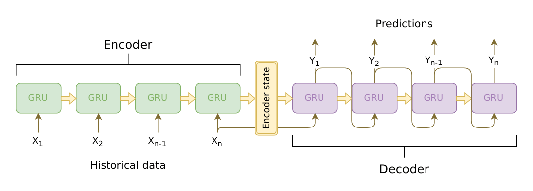
Encoder-decoder is the standard modeling paradigm for sequence-to-sequence tasks. This framework consists of two components:
In this lecture, we'll see different models, but they all have this encoder-decoder structure.
In the Language Modeling lecture, we learned to estimate the probability \(p(y)\) of sequences of tokens \(y=(y_1, y_2, \dots, y_n)\). While language models estimate the unconditional probability \(p(y)\) of a sequence \(y\), sequence-to-sequence models need to estimate the conditional probability p(y|x) of a sequence \(y\) given a source \(x\). That's why sequence-to-sequence tasks can be modeled as Conditional Language Models (CLM) - they operate similarly to LMs, but additionally receive source information \(x\).
Lena : Note that Conditional Language Modeling is something more than just a way to solve sequence-to-sequence tasks. In the most general sense, \(x\) can be something other than a sequence of tokens. For example, in the Image Captioning task, \(x\) is an image and \(y\) is a description of this image.
Since the only difference from LMs is the presence of source \(x\), the modeling and training is very similar to language models. In particular, the high-level pipeline is as follows:
5. Training Protocol, Convergence Behavior & Experimental Evaluation
Similarly to neural classifiers and language models, we can think about the classification part (i.e., how to get token probabilities from a vector representation of a text) in a very simple way. Vector representation of a text has some dimensionality \(d\), but in the end, we need a vector of size \(|V|\) (probabilities for \(|V|\) tokens/classes). To get a \(|V|\)-sized vector from a \(d\)-sized, we can use a linear layer. Once we have a \(|V|\)-sized vector, all is left is to apply the softmax operation to convert the raw numbers into token probabilities.
The simplest encoder-decoder model consists of two RNNs (LSTMs): one for the encoder and another for the decoder. Encoder RNN reads the source sentence, and the final state is used as the initial state of the decoder RNN. The hope is that the final encoder state "encodes" all information about the source, and the decoder can generate the target sentence based on this vector.
This model can have different modifications: for example, the encoder and decoder can have several layers. Such a model with several layers was used, for example, in the paper Sequence to Sequence Learning with Neural Networks - one of the first attempts to solve sequence-to-sequence tasks using neural networks.
In the same paper, the authors looked at the last encoder state and visualized several examples - look below. Interestingly, representations of sentences with similar meaning but different structure are close!
The paper Sequence to Sequence Learning with Neural Networks introduced an elegant trick to make such a simple LSTM model work better. Learn more in this exercise in the Research Thinking section.
Lena : This is the same cross-entropy loss we discussed before in the Text Classification and in the Language Modeling lectures - you can skip this part or go through it quite easily :)
Similarly to neural LMs, neural seq2seq models are trained to predict probability distributions of the next token given previous context (source and previous target tokens). Intuitively, at each step we maximize the probability a model assigns to the correct token.
Formally, let's assume we have a training instance with the source \(x=(x_1, \dots, x_m)\) and the target \(y=(y_1, \dots, y_n)\). Then at the timestep \(t\), a model predicts a probability distribution \(p^{(t)} = p(\ast|y_1, \dots, y_{t-1}, x_1, \dots, x_m)\). The target at this step is \(p^{\ast}=\mbox{one-hot}(y_t)\), i.e., we want a model to assign probability 1 to the correct token, \(y_t\), and zero to the rest.
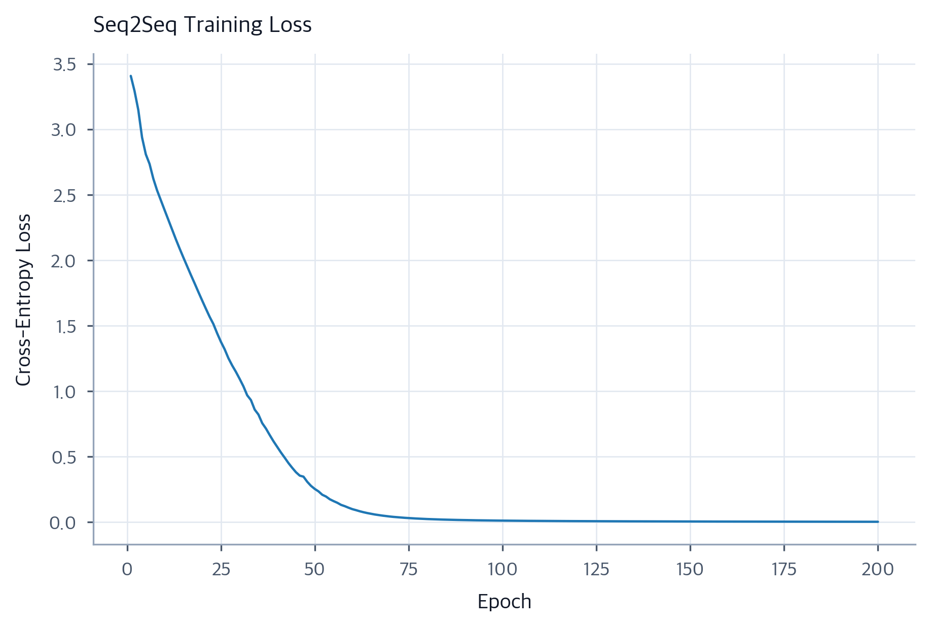
The standard loss function is the cross-entropy loss . Cross-entropy loss for the target distribution \(p^{\ast}\) and the predicted distribution \(p^{}\) is \[Loss(p^{\ast}, p^{})= - p^{\ast} \log(p) = -\sum\limits_{i=1}^{|V|}p_i^{\ast} \log(p_i).\] Since only one of \(p_i^{\ast}\) is non-zero (for the correct token \(y_t\)), we will get \[Loss(p^{\ast}, p) = -\log(p_{y_t})=-\log(p(y_t| y_{\mbox{<}t}, x)).\] At each step, we maximize the probability a model assigns to the correct token. Look at the illustration for a single timestep.
For the whole example, the loss will be \(-\sum\limits_{t=1}^n\log(p(y_t| y_{\mbox{<}t}, x))\). Look at the illustration of the training process (the illustration is for the RNN model, but the model can be different).
Now when we understand how a model can look like and how to train this model, let's think how to generate a translation using this model. We model the probability of a sentence as follows:
Note that we can not find the exact solution. The total number of hypotheses we need to check is \(|V|^n\), which is not feasible in practice. Therefore, we will find an approximate solution.
Model Figures & Evaluation Curves (4 Images)

Deep Learning Execution Pipeline
(Preprocessing)
(Feature Extraction)
(Self-Attention)
(Loss Optimization)