Complete Technical Paper Content — Autonomous Vehicles Ai
1. Executive Abstract, Problem Formulation & Background
EMMA: End-to-End Multimodal Model for Autonomous Driving Jyh-Jing Hwang † † thanks: Equal contributions; ‡ Equal contributions. † † thanks: Contact emails: Mingxing Tan <tanmingxing@waymo.com>, Jyh-Jing Hwang <jyhh@waymo.com>. Runsheng Xu 1 1 footnotemark: 1 Hubert Lin ‡ Wei-Chih Hung ‡ Jingwei Ji Kristy Choi Di Huang Affiliation: Tong He, Paul Covington, Benjamin Sapp, James Guo, Dragomir Anguelov, Mingxing Tan 2 2 footnotemark: 2 Affiliation: Waymo LLC Abstract We introduce EMMA, an End-to-end Multimodal Model for Autonomous driving. Built on a multi-modal large language model foundation, EMMA directly maps raw camera sensor data into various driving-specific outputs, including planner trajectories, perception objects, and road graph elements. EMMA maximizes the utility of world knowledge from the pre-trained large language models, by representing all non-sensor inputs (e.g. navigation instructions and ego vehicle status) and outputs (e.g. trajectories and 3D locations) as natural language text. This approach allows EMMA to jointly process various driving tasks in a unified language space, and generate the outputs for each task using task-specific prompts. Empirically, we demonstrate EMMA’s effectiveness by achieving state-of-the-art performance in motion planning on nuScenes as well as competitive results on the Waymo Open Motion Dataset (WOMD). EMMA also yields competitive results for camera-primary 3D object detection on the Waymo Open Dataset (WOD). We show that co-training EMMA with planner trajectories, object detection, and road graph tasks yields improvements across all three domains, highlighting EMMA’s potential as a generalist model for autonomous driving applications. However, EMMA also exhibits certain limitations: it can process only a small amount of image frames, does not incorporate accurate 3D sensing modalities like LiDAR or radar and is computationally expensive. We hope that our results will inspire further research to mitigate these issues and to further evolve the state of the art in autonomous driving model architectures. 1 Introduction Autonomous driving technology has made significant progress in recent years. To make autonomous vehicles a ubiquitous form of transportation, they must navigate increasingly complex real-world scenarios that require understanding rich scene context as well as sophisticated reasoning and decision-making. Historically, autonomous driving systems employed a modular approach, consisting of specialized components for perception ( Yurtsever et al., 2020 ; Li et al., 2022b ; Lang et al., 2019 ; Sun et al., 2022 ; Hwang et al., 2022 ) , mapping ( Li et al., 2022a ; Tancik et al., 2022 ) , prediction ( Nayakanti et al., 2023 ; Shi et al., 2024 ) , and planning ( Teng et al., 2023 ) . While this design lends itself to easier debugging and optimization of individual modules, it poses scalability challenges due to the accumulated errors among modules and limited inter-module communication. In particular, the expert-designed interfaces between modules, such as the perception and behavior modules, may struggle to adapt to novel environments because they are often pre-defined based on targeted scenarios ( Bansal et al., 2019 ; Jiang et al., 2023 ; Nayakanti et al., 2023 ; Seff et al., 2023 ) . End-to-end autonomous driving systems ( Hu et al., 2023 ; Zhai et al., 2023 ; Li et al., 2024 ) have recently emerged as a potential solution, directly learning to generate driving actions from sensor data. This approach eliminates the need for symbolic interfaces between modules and allows for joint optimization of driving objectives from raw sensor inputs. However, these systems are often specialized for specific driving tasks and trained on limited datasets, hindering their ability to generalize to rare or novel scenarios. Multimodal Large Language Models (MLLMs) ( Gemini Team Google, 2023 ; Achiam et al., 2023 ) offer a promising new paradigm for AI in autonomous driving that may help to address such challenges. This is because MLLMs, as generalist foundation models, excel in two key areas: (1) they are trained on vast, internet-scale datasets that provide rich "world knowledge" beyond what is contained in common driving logs, and (2) they demonstrate superior reasoning capabilities through techniques such as chain-of-thought reasoning ( Wei et al., 2022 ) that are not available in specialized driving systems. While recent efforts ( Chen et al., 2024b ; Tian et al., 2024 ) have explored integrating and augmenting the capabilities of existing driving systems with MLLMs, we propose to develop an autonomous driving system in which the MLLM is a first class citizen. We introduce the E nd-to-End M ultimodal M odel for A utonomous Driving (EMMA), built on top of Gemini ( Gemini Team Google, 2023 ) without additional specialized components. Figure 1 shows the overview of the EMMA framework. EMMA accepts camera images and plain text for other non-vision inputs such as high-level driving commands and historical context. By recasting driving tasks as visual question answering (VQA) problems, EMMA leverages Gemini’s pre-trained capabilities while preserving its extensive world knowledge. After EMMA is fine-tuned with driving logs from all tasks using task-specific prompts (see Figure 2 for more examples), its shared Gemini model generates various driving outputs such as future trajectories for motion planning, perception objects, road graph elements, and scene semantics. Our experiments showcase EMMA’s strong performance on several planning and perception benchmarks despite this simple design. Additionally, we find that EMMA can produce interpretable, human-readable outputs for many perception tasks such as road graph estimation, and is able to function as a generalist model that is both scalable and robust for autonomous driving. Notably, as used here and throughout the paper, the EMMA generalist model refers to a machine learning model that has been trained and fine-tuned on a large volume of driving data to perform a wide range of specific driving tasks in the autonomous driving domain. We summarize our key findings below: 1. EMMA exhibits strong performance in end-to-end motion planning, achieving state-of-the-art performance on public benchmarks nuScenes ( Caesar et al., 2020 ) and competitive results on the Waymo Open Motion Dataset (WOMD) ( Chen et al., 2024a ) . We also show that we can further improve motion planning quality with more internal training data and chain-of-thought reasoning. 2. EMMA demonstrates competitive results for various perception tasks including 3D object detection, road graph estimation, and scene understanding. On the camera-primary Waymo Open Dataset (WOD) ( Hung et al., 2024 ) , EMMA achieves better precision and recall for 3D object detection than state-of-the-art methods. 3. We demonstrate that EMMA can function as a generalist model in the autonomous driving domain, which jointly generates the outputs for multiple driving related tasks. In particular, EMMA matches or even surpasses the performance of individually trained models when it is co-trained with motion planning, object detection, and road graph tasks. 4. Finally, we show EMMA’s capacity to reason and make decisions in complex, long-tail driving scenarios. Despite these promising results, EMMA is not without its limitations. In particular, it faces challenges for real-world deployment due to: (1) limitations in 3D spatial reasoning due to its inability to fuse camera inputs with LiDAR or radar, (2) the need for realistic and computationally expensive sensor simulation to power its closed-loop evaluation, and (3) the increased computational requirements relative to conventional models. We plan to better understand and address such challenges in future work. In the remainder of this paper, Section 2 describes the detailed method of EMMA for end-to-end motion planning and generalist tasks in autonomous driving. In Section 3 , we present experimental results of EMMA on public and internal datasets. Finally, we discuss related works and limitations of our work in Sections 4 and 5 , respectively. 2 Method Figure 1: EMMA overview diagram. It takes 3 inputs ( left ): 1) a high-level command from the router, 2) historical status of the ego vehicle, and 3) surround-view camera videos. The model then predicts ego future trajectories ( right ) for motion planning that will be transformed into vehicle driving control signals. Further, we can ask the model to explain its rationale ( top right ) before predicting trajectories, which enhances both the performance and explainability of the model through chain-of-thought reasoning. Notably, we incorporate visual grounding into the rationale so that the model also predicts the accurate 3D/BEV location for critical objects. For completeness, we highlight three additional capabilities of our model ( bottom ). EMMA is built on top of Gemini ( Gemini Team Google, 2023 ) , a family of MLLMs developed at Google. We leverage the auto-regressive Gemini models that are trained to process interleaved textual and visual inputs to produce text outputs: 𝐎 = 𝒢 ( 𝐓 , 𝐕 ) \mathbf{O}=\mathcal{G}(\mathbf{T},\mathbf{V}) (1) where 𝒢 \mathcal{G} is the Gemini model, 𝐎 \mathbf{O} represents natural language outputs, 𝐓 \mathbf{T} represents natural language prompts, and 𝐕 \mathbf{V} denotes images or videos. The language output 𝐎 = ( o 1 , o 2 , … , o n ) \mathbf{O}=(o_{1},o_{2},...,o_{n}) is generated via next-token prediction, i.e., the output probability can be represented as P ( 𝐎 | 𝐓 , 𝐕 ) = ∏ i = 1 n P ( o i | o < i , 𝐓 , 𝐕 ) P(\mathbf{O}|\mathbf{T},\mathbf{V})=\prod_{i=1}^{n}P(o_{i}|o_{<i},\mathbf{T},\mathbf{V}) for n n output tokens. Our goal is to adapt 𝒢 \mathcal{G} for autonomous driving applications, thereby harnessing the world knowledge obtained during its pre-training phase. As shown in Figure 1 , we map autonomous driving tasks into Gemini-based EMMA formulation. All sensor data are represented as stitched images or videos as 𝐕 \mathbf{V} ; all router commands, driving context, and task-specific prompts are represented as 𝐓 \mathbf{T} ; all output tasks are presented as language outputs 𝐎 \mathbf{O} . A challenge is that many of the inputs and outputs need to capture 3D world coordinates, such as waypoint BEV (Bird’s Eye View) locations ( x , y ) (x,y) for motion planning and the location and size of 3D boxes. We consider two representations: The first is direct text conversion to floating-point numbers, expressed as 𝐓 coordinates = { ( x i , y i ) } ≈ text ( { ( x i , y i ) } ) \mathbf{T_{\text{coordinates}}}=\{(x_{i},y_{i})\}\approx\texttt{text}(\{(x_{i},y_{i})\}) , where the specified decimal precision depends on the distance unit and decimal points. RT-2 ( Brohan et al., 2023 ) exemplifies this approach in robotic control. The second approach uses special tokens to represent each location or action, formulated as 𝐓 coordinates = { ( x i , y i ) } ≈ tokenize ( { ( x i , y i ) } ) \mathbf{T_{\text{coordinates}}}=\{(x_{i},y_{i})\}\approx\texttt{tokenize}(\{(x_{i},y_{i})\}) , with resolution determined by the learned or manually defined discretization scheme. MotionLM ( Seff et al., 2023 ) leverages this method for motion forecasting. We note that the two approaches have their respective strengths and weaknesses. We opt for the text representation such that all tasks can share the same unified language representation space and they can maximally reuse the knowledge from the pre-trained weights, even though the text presentation may produce more tokens than specialized tokenization. 2.1 End-to-End Motion Planning EMMA employs a unified, end-to-end trained model to generate future trajectories for autonomous vehicles directly from sensor data. These generated trajectories are then transformed into vehicle-specific control actions such as acceleration and turning for autonomous vehicles. EMMA’s end-to-end approach aims to emulate human driving behavior, focusing on two critical aspects: (1) first, the use of navigation systems (e.g. Google Maps) for route planning and intent determination, and (2) second, the utilization of past actions to ensure smooth, consistent driving over time. Our model incorporates three key inputs to align with these human driving behaviors: 1. Surround-view camera videos ( 𝐕 \mathbf{V} ): Provides comprehensive environment information. 2. High-level intent command ( 𝐓 intent \mathbf{T}_{\text{intent}} ): Derived from the router, includes directives such as “go straight”, “turn left”, “turn right”, etc . 3. Set of historical ego status ( 𝐓 ego \mathbf{T_{\text{ego}}} ): Represented as a set of waypoint coordinates in Bird’s Eye View (BEV) space, 𝐓 ego = { ( x t , y t ) } t = − 1 − T h \mathbf{T_{\text{ego}}}=\{(x_{t},y_{t})\}_{t=-1}^{-T_{h}} for T h T_{h} timestamps. All waypoint coordinates are represented as plain text without specialized tokens. This can also be extended to include higher-order ego status such as velocity and acceleration. The model generates future trajectories for motion planning, represented as a set of future trajectory waypoints for the ego vehicle in the same BEV space: 𝐎 trajectory = { ( x t , y t ) } t = 1 T f \mathbf{O_{\text{trajectory}}}=\{(x_{t},y_{t})\}_{t=1}^{T_{f}} for future T f T_{f} timestamps, where all output waypoints are also represnted as plain text. Putting everything together, the complete formulation is expressed as: 𝐎 trajectory = 𝒢 ( 𝐓 intent , 𝐓 ego , 𝐕 ) . \mathbf{O_{\text{trajectory}}}=\mathcal{G}(\mathbf{T_{\text{intent}}},\mathbf{T_{\text{ego}}},\mathbf{V}). (2) We then fine-tune Gemini with this formulation for end-to-end planner trajectory generation, as illustrated in Figure 1 . We highlight 3 characteristics of this formulation: 1. Self-supervised : the only required supervision is the future locations of the ego vehicle. No dedicated human labels are needed. 2. Camera-only : the only sensor input required is surround-view cameras. 3. HD map free : no HD map is needed beyond the high-level routing information from a navigation system such as Google Maps. While we are not the first to adopt this general formulation— ( Li et al., 2024 ) conducted a thorough investigation, particularly examining the impact of including the historical ego status—our contribution lies in adapting this formulation specifically for MLLMs for autonomous driving. 2.2 Planning with Chain-of-Thought Reasoning Chain-of-thought Prompting ( Wei et al., 2022 ) is a powerful tool in MLLMs that enhances reasoning capabilities and improves explainability. In EMMA, we incorporate chain-of-thought reasoning into end-to-end planner trajectory generation by asking the model to articulate its decision rationale 𝐎 rationale \mathbf{O_{\text{rationale}}} while predicting the final future trajectory waypoints 𝐎 trajectory \mathbf{O_{\text{trajectory}}} . We structure the driving rationale hierarchically, progressing from 4 types of coarse-to-fine-grained information: R1 - Scene description broadly describes the driving scenarios, including weather, day of time, traffic situations, and road conditions. For example: The weather is clear and sunny, and it is daytime. The road is four-lane undivided street with a crosswalk in the middle. There are cars parked on both sides of the street. R2 - Critical objects are the on-road agents that can potentially influence the driving behavior of the ego vehicle, and we require the model to identify their precise 3D/BEV coordinates. For instance: pedestrian at [9.01, 3.22], vehicle at [11.58, 0.35] . R3 - Behavior description of critical objects describes the current status and intent for the identified critical objects. A concrete example is as follows: The pedestrian is currently standing on the sidewalk, looking toward the road, and maybe preparing to cross the street. The vehicle is currently ahead of me, moving in the same direction, and its future trajectory suggests it will continue straight. R4 - Meta driving decision includes 12 categories of high-level driving decisions, summarizing the driving plan given the previous observations. An example would be I should keep my current low speed . We highlight that the driving rationale captions are generated using an automated tool without any additional human labels, ensuring scalability of the data generation pipeline. Specifically, we leverage off-the-shelf perception and prediction expert models to identify critical agents, and then use Gemini models with carefully designed visual and text prompts to generate comprehensive scene and agent behavior descriptions. Meta driving decisions are computed using a heuristic algorithm that analyzes the ego vehicle’s ground-truth trajectory. During both training and inference, the model predicts all four components of the driving rationale before predicting the future waypoints, i.e., ( 𝐎 rationale , 𝐎 trajectory ) = 𝒢 ( 𝐓 intent , 𝐓 ego , 𝐕 ) . (\mathbf{O_{\text{rationale}}},\mathbf{O_{\text{trajectory}}})=\mathcal{G}(\mathbf{T_{\text{intent}}},\mathbf{T_{\text{ego}}},\mathbf{V}). (3) Where 𝐎 rationale \mathbf{O_{\text{rationale}}} denotes an ordered text output of (R1, R2, R3, R4) for driving rationale. Empirically, we observe that the prediction order of 𝐎 rationale \mathbf{O_{\text{rationale}}} and 𝐎 trajectory \mathbf{O_{\text{trajectory}}} does not result in a significant difference in quality after model convergence. This suggests that we can predict 𝐎 trajectory \mathbf{O_{\text{trajectory}}} first and apply early stopping during inference for time-critical applications. 2.3 EMMA Generalist While end-to-end motion planning is the ultimate core task, a comprehensive autonomous driving system requires additional capabilities. Specifically, it must perceive the 3D world and recognize surrounding objects, the road graph and the traffic conditions. To achieve this goal, we formulate EMMA as a generalist model capable of handling multiple driving tasks through training mixtures. Our vision-language framework represents all non-sensor inputs and outputs as plain text, providing the flexibility necessary to incorporate many other driving tasks. We employ instruction-tuning, a well-established approach in LLMs, to jointly train all tasks together with task-specific prompts included in the inputs 𝐓 \mathbf{T} of Eq. 1 . We organize these tasks into three primary categories: spatial reasoning, road graph estimation, and scene understanding. Fig. 2 illustrates the overall EMMA Generalist diagram. Spatial reasoning is the ability to understand, reason, and draw conclusions about objects and their relationships in space. This enables an autonomous driving system to interpret and interact with its surrounding environment for safe navigation. Our primary focus for spatial reasoning is 3D object detection. We follow Pix2Seq ( Chen et al., 2022a ) and formulate the output 3D bounding boxes as 𝐎 boxes = set { text ( x , y , z , l , w , h , θ , cls ) } \mathbf{O}_{\text{boxes}}=\texttt{set}\{\texttt{text}(x,y,z,l,w,h,\theta,\textit{cls})\} where ( x , y , z ) (x,y,z) are the center location in the vehicle frame, l , w , h l,w,h are the length, width, and height of the box, θ \theta is the heading angle, and cls is the class label in text. We convert a 7D box to text by writing floating-point numbers with two decimal places, separated by spaces between each dimension. Figure 2: Illustration of EMMA Generalist. Starting with a task prompt ( left ), EMMA generates a corresponding textual prediction ( middle right ), which can then be decoded into a target output format, visualized and overlaid with the input image ( right ). EMMA Generalist is highly versatile, capable of performing a wide range of driving-related tasks, such as end-to-end motion planning, object detection, road graph estimation, and scene understanding Q&A. In the answer text, italicized words represent placeholders that will be dynamically substituted with actual values during task execution. We then represent the detection tasks using a fixed prompt 𝐓 detect_3D \mathbf{T_{\text{detect\_3D}}} , such as “ detect every object in 3D ”, as in the following: 𝐎 boxes = 𝒢 ( 𝐓 detect_3D , 𝐕 ) . \mathbf{O_{\text{boxes}}}=\mathcal{G}(\mathbf{T_{\text{detect\_3D}}},\mathbf{V}). (4) While 𝐎 boxes \mathbf{O_{\text{boxes}}} is an unordered set of boxes, the predictions from an auto-regressive language model are always ordered. We find that sorting the 3D bounding boxes by depth improves detection quality, in contrast with the findings in Pix2Seq ( Chen et al., 2022a ) . Road graph estimation focuses on identifying critical road elements for safe driving, including semantic elements (e.g., lane markings, signs) and physical properties (e.g., lane curvature). The collection of these road elements forms a road graph. For example, lane segments are represented by (a) nodes, where the lanes encounter an intersection, merge, or split and (b) edges between these nodes following the direction of traffic. The full road-graph is composed of many such polyline segments. While edges within each polyline are directional, each polyline does not necessarily have a unique order relative to the other elements. This bears similarity to object detection (e.g., ( Carion et al., 2020 ; Chen et al., 2022a ) ), where each box is defined by ordered attributes (top-left corner, bottom-right corner), but a relative ordering between boxes does not necessarily exist. There are several existing works that model polyline graphs with Transformers ( Yuan et al., 2024 ; Liao et al., 2024a ; Liao et al., 2024b ; Liao et al., 2023 ; Ding et al., 2023 ; Qiao et al., 2023 ; Liu et al., 2023 ; Li et al., 2022a ) , sharing similarities with language models. Our general modeling formulation in EMMA is as follows: 𝐎 roadgraph = 𝒢 ( 𝐓 estimate_roadgraph , 𝐕 ) . \mathbf{O_{\text{roadgraph}}}=\mathcal{G}(\mathbf{T_{\text{estimate\_roadgraph}}},\mathbf{V}). (5) where 𝐎 roadgraph \mathbf{O_{\text{roadgraph}}} is a text-encoded road graph represented as waypoints, 𝐓 estimate_roadgraph \mathbf{T_{\text{estimate\_roadgraph}}} is a prompt asking the model to predict the roadgrah, and 𝐕 \mathbf{V} denotes the surrounding images. We focus specifically on predicting drivable lanes, i.e., the lanes that the ego vehicle can drive towards in the scene. These are neighboring lanes in the same traffic direction and lanes branching out from the current ego lane. To construct 𝐎 roadgraph \mathbf{O}_{\text{roadgraph}} , we (a) convert lanes into sets of ordered waypoints and (b) transform these sets of waypoints into text. It is beneficial to use sample-ordered waypoints to represent both traffic direction and curvature. Just like detection, we also find that ordering lanes by approximate distance improves the prediction quality. An example of our polyline text encoding is: "(x1,y1 and... and xn,yn);..." where "x,y" are floating point waypoints with precision to 2 decimal places, ";" separates polyline instances. Scene understanding tasks test the model’s understanding of the whole scene context, which can be relevant for driving. For example, roads can be temporarily obstructed due to construction, emergency situations, or other events. Detecting these blockages in a timely manner and safely navigating around them is essential for ensuring the smooth and safe operation of autonomous vehicles; however, multiple cues in the scene are required to determine if there is a blockage or not. We focus on how our model performs on this temporary blockage detection task, using the following formulation: 𝐎 temporary_blockage = 𝒢 ( 𝐓 temporary_blockage , 𝐓 road_user , 𝐕 ) , \mathbf{O_{\text{temporary\_blockage}}}=\mathcal{G}(\mathbf{T_{\text{temporary\_blockage}}},\mathbf{T_{\text{road\_user}}},\mathbf{V}), (6) where 𝐎 temporary_blockage \mathbf{O_{\text{temporary\_blockage}}} is the model output signaling potential obstruction, 𝐕 \mathbf{V} denotes the surrounding images, 𝐓 road_users \mathbf{T_{\text{road\_users}}} denotes the all the objects on the road ahead, 𝐓 temporary_blockage \mathbf{T_{\text{temporary\_blockage}}} is the text prompt "is the road ahead temporarily blocked?" . 2.4 Generalist Training Our unified vision-language formulation enables the simultaneous training of multiple tasks with a single model, allowing for task-specific predictions at inference time through simple variations of the task prompt 𝐓 task \mathbf{T}_{\text{task}} . The training procedure is both straightforward and flexible. For each task, we construct a dataset 𝐃 task \mathbf{D}_{\text{task}} containing | 𝐃 task | |\mathbf{D}_{\text{task}}| training examples. During each training iteration, we randomly sample a batch from the available datasets, with the probability of selecting an example from a specific dataset proportional to the dataset size: i.e. , | 𝐃 task | / ∑ t | 𝐃 t | |\mathbf{D}_{\text{task}}|/\sum_{t}|\mathbf{D}_{\text{t}}| . To train for e e epochs, we set the total number of training iterations to e × ∑ t | 𝐃 t | e\times\sum_{t}|\mathbf{D}_{\text{t}}| , ensuring that the training ratio among tasks is governed by the relative dataset sizes. The optimal training ratio is influenced by several factors, including task complexity, inter-task correlations, and the degree of transferability across tasks. Our experimental results demonstrate that the generalist model, trained across multiple tasks, consistently outperforms each specialist model that is trained on a single task. This highlights the advantage of the generalist approach: enhanced knowledge transfer, improved generalization, and increased efficiency. 3 Experiments We highlight the experiments used to validate the efficacy of EMMA model. We leverage the smallest size of Gemini, i.e., Gemini 1.0 Nano-1 ( Gemini Team Google, 2023 ) for all the experiments. In the following section, we first present the results of end-to-end planner trajectory generation on two public datasets in Section 3.1 . Next, we conduct additional experiments on our internal datasets, studying the impact of chain-of-thought and data scaling in Section 3.2 . Section 3.3 focuses on experiments involving three core perception tasks: 3D object detection, road graph estimation, and scene understanding. Our co-training results for the generalist model are summarized in Section 3.4 . Finally, we showcase visual results that highlight EMMA capabilities in challenging, long-tail scenarios in Section 3.5 . 3.1 End-to-End Motion Planning on Public Datasets We conduct the end-to-end planner trajectory generation experiments on two public datasets, the Waymo Open Motion Dataset (WOMD) ( Chen et al., 2024a ) and the nuScenes dataset ( Caesar et al., 2020 ) . EMMA is trained with the simplest end-to-end planner trajectory generation formulation as in Equation 2 . That is, given camera images, ego vehicle history, and driving intent, the model is asked to predict the future ego waypoints for a certain time horizon. Method ADE 1s ADE 3s ADE 5s ADE 8s MotionLM ( Seff et al., 2023 ) 0.045 0.251 0.694 1.766 Wayformer* ( Nayakanti et al., 2023 ) 0.044 0.250 0.640 1.517 EMMA 0.032 0.248 0.681 1.718 EMMA+ 0.030 0.225 0.610 1.553 Table 1: End-to-end motion planning experiments on WOMD ( Chen et al., 2024a ) . EMMA+ denotes the models are pre-trained on our internal data. EMMA achieves state-of-the-art performance on the WOMD planning benchmark to ADE 1s, 3s, and 5s. EMMA is slightly worse than Wayformer at ADE 8s, largely because the camera-only EMMA has higher depth error for longer distance than Wayformer, which uses all sensors including LiDAR, Radar, and Cameras. ∗ Note that the Wayformer baseline is based on an enhanced internal version after the publication of ( Nayakanti et al., 2023 ) . Figure 3: Ablation study on the number of sampled trajectories. As more trajectories are sampled, the quality measured by ADE@5s also improves, but the benefits diminish after 12+ samples. 3.1.1 Driving on the Waymo Open Motion Dataset (WOMD) WOMD comprises 103k real-world urban and suburban driving scenarios, each lasting 20 seconds. These scenarios are further segmented into 1.1M examples, each representing a 9-second window: 1 second is used as input context, and the remaining 8 seconds serve as the prediction target. The dataset includes detailed map features such as traffic signal states and lane characteristics, along with agent states such as position, velocity, acceleration, and bounding boxes. WOMD is typically used for the agent motion prediction task, i.e., given the agent tracks for the past 1 second on a corresponding map, predict the positions of up to 8 agents for 8 seconds into the future. We adopt the exact same setting but only evaluate the future motion prediction of the ego vehicle as the planning benchmark. In addition, we leverage the ‘intent’ field, used for evaluating motion prediction, as the planning router instruction. We adapt some of the best motion prediction models, MotionLM ( Seff et al., 2023 ) and enhanced Wayformer ( Nayakanti et al., 2023 ) , as the baselines of this planning benchmark. During inference, sampling a final trajectory from multiple candidate trajectories plays a critical role in the final performance. Both MotionLM and Wayformer generate 192 candidate trajectories, which are subsequently aggregated into 6 clusters using k-means clustering, resulting in 6 representative trajectories. The final trajectory is selected from these 6 representative trajectories based on their associated probabilities. For fairness, we also sample multiple trajectories using a Top- K K decoding strategy, up to K = 24 K=24 . We then compute the pairwise L2 distance between all trajectories and select the one with the lowest average L2 distance as the final predicted trajectory, which can be viewed as the “median” trajectory among all the predictions. In the ADE calculation, we treat this median trajectory with the highest probability. As shown in Table 1 , our model achieved similar performance as the MotionLM baseline when we train only on the WOMD dataset, with Gemini pre-trained weights. When pre-trained with our internal dataset (denoted as EMMA+), our model surpasses both MotionLM and Wayformer up to ADE 5s in the future. EMMA is only slightly worse than Wayformer at ADE 8s, where camera-induced depth error becomes a prominent error resource. We note the differences in inputs between MotionLM and EMMA: MotionLM takes inputs of agent location history, agent interactions, the road graph, and traffic light states. These agent boxes are produced by specialized off-board perception models that look at both past and future observations and are trained with a large amount of carefully curated human labels, the road graph is manually generated using full run segments, and all inputs heavily use LiDAR data with superior depth estimation. In stark contrast, EMMA only takes camera images and ego vehicle history as input, without the need of any labels or additional models (besides leveraging the Gemini pre-trained weights). Notably, for this work, we added internally available image inputs, which are not currently in the released WOMD. We further investigate the impact of the number of sampled trajectories on ADE, as illustrated in Figure 3 . The results highlight that sampling from multiple trajectories, rather than a single one, leads to a notable improvement in ADE. However, the advantage of increasing the number of candidate trajectories diminishes beyond a certain point. 3.1.2 Driving on the nuScenes Dataset The nuScenes dataset ( Caesar et al., 2020 ) offers a comprehensive autonomous vehicle sensor suite for evaluation. It consists of 1,000 scenes, each spanning 20 seconds, and includes information from 6 cameras, 5 radars, and 1 LiDAR that collectively provide 360-degree coverage in the field of view. The dataset is fully annotated with 3D bounding boxes across 23 classes and 8 attributes. In our experiments, we follow the standard protocol for planning evaluation: predict the next 3 seconds of future driving actions based on 2 seconds of historical data. We measure the planning quality with L2 errors at 1-, 2- and 3-second time horizons, aligning with established baseline methods. As shown in Table 2 , our self-supervised EMMA achieves state-of-the-art results in planning on nuScenes, outperforming all previous supervised (with intermediate perception labels and/or human labels) and self-supervised (no extra labels) methods. Under the same self-supervised setup, EMMA outperforms previous BEV-Planner ( Li et al., 2024 ) by 17.1% in average L2 metric; even compared to DriveVLM-Dual ( Tian et al., 2024 ) that heavily uses intermediate perception and human labels, our self-supervised EMMA still improves the average L2 metric by 6.4%. Unlike in WOMD, we note that sampling multiple trajectories did not yield significant improvements. We hypothesize that this is due to nuScenes’ shorter prediction time horizon (3s) in simpler driving scenarios. Thus, we report only top-1 predictions for our results. Method self-supervised? L2 (m) 1s L2 (m) 2s L2 (m) 3s Avg L2 (m) UniAD ( Hu et al., 2023 ) ✗ 0.42 0.64 0.91 0.66 DriveVLM ( Tian et al., 2024 ) ✗ 0.18 0.34 0.68 0.40 VAD ( Jiang et al., 2023 ) ✗ 0.17 0.34 0.60 0.37 OmniDrive ( Wang et al., 2024a ) ✗ 0.14 0.29 0.55 0.33 DriveVLM-Dual ( Tian et al., 2024 ) ✗ 0.15 0.29 0.48 0.31 Ego-MLP ∗ ( Zhai et al., 2023 ) ✓ 0.15 0.32 0.59 0.35 BEV-Planner ( Li et al., 2024 ) ✓ 0.16 0.32 0.57 0.35 EMMA (random init) ✓ 0.15 0.33 0.63 0.37 EMMA ✓ 0.14 0.29 0.54 0.32 EMMA+ ✓ 0.13 0.27 0.48 0.29 Table 2: End-to-end motion planning experiments on nuScenes ( Caesar et al., 2020 ) . EMMA (random init) denotes models are randomly initialized; EMMA denotes models are initialized from Gemini; EMMA+ denotes models are pre-trained on our internal data. EMMA achieves state-of-the-art performance on the nuScenes planning benchmark, outperforming the supervised (with perception and/or human labels) prior art by 6.4% and self-supervised (no extra labels) prior art by 17.1%. ∗ Ego-MLP results are taken from a reproduced version in BEV-Planner. 3.2 End-to-End Motion Planning with Chain-of-Thought Reasoning on Internal Dataset In this section, we present our studies of end-to-end planning with chain-of-thought on our internal dataset. This dataset contains millions of scenarios, orders of magnitude larger than any publicly available autonomous driving dataset. The model takes in 2 seconds of history to predict the driving actions for 5 seconds into the future. Table 3 presents the results of our experiments on chain-of-thought reasoning applied to end-to-end planning. By adopting the chain-of-thought formulation introduced in Equation 3 , we achieve a notable 6.7% improvement over the standard end-to-end planning approach detailed in Equation 2 . We also conduct an ablation study to analyze the contributions of different rationale components. Our findings reveal that both driving meta-decision and critical object identification significantly enhance performance, contributing improvements of 3.0% and 1.5%, respectively. When these components are combined, the gains are even more substantial. Conversely, while scene description has a neutral impact on driving performance, it enhances the model’s explainability. These results demonstrate that chain-of-thought reasoning can meaningfully improve driving performance, particularly when its components are carefully selected and integrated. Scene description Critical object Meta decision Behavior description Relative improvements over baseline e2e planning ✓ ✗ ✗ ✗ + 0.0% ✗ ✓ ✗ ✗ + 1.5% ✗ ✗ ✓ ✗ + 3.0% ✗ ✓ ✓ ✗ + 5.7% ✗ ✓ ✓ ✓ + 6.7% Table 3: Ablation study on chain-of-thought reasoning components. It improves end-to-end planning quality by up to 6.7% by combining all elements. In particular, driving meta-decision and critical objects contribute the improvements of 3.0% and 1.5%, respectively. The details of each component is described in Section 2.2 . We also perform a series of data scaling experiments for end-to-end planning, the results of which are illustrated in Figure 4 . As we train the model on a larger training set, we observe lower eval perplexities before overfitting. Our findings indicate that the driving quality of EMMA has not yet plateaued, even with the current large-scale dataset. Figure 4: EMMA data scaling experiments on our internal dataset. Each curve represents the eval perplexity for end-to-end motion planning as training proceeds with more steps. The x-axis is training compute, measured by floating-point operations (FLOPs) in log scale. The same EMMA model is trained on four sizes of datasets that are sampled with different percentages from 3% to 100% (denoted by different colors). In general, EMMA tends to achieve better quality until overfitting when given more training compute, but it also overfits quickly on smaller datasets. We observe the driving quality has not saturated when using the full large-scale dataset. 3.3 Perception Tasks We summarize our studies on three main perception tasks: 3D object detection, road graph estimation, and scene understanding. 3.3.1 3D Object Detection We validate our 3D object detection performance on the 3D camera-primary detection benchmark from the Waymo Open Dataset ( Sun et al., 2020 ) using the d Longitudinal Error Tolerant (LET) matching ( Hung et al., 2024 ) . We evaluate two versions: EMMA and EMMA+, similar to earlier sections, where EMMA+ is pre-trained on the 3D detection task using our internal dataset. The quantitative results are reported on the official test set and summarized in Figure 5 . Figure 5: Camera-primary 3D object detection experiments on WOD ( Sun et al., 2020 ) using the standard LET matching ( Hung et al., 2024 ) . EMMA+ denotes model is pre-trained on our internal data. EMMA+ achieves competitive performance on the detection benchmark in both precision/recall and F1-score metrics. Compared to state-of-the-art methods, it achieves 16.3% relative improvements in vehicle precision at the same recall or 5.5% recalls improvement at the same precision. Our findings show that after pre-training, EMMA+ achieves competitive performance on the benchmark. Since our model output set of detected boxes without individual confidence scores, we directly compare the precision/recall instead of LET-3D-AP, which is calculated based on the precision/recall curve. We also compare the commonly used F1-score, where EMMA’s F1-score is computed using the single precision/recall and other models’ F1-scores are calculated by picking the maximal F1-score on the curve (often called F1-max). Figure 5 shows the performance comparison. In generally, EMMA+ demonstrates substantial improvements over state-of-the-art methods such as BEVFormer ( Li et al., 2022b ) , achieving a 16.3% relative increase in vehicle precision at the same recall, and a 5.5% recall improvement at the same precision. EMMA+ also achieve better F1-score than prior arts. Performance on the pedestrian class is also comparable to that of MV-FCOS3D++ ( Wang et al., 2021 ) . Additionally, we provide a performance breakdown across different ranges, highlighting that our model performs especially well in the near range. Our results underscore that with sufficient data and a large enough model, a multimodal approach can surpass specialized expert models in 3D object detection quality. 3.3.2 Road Graph Estimation Road graph estimation is a complex task that predicts a group of unordered polylines, each of which is represented as a sequence of waypoints. We measure the quality of road graph prediction with two metrics: (1) lane-level precision and recall, where we define a true positive match between a predicted lane polyline and a groundtruth lane polyline if and only if their Chamfer distance is within 1 meter; and (2) pixel-level precision and recall, where polylines are rasterized into a BEV grid with 1 meter resolution – we then treat the BEV grid as a image and compute precision and recall based on per-pixel matching. As discussed in Section 2.3 , this task involves several design choices. One is about the representation of road graph polylines, where our choice is to define the start and end points of each lane, with intermediate points added as needed to accurately capture the road’s curvature. Another critical design choice is the construction of target label sequences used for model training. Drawing inspiration from Pix2Seq ( Chen et al., 2022a ) in the context of object detection, one effective design choice is to pad the targets and apply random shuffling. This technique helps the model handle unordered outputs and prevents premature termination during training. Figure 6 presents our ablation studies on various design choices. Starting from our best designs, we systematically ablate each of the following configurations and assess the resulting quality degradation. We then summarize the key insights from our analysis. Polyline representation: dynamic sampling is better than fixed sampling . A simple polyline representation is to sample a fixed number of sparse control points per lane, e.g. two end points plus a fixed number of intermediate points to capture curvature. However, we find a better approach is to dynamically adjust the number of points per polyline according to the curvature and length of the lane. By keeping a consistent waypoint density rather than a consistent number of waypoints, we achieve a representation that more accurately captures the lane structure intricacies, yielding around a 40% to 90% difference in the metrics as shown in Figure 6 . Polyline representation: ego-origin aligned sample intervals are better than naively aligned sample intervals . The road graph is typically stored and accessed in global coordinate frame, meaning lane origins and extensions are independent of the ego vehicle position. To improve accuracy, it is essential to adjust lane point samples to start from the ego vehicle coordinate frame origin. Specifically, sampling polyline points relative to the AV position (ego-origin) avoids arbitrary offsets that can arise from directly transforming points sampled in the global coordinate frame into the ego coordinate frame. This prevents a 25% to 60% drop in prediction quality. Target sequence construction: shuffled ordering is better than arbitrary ordering . We organize polyline targets into bins based on their endpoint distance from the ego vehicle, providing a rough global ordering. For instance, we categorize lanes into nearby lanes and those further away that serve as connecting lanes. During training, we dynamically shuffle the polylines within each distance bin to enhance the model robustness and coverage. This dynamic shuffling within each bin improves the model’s ability to generalize across different lane configurations, leading to more accurate predictions. Target sequence construction: padding is better than non-padding . Similar to Pix2Seq ( Chen et al., 2022a ) , we find that padding targets to prevent early termination is highly effective. In addition to padding the total number of polyline targets, we also pad the number of points within each polyline. We use “invalid” tokens to represent padded points within polylines. Each polyline is also explicitly tagged with a final “valid” or “invalid” token to denote whether it contains any nonpadded points. This approach ensures consistent input sizes, which helps maintain the integrity of the model during training and reduces the risk of premature truncation, leading to more reliable and accurate predictions. Target sequence construction: adding punctuation and other semantically redundant token improves quality . In the target sequence construction, we notice that it is beneficial to use language-like structures and punctuation to group targets (e.g., "(x,y and x,y);..." instead of "xy xy;...") . Additionally, explicitly including semantically redundant tokens – such as marking padded targets as “invalid” instead of relying on implicit omissions of “valid” markers – improves performance. This approach, incorporating punctuation and redundancy, results in a boost of up to 10% in lane-level metrics. We attribute this improvement to the language-related pre-training of Gemini. By leveraging similar structured expressions, Gemini can be more easily adapted to other tasks. Figure 6: Ablation study on road graph estimation. To evaluate the influence of different components in our road graph estimation model, we ablate each configuration and measure the corresponding impact on quality. Dynamic sampling ( leftmost ) of road graph polylines based on lane curvature and length proves to be the most significant factor, leading to a substantial 70% to 90% change in lane-level precision and recall. In contrast, aligning the model with a language-like representation, i.e. , semantic punctuation ( rightmost ), has a more modest effect, contributing to only <10% change in precision and recall of any metric. 3.3.3 Scene Understanding Figure 7 summarizes our studies on the scene understanding task for temporary blockage detection . Our study is based on our internal datasets specifically curated for these scenarios. For this study, we establish our baselines by showing a picture to human and asking them to judge whether a lane is temporarily blocked. They can answer ‘yes’, ‘no’, or ‘unsure’. Our baseline will treat all ‘unsure’ answers as incorrect, baseline+filtering will filter out all examples with ‘unsure’ answers. In contrast, our model is fine-tuned to predict ‘yes’ or ‘no’ for all examples. As shown in the figure, our naive model that is directly fine-tuned for only this task achieves better performance than the baseline comparison, but underperforms on the baseline+filtering comparison. To boost the model performance, our first attempt is to co-train this task with road graph estimation, but the naive mixture doesn’t improve performance. Our second attempt is to first pre-train the model on road graph estimation, and then fine-tune on these two tasks. Results show when the pre-training is long enough, the quality is boosted, showcasing the model’s ability to integrate multiple tasks for enhanced performance. Figure 7: Scene understanding experiments. direct fine-tuning denotes solely using the temporal blockage data during fine-tuning; naive mixture denotes co-training this scene task with road graph estimation; mix + short pretraining denotes pre-training on road graph esitmation first, and then fine-tune on the mixture of both tasks; mix + long pretraining denotes a longer pre-training before fine-tuning. The naive fine-tuning is already close to strong human baseline, but long-pretraining with training mixture can further boost the quality. 3.4 Generalist We explore the development of a generalist model by co-training on multiple tasks and analyzing their synergies, as summarized in Table 4 . For this study, we focus on three core tasks: end-to-end planning, 3D object detection, and road graph estimation. Co-training on all three tasks yields significant improvements, with the generalist model outperforming the single-task models by up to 5.5%. Notably, when co-training two tasks, certain combinations lead to greater gains than others. For instance, detection performance improves most when co-trained with driving, and road graph estimation similarly benefits most when paired with driving. This suggests that the driving task plays a particularly prominent and influential role, serving as a key contributor to overall performance improvements. We attribute these results to the complementary nature of the tasks. For example, road graph estimation becomes easier when the model can accurately identify the locations of vehicles. Similarly, driving quality is closely tied to understanding agent interactions, a skill enhanced by 3D object detection. These findings suggest that pursuing a generalist model is a promising direction for future research, with the potential for deeper insights into task synergies and performance optimization. Relative improvement over single task e2e planning 3D detection road graph estimation e2e planning detection road graph ✓ ✓ - +1.6% ( ± \pm 1.0%) +2.4% ( ± \pm 0.8%) ✓ ✓ +1.4% ( ± \pm 2.8%) +5.6% ( ± \pm 1.1%) - ✓ ✓ − - 1.4% ( ± \pm 2.9%) - +3.5% ( ± \pm 0.9%) ✓ ✓ ✓ +1.4% ( ± \pm 2.8%) +5.5% ( ± \pm 1.1%) +2.4% ( ± \pm 0.8%) Table 4: Generalist co-training experiments. ( ± ∗ \pm* ) indicates standard deviation. By co-training on multiple tasks, EMMA gains a broader understanding of driving scenes, enabling it to handle various tasks at inference time, while enhancing individual task performance. Notably, certain task pairings yield greater benefits than others, suggesting these tasks are complementary. Co-training all three tasks together yields the best quality. 3.5 Visualizations We present 12 diverse visual examples in Fig. 8 , 9 and 10 , each selected to highlight the generalizability of EMMA model across a range of scenarios. In all the scenarios, we display the model’s predictions (from left to right): end-to-end motion planning, 3D object detection, and road graph estimation. We group visual examples by scenario type: Examples (a)-(d) showcase how EMMA safely interacts with rare, unseen objects or animals on the road. Examples (e)-(f) feature EMMA navigating through construction areas. Examples (g)-(j) showcase EMMA following traffic rules at intersections with traffic lights or traffic controllers. Examples (k)-(l) highlight EMMA respecting vulnerable road users like motorcyclists. Given these examples, we demonstrate the following capabilities of EMMA: • Generalizability : Adapts well to diverse real-world driving scenarios across different environments and attends to objects beyond its fine-tuning categories, such as squirrels. • Predictive driving : Proactively adjusts to the behavior of other road users for safe and smooth driving. • Obstacle avoidance : Consistently adjusts trajectories to avoid obstacles, debris and blocked lanes. • Adaptive behavior : Safely handles complex situations like yielding, construction zones, and following traffic control signals. • Accurate 3D detection : Effectively identifies and tracks road agents, including vehicles, cyclists, motorcyclists, and pedestrians. • Reliable road graph estimation : Accurately captures road layouts and integrates them into safe trajectory planning. To conclude, these scenarios highlight EMMA’s capability to operate safely and efficiently in a variety of challenging and diverse driving scenarios and environments. (a) A garbage bag appears on the freeway, so our predicted trajectory suggests to nudge slightly to the right to avoid it. (b) A ladder appears on the freeway, and our predicted trajectory suggests to switch to the left lane to bypass it appropriately. (c) we encounter a small squirrel on the road and our predicted trajectory instinctively slows down to avoid the animal. Note EMMA wasn’t explicitly trained to detect squirrels. (d) A white dog appears in our lane, and our model predicts to slow down and yield. Our model also accurately detects surrounding vehicles, including those in adjacent lanes and the parking lot. Figure 8: EMMA prediction visualization. Each row contains a scenario with our model’s predictions: end-to-end planning (left), 3D object detection (middle), and road graph estimation (right). (e) As a construction zone blocks the left lanes, our predicted trajectory suggests passing through on the right, while the road graph estimation correctly identifies the blocked area. (f) Our lane is blocked by construction cones, so our predicted trajectory suggests to move into the left lane, even though it’s in the opposite direction. EMMA captured the blockage and performed a safe detour. (g) A traffic controller signals to proceed through the intersection, and our predicted trajectory aligns with the instruction. (h) Our predicted trajectory suggests to stop as we approach an intersection with a yellow light, demonstrating cautious and safe behavior. Figure 9: EMMA prediction visualization. Each row contains a scenario with our model’s predictions: end-to-end planning trajectory (left), 3D object detection (middle), and road graph estimation (right). (i) While crossing an intersection, our predicted trajectory nudges slightly to the left due to nearby cars and a bicyclist partially occupying our lane. (j) Our model predicts a driving trajectory to patiently wait at a red light (left). The model also accurately predicts surrounding 3D objects (middle) and road graph with lane centers (right). (k) A fleet of fast-moving motorcyclists passes by. The predicted trajectory suggests pausing to allow them to pass safely. Notably, motorcyclists are accurately identified by our model (middle). (l) A motorbike is moving on a narrow lane at night, and yields to the right. Our predicted trajectory adjusts, guiding us to pass safely by nudging slightly to the left. Figure 10: EMMA prediction visualization. Each row contains a scenario with our model’s predictions: end-to-end planning trajectory (left), 3D object detection (middle), and road graph estimation (right). 4 Related Works End-to-end autonomous driving research enjoys a rich history and has evolved significantly since ALVINN ( Pomerleau, 1988 ) employed shallow neural networks to predict control signals. The field benefited from further deep learning advancements: e.g. DAVE-2 ( Bojarski et al., 2016 ) and ChauffeurNet ( Bansal et al., 2019 ) , leveraged deeper neural architectures and incorporated sophisticated perception and motion planning modules respectively. Recent research has expanded to include multimodal inputs ( Codevilla et al., 2018 ; Prakash et al., 2021 ) , multi-task learning ( Chitta et al., 2022 ; Wu et al., 2022 ) , reinforcement learning ( Chekroun et al., 2023 ; Chen et al., 2021 ; Kendall et al., 2019 ; Liang et al., 2018 ; Toromanoff et al., 2020 ) , and distillation ( Chen et al., 2020 ; Zhang and Ohn-Bar, 2021 ; Zhang et al., 2021 ) . Unified planning frameworks such as VAD ( Jiang et al., 2023 ) and UniAD ( Hu et al., 2023 ) integrated planning with conventional modules in open-loop environments. More studies have been proposed to examine the robustness, safety, and transferability from synthetic environments to real-world domains. However, recent findings from Ego-MLP ( Zhai et al., 2023 ) and BEV-Planner ( Li et al., 2024 ) revealed that these methods could potentially overfit to ego status despite their good performance on benchmark tasks. Our work revisits the simplicity of earlier end-to-end models such as ALVINN and DAVE-2, enhancing them with powerful MLLMs. Vision language models for autonomous driving have gained increasing interest, focusing on achieving explainable driving behavior and generalizability through end-to-end learning frameworks. DriveGPT4 ( Xu et al., 2024 ) utilizes LLMs to both explain vehicle actions and predict control signals in an iterative Q&A format. Drive Anywhere ( Wang et al., 2024b ) introduces patch-aligned feature extraction from MLLMs for text-based driving decision queries, while OmniDrive ( Wang et al., 2024a ) features a 3D vision-language model design for reasoning and planning. Other approaches use MLLMs in graph-based VQA contexts (DriveLM ( Sima et al., 2024 ) ), or apply chain-of-thought reasoning (DriveVLM ( Tian et al., 2024 ) ) to tackle multiple driving-related tasks. For non-end-to-end models, LLM-Drive ( Chen et al., 2024b ) leverages LLMs with object-level vector inputs for control planning. In contrast, our work studies the end-to-end fine-tuning of a state-of-the art MLLM for driving tasks, employing a generalist approach that emphasizes open-world driving capabilities. Multimodal large language models (MLLM) extend LLMs ( Vaswani et al., 2017 ; Devlin, 2019 ; Raffel et al., 2020 ; Gemini Team Google, 2023 ; Reid et al., 2024 ; Chowdhery et al., 2023 ; Anil et al., 2023 ; Radford et al., 2018 ; Radford et al., 2019 ; Brown et al., 2020 ; Achiam et al., 2023 ; Touvron et al., 2023a ; Touvron et al., 2023b ; Dubey et al., 2024 ) to multiple modalities, leveraging their generalizability, reasoning capabilities, and contextual understanding. Early explorations ( Donahue et al., 2015 ; Vinyals et al., 2015 ; Chen et al., 2022a ) focused on specific vision-language problems or open-set object detection Liu et al. (2024b) ; Zareian et al. (2021) ; Gu et al. (2022) , while recent research has scaled up both trask diversity and model sizes for improved generalizability and few-shot capabilities ( Cho et al., 2021 ; Chen et al., 2022b ; Wang et al., 2022 ; Lu et al., 2022 ; Alayrac et al., 2022 ; Yu et al., 2022 ; Chen et al., 2023 ; Chen et al., 2024c ; Wang et al., 2024c ; Peng et al., 2024 ; Huang et al., 2023 ; Lu et al., 2024 ) . Notable examples include Flamingo ( Alayrac et al., 2022 ) , a 70B model ( Hoffmann et al., 2022 ) which achieved state-of-the-art quality for multiple few-shot vision benchmarks, and CoCa ( Yu et al., 2022 ) a 2.1B parameter model which demonstrated state-of-the-art performance on zero-shot transfer and various downstream tasks including ImageNet classification. PaLI ( Chen et al., 2023 ; Chen et al., 2024c ) , at 55B parameters, achieves better performance across multiple vision and language tasks by scaling both the vision and language model components jointly. These early works demonstrate the strong performance and generalizability of MLLMs. Recent trends have seen the integration of native multi-modal inputs in LLMs, such as Gemini ( Gemini Team Google, 2023 ; Reid et al., 2024 ) , GPT-4o, and Llama3-v ( Dubey et al., 2024 ; Liu et al., 2024a ) . Our work explores the application of these promising new models for generalist end-to-end autonomous driving. 5 Limitations, Risks, and Mitigations In the previous sections, we demonstrate state-of-the-art end-to-end motion planning on the nuScenes planning benchmark. We also achieve competitive performance for end-to-end motion planning on the WOMD planning benchmark and camera-primary 3D detection on WOD. Furthermore, our generalist setup improved the quality across multiple tasks through joint training. Despite these promising results, we acknowledge the limitations of our work and propose directions for building on this foundation and addressing such challenges in future research. Memory and video capability : Currently, our model processes only a limited number of frames (up to 4), restricting its ability to capture the long-term dependencies essential for driving tasks. Effective driving requires not just real-time decision-making but also reasoning over extended time horizons, relying on long-term memory to anticipate and respond to evolving scenarios. Enhancing the model’s ability to perform long-term reasoning is a promising area for future research. This could potentially be achieved by integrating memory modules or extending its capability to process longer video sequences efficiently, enabling more comprehensive temporal understanding. Extension to LiDAR and radar input : Our approach heavily relies on pre-trained MLLMs, which typically do not incorporate LiDAR or radar inputs. Expanding our model to integrate these 3D sensing modalities presents two key challenges: 1) There is a significant imbalance between the volume of available camera and 3D sensing data, resulting in less generalizable 3D sensing encoders as compared to their camera-based counterparts. 2) The development of 3D sensing encoders has not yet reached the scale and sophistication of camera-based encoders. A potential solution to address these challenges is to pre-train a large-scale 3D sensing encoder using data carefully aligned with camera inputs. This approach may foster better cross-modality synergy and substantially improve the generalization capabilities of the 3D sensing encoder. Verification of the predicted driving signals : Our model can directly predict driving signals without relying on intermediate outputs, such as object detection or road graph estimation. This approach introduces challenges for both real-time and post-hoc verification. We have demonstrated that our generalist model can jointly predict additional human readable outputs such as objects and road graph elements, and the driving decision can be further explained with chain-of-thought driving rationale. However, there is no guarantee that these outputs will be always consistent despite the empirical observations that they are often indeed consistent. Furthermore, additional outputs incur significant runtime latency overhead for deployment. Sensor simulation for closed-loop evaluation : It is widely recognized that open-loop evaluation may not be strongly correlated with closed-loop performance. To accurately assess an end-to-end autonomous driving system in a closed-loop environment, a comprehensive sensor simulation solution is necessary. However, the computational cost of sensor simulation is often several times higher than that of behavior simulators. This significant cost burden can hinder thorough testing and verification of an end-to-end models unless substantial optimizations are made. Challenges of onboard deployment : Autonomous driving demands real-time decision-making, which poses a significant challenge when deploying large models due to their increased inference latency. This creates a need for optimizing the model or distilling it into a more compact form suitable for deployment, all while maintaining performance and safety standards. Achieving this delicate balance between model size, efficiency, and quality is crucial for the successful real-world deployment of autonomous driving systems, and represents a key area for future research. 6 Conclusion In this paper, we present EMMA, a Gemini-powered end-to-end multimodal model for autonomous driving. It treats Gemini as a first class citizen and recasts autonomous driving tasks as vision question answering problems to fit the paradigm of MLLMs, aiming at maximizing the utility of Gemini’s world knowledge and its reasoning capability equipped with chain-of-thought tools. Unlike historical cascaded systems with specialized components, EMMA directly maps raw camera sensor data into various driving-specific outputs, including planning trajectories, perception objects, and road graph elements. All task outputs are represented as plain text and thus can be jointly processed in a unified language space through task-specific prompts. Empirical results show that EMMA achieves state-of-the-art or competitive results on multiple public and internal benchmarks and tasks, including end-to-end planning trajectory prediction, camera-primary 3D object detection, road graph estimation, and scene understanding. We also demonstrate that a single co-trained EMMA can jointly produce the outputs for multiple tasks, while matching or even super-passing the performance of individually trained models, highlighting its potential as a generalist model for many autonomous driving applications. While EMMA demonstrates promising results, it is still in an early stage with challenges and limitations on onboard deployment, spatial reasoning capability, interpretability, and closed-loop simulation. Despite that, we believe our EMMA findings will inspire further research and progress in the space. Acknowledgement We thank many collaborators: Yin Zhou, Michael Wei, Zoey Yang, Zhenpei Yang, Kan Chen, Ming Ji, Qichi Yang, Yang Wang, Pan Li, Yan Jiao, Haricharan Lakshman, Chao-Yeh Chen, Xuetao Hao, Andre Cornman, and Xi Chen. We also thank the support from Srikanth Thirumalai, Vincent Vanhoucke, Kim Tran, Julia Ilina, Adam Neustein, Ben Loewenstein, Chen Wu, Congcong Li, and Annie Cheng. References Achiam et al. (2023) J. Achiam, S. Adler, S. Agarwal, L. Ahmad, I. Akkaya, F. L. Aleman, D. Almeida, J. Altenschmidt, S. Altman, S. Anadkat, et al. Gpt-4 technical report. arXiv preprint arXiv:2303.08774 , 2023. Alayrac et al. (2022) J.-B. Alayrac, J. Donahue, P. Luc, A. Miech, I. Barr, Y. Hasson, K. Lenc, A. Mensch, K. Millican, M. Reynolds, et al. Flamingo: a visual language model for few-shot learning. In NeurIPS , 2022. Anil et al. (2023) R. Anil, A. M. Dai, O. Firat, M. Johnson, D. Lepikhin, A. Passos, S. Shakeri, E. Taropa, P. Bailey, Z. Chen, et al. Palm 2 technical report. arXiv preprint arXiv:2305.10403 , 2023. Bansal et al. (2019) M. Bansal, A. Krizhevsky, and A. Ogale. Chauffeurnet: Learning to drive by imitating the best and synthesizing the worst. RSS , 2019. Bojarski et al. (2016) M. Bojarski, D. Del Testa, D. Dworakowski, B. Firner, B. Flepp, P. Goyal, L. D. Jackel, M. Monfort, U. Muller, J. Zhang, et al. End to end learning for self-driving cars. arXiv preprint arXiv:1604.07316 , 2016. Brohan et al. (2023) A. Brohan, N. Brown, J. Carbajal, Y. Chebotar, X. Chen, K. Choromanski, T. Ding, D. Driess, A. Dubey, C. Finn, et al. Rt-2: Vision-language-action models transfer web knowledge to robotic control. In CoRL , 2023. Brown et al. (2020) T. Brown, B. Mann, N. Ryder, M. Subbiah, J. D. Kaplan, P. Dhariwal, A. Neelakantan, P. Shyam, G. Sastry, A. Askell, et al. Language models are few-shot learners. In NeurIPS , 2020. Caesar et al. (2020) H. Caesar, V. Bankiti, A. H. Lang, S. Vora, V. E. Liong, Q. Xu, A. Krishnan, Y. Pan, G. Baldan, and O. Beijbom. nuscenes: A multimodal dataset for autonomous driving. In CVPR , 2020. Carion et al. (2020) N. Carion, F. Massa, G. Synnaeve, N. Usunier, A. Kirillov, and S. Zagoruyko. End-to-end object detection with transformers. In ECCV , 2020. Chekroun et al. (2023) R. Chekroun, M. Toromanoff, S. Hornauer, and F. Moutarde. Gri: General reinforced imitation and its application to vision-based autonomous driving. Robotics , 2023. Chen et al. (2020) D. Chen, B. Zhou, V. Koltun, and P. Krähenbühl. Learning by cheating. In CoRL , 2020. Chen et al. (2021) D. Chen, V. Koltun, and P. Krähenbühl. Learning to drive from a world on rails. In ICCV , 2021. Chen et al. (2024a) K. Chen, R. Ge, H. Qiu, R. Ai-Rfou, C. R. Qi, X. Zhou, Z. Yang, S. Ettinger, P. Sun, Z. Leng, et al. Womd-lidar: Raw sensor dataset benchmark for motion forecasting. In ICRA , 2024a. Chen et al. (2024b) L. Chen, O. Sinavski, J. Hünermann, A. Karnsund, A. J. Willmott, D. Birch, D. Maund, and J. Shotton. Driving with llms: Fusing object-level vector modality for explainable autonomous driving. In ICRA , 2024b. Chen et al. (2022a) T. Chen, S. Saxena, L. Li, D. J. Fleet, and G. Hinton. Pix2seq: A language modeling framework for object detection. In ICLR , 2022a. Chen et al. (2022b) T. Chen, S. Saxena, L. Li, T.-Y. Lin, D. J. Fleet, and G. E. Hinton. A unified sequence interface for vision tasks. In NeurIPS , 2022b. Chen et al. (2023) X. Chen, X. Wang, S. Changpinyo, A. Piergiovanni, P. Padlewski, D. Salz, S. Goodman, A. Grycner, B. Mustafa, L. Beyer, A. Kolesnikov, J. Puigcerver, N. Ding, K. Rong, H. Akbari, G. Mishra, L. Xue, A. Thapliyal, J. Bradbury, W. Kuo, M. Seyedhosseini, C. Jia, B. K. Ayan, C. Riquelme, A. Steiner, A. Angelova, X. Zhai, N. Houlsby, and R. Soricut. PaLI: A Jointly-Scaled Multilingual Language-Image Model. In ICLR , 2023. Chen et al. (2024c) X. Chen, J. Djolonga, P. Padlewski, B. Mustafa, S. Changpinyo, J. Wu, C. R. Ruiz, S. Goodman, X. Wang, Y. Tay, et al. Pali-x: On scaling up a multilingual vision and language model. In CVPR , 2024c. Chitta et al. (2022) K. Chitta, A. Prakash, B. Jaeger, Z. Yu, K. Renz, and A. Geiger. Transfuser: Imitation with transformer-based sensor fusion for autonomous driving. PAMI , 2022. Cho et al. (2021) J. Cho, J. Lei, H. Tan, and M. Bansal. Unifying vision-and-language tasks via text generation. In ICML , 2021. Chowdhery et al. (2023) A. Chowdhery, S. Narang, J. Devlin, M. Bosma, G. Mishra, A. Roberts, P. Barham, H. W. Chung, C. Sutton, S. Gehrmann, et al. Palm: Scaling language modeling with pathways. JMLR , 2023. Codevilla et al. (2018) F. Codevilla, M. Müller, A. López, V. Koltun, and A. Dosovitskiy. End-to-end driving via conditional imitation learning. In ICRA , 2018. Devlin (2019) J. Devlin. Bert: Pre-training of deep bidirectional transformers for language understanding. In NAACL , 2019. Ding et al. (2023) W. Ding, L. Qiao, X. Qiu, and C. Zhang. Pivotnet: Vectorized pivot learning for end-to-end hd map construction. In ICCV , 2023. Donahue et al. (2015) J. Donahue, L. Anne Hendricks, S. Guadarrama, M. Rohrbach, S. Venugopalan, K. Saenko, and T. Darrell. Long-term recurrent convolutional networks for visual recognition and description. In CVPR , 2015. Dubey et al. (2024) A. Dubey, A. Jauhri, A. Pandey, A. Kadian, A. Al-Dahle, A. Letman, A. Mathur, A. Schelten, A. Yang, A. Fan, et al. The llama 3 herd of models. arXiv preprint arXiv:2407.21783 , 2024. Gemini Team Google (2023) Gemini Team Google. Gemini: A family of highly capable multimodal models. arXiv preprint arXiv:2312.11805 , 2023. Gu et al. (2022) X. Gu, T.-Y. Lin, W. Kuo, and Y. Cui. Open-vocabulary object detection via vision and language knowledge distillation. In ICLR , 2022. Hoffmann et al. (2022) J. Hoffmann, S. Borgeaud, A. Mensch, E. Buchatskaya, T. Cai, E. Rutherford, D. d. L. Casas, L. A. Hendricks, J. Welbl, A. Clark, et al. Training compute-optimal large language models. In NeurIPS , 2022. Hu et al. (2023) Y. Hu, J. Yang, L. Chen, K. Li, C. Sima, X. Zhu, S. Chai, S. Du, T. Lin, W. Wang, et al. Planning-oriented autonomous driving. In CVPR , 2023. Huang et al. (2023) S. Huang, L. Dong, W. Wang, Y. Hao, S. Singhal, S. Ma, T. Lv, L. Cui, O. K. Mohammed, B. Patra, et al. Language is not all you need: Aligning perception with language models. In NeurIPS , 2023. Hung et al. (2024) W.-C. Hung, V. Casser, H. Kretzschmar, J.-J. Hwang, and D. Anguelov. Let-3d-ap: Longitudinal error tolerant 3d average precision for camera-only 3d detection. In ICRA , 2024. Hwang et al. (2022) J.-J. Hwang, H. Kretzschmar, J. Manela, S. Rafferty, N. Armstrong-Crews, T. Chen, and D. Anguelov. Cramnet: Camera-radar fusion with ray-constrained cross-attention for robust 3d object detection. In ECCV , 2022. Jiang et al. (2023) B. Jiang, S. Chen, Q. Xu, B. Liao, J. Chen, H. Zhou, Q. Zhang, W. Liu, C. Huang, and X. Wang. Vad: Vectorized scene representation for efficient autonomous driving. In ICCV , 2023. Kendall et al. (2019) A. Kendall, J. Hawke, D. Janz, P. Mazur, D. Reda, J.-M. Allen, V.-D. Lam, A. Bewley, and A. Shah. Learning to drive in a day. In ICRA , 2019. Lang et al. (2019) A. H. Lang, S. Vora, H. Caesar, L. Zhou, J. Yang, and O. Beijbom. Pointpillars: Fast encoders for object detection from point clouds. In CVPR , 2019. Li et al. (2022a) Q. Li, Y. Wang, Y. Wang, and H. Zhao. Hdmapnet: An online hd map construction and evaluation framework. In ICRA , 2022a. Li et al. (2022b) Z. Li, W. Wang, H. Li, E. Xie, C. Sima, T. Lu, Y. Qiao, and J. Dai. Bevformer: Learning bird’s-eye-view representation from multi-camera images via spatiotemporal transformers. In ECCV , 2022b. Li et al. (2024) Z. Li, Z. Yu, S. Lan, J. Li, J. Kautz, T. Lu, and J. M. Alvarez. Is ego status all you need for open-loop end-to-end autonomous driving? In CVPR , 2024. Liang et al. (2018) X. Liang, T. Wang, L. Yang, and E. Xing. Cirl: Controllable imitative reinforcement learning for vision-based self-driving. In ECCV , 2018. Liao et al. (2023) B. Liao, S. Chen, X. Wang, T. Cheng, Q. Zhang, W. Liu, and C. Huang. Maptr: Structured modeling and learning for online vectorized hd map construction. In ICLR , 2023. Liao et al. (2024a) B. Liao, S. Chen, B. Jiang, T. Cheng, Q. Zhang, W. Liu, C. Huang, and X. Wang. Lane graph as path: Continuity-preserving path-wise modeling for online lane graph construction. In ECCV , 2024a. Liao et al. (2024b) B. Liao, S. Chen, Y. Zhang, B. Jiang, Q. Zhang, W. Liu, C. Huang, and X. Wang. Maptrv2: An end-to-end framework for online vectorized hd map construction. IJCV , 2024b. Liu et al. (2024a) H. Liu, C. Li, Q. Wu, and Y. J. Lee. Visual instruction tuning. In NeurIPS , 2024a. Liu et al. (2024b) S. Liu, Z. Zeng, T. Ren, F. Li, H. Zhang, J. Yang, C. Li, J. Yang, H. Su, J. Zhu, et al. Grounding dino: Marrying dino with grounded pre-training for open-set object detection. In ECCV , 2024b. Liu et al. (2023) Y. Liu, T. Yuan, Y. Wang, Y. Wang, and H. Zhao. Vectormapnet: End-to-end vectorized hd map learning. In ICML , 2023. Lu et al. (2022) J. Lu, C. Clark, R. Zellers, R. Mottaghi, and A. Kembhavi. Unified-io: A unified model for vision, language, and multi-modal tasks. In ICLR , 2022. Lu et al. (2024) J. Lu, C. Clark, S. Lee, Z. Zhang, S. Khosla, R. Marten, D. Hoiem, and A. Kembhavi. Unified-io 2: Scaling autoregressive multimodal models with vision language audio and action. In CVPR , 2024. Nayakanti et al. (2023) N. Nayakanti, R. Al-Rfou, A. Zhou, K. Goel, K. S. Refaat, and B. Sapp. Wayformer: Motion forecasting via simple & efficient attention networks. In ICRA , 2023. Peng et al. (2024) Z. Peng, W. Wang, L. Dong, Y. Hao, S. Huang, S. Ma, and F. Wei. Kosmos-2: Grounding multimodal large language models to the world. In ICLR , 2024. Pomerleau (1988) D. A. Pomerleau. Alvinn: An autonomous land vehicle in a neural network. In NeurIPS , 1988. Prakash et al. (2021) A. Prakash, K. Chitta, and A. Geiger. Multi-modal fusion transformer for end-to-end autonomous driving. In CVPR , 2021. Qiao et al. (2023) L. Qiao, W. Ding, X. Qiu, and C. Zhang. End-to-end vectorized hd-map construction with piecewise bezier curve. In CVPR , 2023. Radford et al. (2018) A. Radford, K. Narasimhan, T. Salimans, I. Sutskever, et al. Improving language understanding by generative pre-training. OpenAI blog , 2018. Radford et al. (2019) A. Radford, J. Wu, R. Child, D. Luan, D. Amodei, I. Sutskever, et al. Language models are unsupervised multitask learners. OpenAI blog , 2019. Raffel et al. (2020) C. Raffel, N. Shazeer, A. Roberts, K. Lee, S. Narang, M. Matena, Y. Zhou, W. Li, and P. J. Liu. Exploring the limits of transfer learning with a unified text-to-text transformer. JMLR , 2020. Reid et al. (2024) M. Reid, N. Savinov, D. Teplyashin, D. Lepikhin, T. Lillicrap, J.-b. Alayrac, R. Soricut, A. Lazaridou, O. Firat, J. Schrittwieser, et al. Gemini 1.5: Unlocking multimodal understanding across millions of tokens of context. arXiv preprint arXiv:2403.05530 , 2024. Seff et al. (2023) A. Seff, B. Cera, D. Chen, M. Ng, A. Zhou, N. Nayakanti, K. S. Refaat, R. Al-Rfou, and B. Sapp. Motionlm: Multi-agent motion forecasting as language modeling. In ICCV , 2023. Shi et al. (2024) S. Shi, L. Jiang, D. Dai, and B. Schiele. Mtr++: Multi-agent motion prediction with symmetric scene modeling and guided intention querying. PAMI , 2024. Sima et al. (2024) C. Sima, K. Renz, K. Chitta, L. Chen, H. Zhang, C. Xie, P. Luo, A. Geiger, and H. Li. Drivelm: Driving with graph visual question answering. In ECCV , 2024. Sun et al. (2020) P. Sun, H. Kretzschmar, X. Dotiwalla, A. Chouard, V. Patnaik, P. Tsui, J. Guo, Y. Zhou, Y. Chai, B. Caine, et al. Scalability in perception for autonomous driving: Waymo open dataset. In CVPR , 2020. Sun et al. (2022) P. Sun, M. Tan, W. Wang, C. Liu, F. Xia, Z. Leng, and D. Anguelov. Swformer: Sparse window transformer for 3d object detection in point clouds. In ECCV , 2022. Tancik et al. (2022) M. Tancik, V. Casser, X. Yan, S. Pradhan, B. Mildenhall, P. P. Srinivasan, J. T. Barron, and H. Kretzschmar. Block-nerf: Scalable large scene neural view synthesis. In CVPR , 2022. Teng et al. (2023) S. Teng, X. Hu, P. Deng, B. Li, Y. Li, Y. Ai, D. Yang, L. Li, Z. Xuanyuan, F. Zhu, et al. Motion planning for autonomous driving: The state of the art and future perspectives. T-IV , 2023. Tian et al. (2024) X. Tian, J. Gu, B. Li, Y. Liu, C. Hu, Y. Wang, K. Zhan, P. Jia, X. Lang, and H. Zhao. Drivevlm: The convergence of autonomous driving and large vision-language models. In CoRL , 2024. Toromanoff et al. (2020) M. Toromanoff, E. Wirbel, and F. Moutarde. End-to-end model-free reinforcement learning for urban driving using implicit affordances. In CVPR , 2020. Touvron et al. (2023a) H. Touvron, T. Lavril, G. Izacard, X. Martinet, M.-A. Lachaux, T. Lacroix, B. Rozière, N. Goyal, E. Hambro, F. Azhar, et al. Llama: Open and efficient foundation language models. arXiv preprint arXiv:2302.13971 , 2023a. Touvron et al. (2023b) H. Touvron, L. Martin, K. Stone, P. Albert, A. Almahairi, Y. Babaei, N. Bashlykov, S. Batra, P. Bhargava, S. Bhosale, et al. Llama 2: Open foundation and fine-tuned chat models. arXiv preprint arXiv:2307.09288 , 2023b. Vaswani et al. (2017) A. Vaswani, N. Shazeer, N. Parmar, J. Uszkoreit, L. Jones, A. N. Gomez, Ł. Kaiser, and I. Polosukhin. Attention is all you need. In NeurIPS , 2017. Vinyals et al. (2015) O. Vinyals, A. Toshev, S. Bengio, and D. Erhan. Show and tell: A neural image caption generator. In CVPR , 2015. Wang et al. (2022) P. Wang, A. Yang, R. Men, J. Lin, S. Bai, Z. Li, J. Ma, C. Zhou, J. Zhou, and H. Yang. Ofa: Unifying architectures, tasks, and modalities through a simple sequence-to-sequence learning framework. In ICML , 2022. Wang et al. (2024a) S. Wang, Z. Yu, X. Jiang, S. Lan, M. Shi, N. Chang, J. Kautz, Y. Li, and J. M. Alvarez. Omnidrive: A holistic llm-agent framework for autonomous driving with 3d perception, reasoning and planning. arXiv preprint arXiv:2405.01533 , 2024a. Wang et al. (2021) T. Wang, X. Zhu, J. Pang, and D. Lin. Fcos3d: Fully convolutional one-stage monocular 3d object detection. In ICCV , 2021. Wang et al. (2024b) T.-H. Wang, A. Maalouf, W. Xiao, Y. Ban, A. Amini, G. Rosman, S. Karaman, and D. Rus. Drive anywhere: Generalizable end-to-end autonomous driving with multi-modal foundation models. In ICRA , 2024b. Wang et al. (2024c) W. Wang, Z. Chen, X. Chen, J. Wu, X. Zhu, G. Zeng, P. Luo, T. Lu, J. Zhou, Y. Qiao, et al. Visionllm: Large language model is also an open-ended decoder for vision-centric tasks. In NeurIPS , 2024c. Wei et al. (2022) J. Wei, X. Wang, D. Schuurmans, M. Bosma, F. Xia, E. Chi, Q. V. Le, D. Zhou, et al. Chain-of-thought prompting elicits reasoning in large language models. In NeurIPS , 2022. Wu et al. (2022) P. Wu, X. Jia, L. Chen, J. Yan, H. Li, and Y. Qiao. Trajectory-guided control prediction for end-to-end autonomous driving: A simple yet strong baseline. In NeurIPS , 2022. Xu et al. (2024) Z. Xu, Y. Zhang, E. Xie, Z. Zhao, Y. Guo, K.-Y. K. Wong, Z. Li, and H. Zhao. Drivegpt4: Interpretable end-to-end autonomous driving via large language model. RA-L , 2024. Yu et al. (2022) J. Yu, Z. Wang, V. Vasudevan, L. Yeung, M. Seyedhosseini, and Y. Wu. Coca: Contrastive captioners are image-text foundation models. TMLR , 2022. Yuan et al. (2024) T. Yuan, Y. Liu, Y. Wang, Y. Wang, and H. Zhao. Streammapnet: Streaming mapping network for vectorized online hd map construction. In WACV , 2024. Yurtsever et al. (2020) E. Yurtsever, J. Lambert, A. Carballo, and K. Takeda. A survey of autonomous driving: Common practices and emerging technologies. IEEE access , 2020. Zareian et al. (2021) A. Zareian, K. D. Rosa, D. H. Hu, and S.-F. Chang. Open-vocabulary object detection using captions. In CVPR , 2021. Zhai et al. (2023) J.-T. Zhai, Z. Feng, J. Du, Y. Mao, J.-J. Liu, Z. Tan, Y. Zhang, X. Ye, and J. Wang. Rethinking the open-loop evaluation of end-to-end autonomous driving in nuscenes. arXiv preprint arXiv:2305.10430 , 2023. Zhang and Ohn-Bar (2021) J. Zhang and E. Ohn-Bar. Learning by watching. In CVPR , 2021. Zhang et al. (2021) Z. Zhang, A. Liniger, D. Dai, F. Yu, and L. Van Gool. End-to-end urban driving by imitating a reinforcement learning coach. In ICCV , 2021.
2. Related Work, Literature Survey & Algorithmic Foundations
arXivLabs is a framework that allows collaborators to develop and share new arXiv features directly on our website.
3. Dataset Ingestion, Preprocessing & Stochastic Augmentations
Fair Collaborative Vehicle Routing: A Deep Multi-Agent Reinforcement Learning Approach Stephen Mak a, ∗ \ast , Liming Xu a , Tim Pearce b,1 , Michael Ostroumov c , Alexandra Brintrup a Thanks: $ˆ∗$Corresponding author: sm2410@cam.ac.uk, 17 Charles Babbage Road, CB3 0FS, United Kingdom Abstract Collaborative vehicle routing occurs when carriers collaborate through sharing their transportation requests and performing transportation requests on behalf of each other. This achieves economies of scale, thus reducing cost, greenhouse gas emissions and road congestion. But which carrier should partner with whom, and how much should each carrier be compensated? Traditional game theoretic solution concepts are expensive to calculate as the characteristic function scales exponentially with the number of agents. This would require solving the vehicle routing problem (NP-hard) an exponential number of times. We therefore propose to model this problem as a coalitional bargaining game solved using deep multi-agent reinforcement learning, where – crucially – agents are not given access to the characteristic function. Instead, we implicitly reason about the characteristic function; thus, when deployed in production, we only need to evaluate the expensive post-collaboration vehicle routing problem once. Our contribution is that we are the first to consider both the route allocation problem and gain sharing problem simultaneously – without access to the expensive characteristic function. Through decentralised machine learning, our agents bargain with each other and agree to outcomes that correlate well with the Shapley value – a fair profit allocation mechanism. Importantly, we are able to achieve a reduction in run-time of 88%. keywords Collaborative Vehicle Routing; Deep Multi-Agent Reinforcement Learning; Negotiation; Gain Sharing; Multi-Agent Systems; Machine Learning † † affiliation: a Institute for Manufacturing, Department of Engineering, University of Cambridge b Microsoft Research Cambridge c Value Chain Lab Affiliation: Previously at Department of Computer Science and Technology, Tsinghua University 1 Introduction Heavy goods vehicles (HGVs) in the UK contributed 4.3% of the UK’s total greenhouse gas emissions in 2019 ( UK BEIS 2021 ) . HGVs are utilised inefficiently at 61% of their total weight capacity. Moreover, 30% of the distance travelled carries zero freight ( UK DfT 2020 , RFS0125) . Collaborative vehicle routing (CVR) has been proposed to improve HGV utilisation. Here, carriers collaborate through sharing their delivery information in order to achieve economies of scale. If carriers agree to work together, they are said to be in a coalition . As a result of improved utilisation, total travel costs across collaborating carriers can be reduced, resulting in a collaboration gain . The remaining question then is how to allocate this collaboration gain in a fair manner such that carriers are incentivised to form coalitions. An example of CVR is given in Figure 1 . (a) Pre-collaboration (total cost: 3.35) (b) Post-collaboration with coalition { 1 , 2 , 3 } \{1,2,3\} (total cost: 2.47) Figure 1: Three agents (denoted by colours) before and after collaboration. Squares denote depots. Crosses denote customer locations. Node indices (arbitrary) are denoted in black, with costs given in their respective colours. The collaboration gain is defined as the difference in social welfare (or total cost) before and after collaboration. In Figure 1b , Agents 1, 2 and 3 all decide to collaborate which reduces the system’s total cost by 0.88 (or 26%). This results in a collaboration gain per capita (assuming agents split the gain equally) of 0.29. For detailed calculations, see Section 3.1 . Prior literature suggests that collaborative vehicle routing can reduce costs by around 4–46% and also reduce greenhouse gas emissions and road congestion ( Cruijssen et al. 2007 ; Zhang et al. 2017 ; Gansterer and Hartl 2018b ; Pan et al. 2019 ; Gansterer and Hartl 2020 ; Cruijssen 2020 ; Ferrell et al. 2020 ) . Sharing resources may also lead to improved resilience to fluctuations in supply and/or demand. Despite these benefits, real-world adoption remains limited, with only a few companies participating ( Cruijssen et al. 2007 ; Guajardo and Rönnqvist 2016 ; Cruijssen 2020 ) . Currently, a key barrier is the computational complexity of calculating a fair gain sharing mechanism that scales with a larger number of companies. Guajardo and Rönnqvist 2016 recommends that future work should investigate approximate gain sharing methods. Our paper follows this recommendation. Our first contribution is modelling the collaborative routing problem as a coalitional bargaining game ( Okada 1996 ) with intelligent agents obtained through the use of deep multi-agent reinforcement learning (MARL). We provide the theoretical grounding in this paper, tying together the fields of collaborative vehicle routing, coalitional bargaining, and deep multi-agent reinforcement learning in order to obtain a theoretically grounded approach that significantly reduces run-time. Here, agents attempt to reach agreement on selecting the ‘best’ carrier(s) to partner with, and rationally share the collaboration gain amongst the coalition. This bargaining process takes place over multiple rounds of bargaining (see Section 3.3 for a formal definition). A benefit of this approach is that both the routing problem (who should deliver which requests?) and the gain sharing problem (who receives how much of the added value?) are considered simultaneously, whereas a key limitation of many previous methods consider these sub-problems in isolation from one another ( Gansterer and Hartl 2018b ) . Moreover, our approach is agnostic to the underlying routing problem – the complexity of the vehicle routing problem (VRP) formulation can be increased with further constraints such as time windows, without further modification to the method. Our second contribution is that agents do not need access to the full characteristic function explicitly. To obtain the full characteristic function, the collaboration gain for all possible coalitions must be calculated. In the three-player setting, there are four possible coalitions { 1 , 2 , 3 } , { 1 , 2 } , { 1 , 3 } \{1,2,3\},\{1,2\},\{1,3\} and { 2 , 3 } \{2,3\} . Therefore, to obtain the full characteristic function requires solving 2 n − 1 2^{n-1} NP-hard post-collaboration VRPs (for a formal introduction, see Section 2.1.3 . As a result, methods that require full access to the characteristic function are intractable for settings with more than 6 carriers ( Cruijssen 2020 ) . Instead, our agents can implicitly reason about the characteristic function through only receiving a high-dimensional graph input of delivery information (for example, latitudes and longitudes), as well as other agents’ actions. This eliminates the need to fully evaluate the characteristic function when deployed in production, which involves solving the expensive post-collaboration VRP an exponential number of times. Instead, we only need to solve the post-collaboration VRP once when deployed in real-world settings, thus allowing our approach to achieve a significant run-time reduction. In addition, our approach utilises Centralised Training with Decentralised Execution (CTDE) to obtain decentralised agent policies ( Lowe et al. 2020 ) . Decentralised policies are desirable in real-world applications as each agent does not necessarily require access to the global, underlying state. This helps ensure that companies’ sensitive information will not be leaked to competitors. This also aids to stabilise training in multi-agent settings as well as reduce communication costs. Furthermore, our approach is inductive as opposed to transductive of prior methods. This enables our agents to generalise to agents never seen before during training and thus reduces computational cost. The remainder of this paper is organised as follows. Section 2 positions our work within the wider context of both collaborative vehicle routing and deep multi-agent reinforcement learning. Section 3 provides a formal introduction to coalitional games, coalitional bargaining and reinforcement learning. Section 4 discusses and justifies various design decisions regarding our agents. Section 5 details our experimental setup, results, discussion and future work. Finally, Section 6 concludes our findings and provides broader managerial implications as a result of this work. 2 Related Work 2.1 Collaborative vehicle routing Prior collaborative routing literature tackles the partner selection sub-problem (i.e., who should each carrier work with?) by estimating the collaboration gain between different carriers using heuristics ( Palhazi Cuervo et al. 2016 ; Adenso-Díaz et al. 2014 ) . However, a limitation of this approach is that they do not consider how much each agent should be compensated, nor if agents even agree to join the same coalitions (i.e., if the coalitions are stable). Posing this problem as a coalitional bargaining game not only allows us to tackle the partner selection aspect, but we are also able to consider the gain sharing aspect simultaneously as well. The majority of the collaborative routing literature is concerned with the exchange of individual transportation requests amongst the carriers. This can be divided into three types of planning approaches: centralised; decentralised without auctions; and decentralised with auctions ( Gansterer and Hartl 2018b ; Gansterer and Hartl 2020 ) . 2.1.1 Centralised planning Centralised planning approaches desire to simply maximise social welfare (the sum of each company’s profits). Typically, this goal is achieved by using a form of mixed integer linear programming or (meta)heuristics ( Cruijssen et al. 2007 ; Gansterer and Hartl 2018b ; Angelelli et al. 2022 ) . This can be viewed as a common-payoff setting, i.e., where all agents are on the same team and receive the same reward. However, assuming a common-payoff setting in practice is unrealistic as companies are self-interested – they mostly care only about their own profits ( Cruijssen et al. 2007 ) . Moreover, there exists fierce competition especially in horizontal collaborations. Therefore, the more realistic setting of decentralised control is needed where agents are modelled to be self-interested. 2.1.2 Decentralised planning There have been few attempts to tackle CVR with decentralised approaches as well. One approach focuses on the problem of partner selection , i.e. “who should work with whom?”. Adenso-Díaz et al. 2014 proposes an a priori index to estimate the collaboration gain between carriers based on their transportation requests. However, a key limitation is that they do not consider the gain sharing aspect and thus the coalitions formed may not be stable. A key challenge in decentralised settings is managing the explosion in the number of bundles . Consider Figure 1 where Agent 2 may desire to sell delivery node 10 to Agent 1. However, if Agent 2 offers both nodes 10 and 11 as a bundle , then Agent 2 may be able to command a higher price. Indeed, the number of possible bundles scales 𝒪 ( 2 m ) \mathcal{O}(2^{m}) where m m is the number of deliveries. To manage this explosion, a heuristic is typically implemented where agents can only submit or request a few bundles (sometimes only one) which would limit optimality ( Bo Dai and Chen 2009 ) . A second challenge is to also elicit other agents’ preferences over all bundles. One approach is to invoke structure on the problem in the form of combinatorial auctions which aids optimality ( Krajewska et al. 2008 ; Gansterer and Hartl 2018b ; Gansterer et al. 2019 ; Los et al. 2022 ) . Auctions are where carriers submit requests they do not wish to fulfil to a common pool. Then, other carriers can submit bids on these requests with various methods of determining the “winners” of said bids. Combinatorial auctions in these settings allow carriers to bid on bundles of transportation requests instead of individual transportation requests which increases its expressivity and optimality. However, this additional structure comes at additional computational complexity. Moreover, in auction mechanism design, there are four desirable properties: efficiency; individual rationality; incentive compatibility; and budget balance. ( Gansterer et al. 2019 ) proposes two auction-based approaches which may be useful in practice, but would be unable to satisfy all four properties simultaneously: there exists a trade-off instead. ( Los et al. 2022 ) investigates large-scale carrier collaboration containing 1,000 carriers with decentralised auctions. Whilst impressive in scale, their approach ignores the difficulty of large-scale gain sharing. Both auction-based and non-auction-based approaches may also be exploited by strategic agent behaviour. Would agents intentionally misreport the costs associated with performing deliveries in order to maximise their own profits? Whilst we do not tackle this problem in our work, we believe MARL could be a useful tool to investigate this strategic behaviour in future work. 2.1.3 Gain sharing Whilst gain sharing has been studied in collaborative routing using cooperative game theory ( Guajardo and Rönnqvist 2016 ) , the solution concepts typically assumes that the characteristic function is given. For a set of n n agents, N = { 1 , … , n } N=\{1,\dots,n\} , the characteristic function v : 𝟐 N → ℝ ≥ 0 v:\mathbf{2}^{N}\to\mathbb{R}_{\geq 0} assigns a value , or in our case collaboration gain , for every possible coalition that could be formed. Note that there exists 𝒪 ( 2 n ) \mathcal{O}(2^{n}) possible coalitions. This is intractable for settings with more than a few agents, because evaluating the collaboration gain of even a single coalition, involves solving a vehicle routing problem which is NP-hard. For detailed calculations of the collaboration gain, see Section 3.1 . Guajardo and Rönnqvist 2016 reviews 55 papers from the collaborative transportation literature concerning gain sharing. They recommend that a future research direction should focus on developing approximate gain sharing approaches based on cooperative game theory that scales with the number of agents. In the wider algorithmic game theory literature, coalition formation has also been extensively studied ( Chalkiadakis et al. 2011 ) . However, much of the existing literature again assumes that the full characteristic function is given. Alternatively, they aim to find more succinct representations of the characteristic function, typically at a cost of increased computational complexity when computing solution concepts ( Chalkiadakis et al. 2011 ) . Examples include Induced Subgraph Games and Marginal Contribution Nets ( Deng and Papadimitriou 1994 ; Ieong and Shoham 2005 ) ; however, even these succinct representation schemes require evaluating the value of multiple coalitions and thus solving multiple NP-hard VRPs. We argue that many real-world scenarios consist of the characteristic function being a function of the agents’ assets or capabilities. In the collaborative routing setting, this is a function of the transportation requests an agent possesses. We therefore ask: “Can agents form optimal coalitions from the delivery information alone instead of having full access to the characteristic function?” . Therefore, our paper can be viewed as using an alternative, succinct representation scheme which approximates a rational outcome by using a function approximator. 2.2 Deep multi-agent reinforcement learning \tbl Characteristics of selected games studied in MARL. Game > > 2-players Mixed-Motive Known Optimum Partially Observable Go ( Silver et al. 2016 ) ✗ ✗ ✗ ✗ StarCraft II ( Vinyals et al. 2019 ) ✗ ✗ ✗ ✓ SMAC a ( Samvelyan et al. 2019 ) ✓ ✗ ✗ ✓ Dota 2 ( OpenAI et al. 2019 ) ✓ ✗ ✗ ✓ Gran Turismo ( Wurman et al. 2022 ) ✓ ✗ ✗ ✓ Football ( Kurach et al. 2020 ) ✓ ✗ ✗ d ✓ d Hide and Seek ( Baker et al. 2020 ) ✓ ✗ ✗ ✓ Communication ( Foerster et al. 2016 ) ✓ ✗ ✓ ✓ GCE b ( Mordatch and Abbeel 2018 ) ✓ ✗ ✓ ✓ SSDs c ( Leibo et al. 2017 ) ✓ ✓ ✗ ✓ Coalitional Bargaining (ours) ✓ ✓ ✓ ✗ \tabnote a StarCraft Multi-Agent Challenge; b Grounded Communication Environment; c Sequential Social Dilemmas; d Both fully and partially observable settings supported. Single agent reinforcement learning has seen increasing adoption in supply chain management. However, supply chains can be naturally modelled as a system comprising multiple self-interested agents ( Fox et al. 2000 ; Xu et al. 2021 ; Brintrup 2021 ) . For a thorough review of reinforcement learning applied towards supply chain management, see Yan et al. 2022 . Recently, MARL has seen success in playing board and video games such as Go, StarCraft II and Dota 2 ( Silver et al. 2016 ; Vinyals et al. 2019 ; OpenAI et al. 2019 ) . Whilst these are tremendous feats in the AI space, the underlying games tend to be 2-player and zero-sum. However, most real-world applications, including supply chain management ( Gabel and Riedmiller 2012 ; Kosasih and Brintrup 2021 ) , are n n -player and mixed-motive (with potential ‘sequential social dilemmas’ [ Leibo et al. 2017 ] ). Whilst there is some research in this direction, the majority of MARL research focuses on pure coordination or pure competition settings (see Section 2.2 ). Our work is 3-player and mixed-motive which leads to a more challenging joint-policy space, allowing for complex behaviours such as collusion. The most similar work to ours from a multi-agent learning perspective is that of Bachrach et al. 2020 and Chalkiadakis and Boutilier 2004 . In Bachrach et al. 2020 , they apply deep MARL to a spatial and non-spatial Weighted Voting Game, where agents are given full access to the characteristic function. In Chalkiadakis and Boutilier 2004 , they apply a Bayesian MARL approach to coalition formation as their problem has uncertainty in the characteristic function. In their problem, each agent knows its own capability, but does not observe other agents’ capabilities. As a result, they maintain a belief over other agents’ capabilities. However, each agents’ capabilities remains constant. In our work, each agents’ ‘capability’ can be thought of as the transportation requests it possesses, which constantly changes between episodes. Thus, our agents must be able to generalise across differing agent capabilities. 3 Background 3.1 Collaborative Vehicle Routing (a) Pre-collaboration (total cost: 3.35) (b) Post-collaboration with grand coalition { 1 , 2 , 3 } \{1,2,3\} (total cost: 2.47) (c) Post-collaboration with coalition { 1 , 2 } \{1,2\} (Agent 3 is excluded from the coalition, total cost: 2.59) Figure 2: Three agents, Agents 1, 2 and 3 are denoted by the colours green, orange and purple respectively. Squares denote depots. Crosses denote customer locations. Node indices (arbitrary) are denoted in black, with costs given in their respective colors. The collaboration gain is defined as the difference in social welfare before and after collaboration. Figure 2b and Figure 2c refer to two possible post-collaboration scenarios with collaboration gains per capita of 0.29 and 0.38 respectively. Thus, it would be rational for the coalition { 1 , 2 } \{1,2\} to form instead of the grand coalition { 1 , 2 , 3 } \{1,2,3\} . We denote the set of n n agents as N = { 1 , … , n } N=\{1,\dots,n\} . A coalition is a subset of N N , i.e. C ⊆ N C\subseteq N . The grand coalition is where all agents are in the coalition, i.e. C = N C=N . Pre-collaboration profit and social welfare : The pre-collaboration profit of Agent 1 in Figure 2 is calculated as follows: the Revenue is 3 (1 for each delivery); the Cost is 1.42 (sum of the edge distances); thus the Profit is 1.58 (Revenue subtract Cost). Similarly, the pre-collaboration profit of Agents 2 and 3 is 2 and 2.07. The pre-collaboration social welfare is the sum of the pre-collaboration profits, thus 1.58 + 2 + 2.07 = 5.65 1.58+2+2.07=5.65 . Post-collaboration “profit” and social welfare : Assuming agents agree to form the grand coalition C = { 1 , 2 , 3 } C=\{1,2,3\} , the post-collaboration “profit” of Agent 1 can be calculated as 1 − ( 0.06 + 0.06 ) = 0.88 1-(0.06+0.06)=0.88 . Note that the post-collaboration “profit” for Agent 1 appears to have decreased from 1.58 to 0.88 as a result of collaboration. This will be accounted for when discussing the characteristic function and thus Agent 1 will not lose out when we calculate its reward. For Agents 2 and 3, the post-collaboration “profit” is 2.19 and 3.46 respectively. Thus a post-collaboration social welfare of 0.88 + 2.19 + 3.46 = 6.53 0.88+2.19+3.46=6.53 . Collaboration gain : The collaboration gain is defined as the difference in social welfare before and after collaboration for a given coalition, in this case 6.53 − 5.65 = 0.88 6.53-5.65=0.88 for the grand coalition. Note that the collaboration gain is always greater than or equal to 0. The value per capita is 0.88 3 = 0.29 \frac{0.88}{3}=0.29 . During the bargaining process, agents are able to choose how to divide this collaboration gain amongst themselves. In the unique case where agents agree to divide the collaboration gain equally, i.e. according to the value per capita, we refer to this as equal gain sharing . Note that if only Agents 1 and 2 form a coalition (and exclude Agent 3), then the collaboration gain (assuming equal gain sharing) is divided by 2 instead – thus making it rational to object and form the coalition { 1 , 2 } \{1,2\} (the value per capita of this coalition is 0.38). Characteristic function : The characteristic function, v : 𝟐 N → ℝ v:\mathbf{2}^{N}\to\mathbb{R} calculates for every possible coalition the collaboration gain. Importantly, to fully evaluate the characteristic function would require solving a variant of the Vehicle Routing Problem for every possible coalition which scales 𝒪 ( 2 n ) \mathcal{O}(2^{n}) . Following the example in Figure 2 : v ( { 1 , 2 , 3 } ) = 0.88 v(\{1,2,3\})=0.88 Value per Capita = 0.88 3 = 0.29 \frac{0.88}{3}=0.29 v ( { 1 , 2 } ) = 0.76 v(\{1,2\})=0.76 Value per Capita = 0.76 2 = 0.38 \frac{0.76}{2}=0.38 v ( { 1 , 3 } ) = 0.24 v(\{1,3\})=0.24 Value per Capita = 0.24 2 = 0.12 \frac{0.24}{2}=0.12 v ( { 2 , 3 } ) = 0.01 v(\{2,3\})=0.01 Value per Capita = 0.01 2 = 0.005 \frac{0.01}{2}=0.005 It is important to note that the characteristic function is 0-normalised , essential and super-additive (see Section 3.2 for a formal definition). This guarantees that agents will not lose profits as a result of collaboration. The final take-home profit that each agent (or carrier) receives can then be calculated as the sum of the pre-collaboration profit and its respective allocation of the collaboration gain. For Agents 1, 2 and 3, this would equate to 1.58 + 0.88 3 = 1.87 1.58+\frac{0.88}{3}=1.87 , 2 + 0.88 3 = 2.29 2+\frac{0.88}{3}=2.29 and 2.07 + 0.88 3 = 2.36 2.07+\frac{0.88}{3}=2.36 respectively (assuming equal gain sharing). In reality, carriers will receive this take-home profit (which is always greater than or equal to the pre-collaboration profit) as an incentive to collaborate. 3.2 Coalitional games Figure 3: Flowchart of the n n -player coalitional bargaining game ( Okada 1996 ) . Our proposed approach is therefore to obtain a set of intelligent agents that can bargain with each other in a coalitional bargaining game. To achieve a suitable level of agent intelligence, we train our agents using deep multi-agent reinforcement learning. We consider the n n -player coalitional game, also called a cooperative game, with a set of agents N = { 1 , … , n } N=\{1,\dots,n\} . A coalition is defined as a subset of N, i.e. C ⊆ N C\subseteq N . The set of all coalitions is denoted Σ \Sigma . The grand coalition is where the coalition consists of all agents in N, i.e. C = N C=N . A singleton coalition is where the coalition consists of only one agent, i.e. | C | = 1 |C|=1 . A coalition structure C S = { C 1 , … , C k } CS=\{C^{1},\dots,C^{k}\} is a partition of N N into mutually disjoint coalitions, C 1 ∪ ⋯ ∪ C k = N C^{1}\cup\dots\cup C^{k}=N and C i ∩ C j = ∅ , ∀ i ≠ j C^{i}\cap C^{j}=\varnothing,\forall i\neq j . A (transferable utility) coalitional game is a pair G = ⟨ N , v ⟩ G=\langle N,v\rangle . The characteristic function v : 𝟐 N → ℝ ≥ 0 v:\mathbf{2}^{N}\to\mathbb{R}_{\geq 0} represents the value (or collaboration gain in our setting) that a given coalition C C receives. Like Okada 1996 , we assume that the characteristic function is 0-normalised , essential and super-additive . The characteristic function is 0-normalised if the value of all singleton coalitions is 0, i.e. v ( { i } ) = 0 , ∀ i ∈ N v(\{i\})=0,\forall i\in N . It is essential if the value of the grand coalition is strictly positive, v ( N ) > 0 v(N)>0 . It is super-additive if v ( C ∪ D ) ≥ v ( C ) + v ( D ) v(C\cup D)\geq v(C)+v(D) for all coalition pairs C , D ∈ Σ C,D\in\Sigma where C ∩ D = ∅ C\cap D=\varnothing . The payoff vector 𝐱 C = ( x i C ) i ∈ C \mathbf{x}^{C}=(x_{i}^{C})_{i\in C} denotes the pay-off for player i i in the coalition C C . The payoff vector is feasible if ∑ i ∈ C x i C ≤ v ( C ) \sum_{i\in C}x_{i}^{C}\leq v(C) . The set of all feasible payoff vectors for a given coalition C is X C X^{C} , and X + C X_{+}^{C} when all the elements of X C X^{C} is non-negative. 3.3 Coalitional bargaining The purpose of this work is to find a partition of the N N carriers with an associated payoff vector, i.e. ( C S , 𝐱 ) (CS,\mathbf{x}) , which all self-interested, rational carriers agree to. Notice how this does not imply any sequential decision making. However, it was found that certain cooperative solution concepts can be retrieved as the outcome of non-cooperative, extensive form games such as coalitional bargaining ( Nash 1953 ) . Therefore, this necessitates sequential decision making in our problem where we propose to obtain intelligent agents through the use of MARL. Okada 1996 presents the n n -player, random proposers, alternating offers coalitional bargaining game which we adopt. At every time-step t = 1 , 2 , … t=1,2,\dots an agent from N is selected uniformly at random to be the proposer . The proposer, player i i , has two actions – the proposed coalition and proposed pay-off vector. The proposed coalition C C must contain player i i and the value of the coalition v ( C ) v(C) must be greater than 0. Due to the characteristic function being 0-normalised this implies | C | ≥ 2 |C|\geq 2 . The payoff vector 𝐱 C \mathbf{x}^{C} must be in the set of all feasible, non-negative payoff vectors X + C X_{+}^{C} . After player i i has proposed, the remaining players called the responders are uniformly at random selected sequentially to either accept or reject the proposal. If all agents in the proposed coalition C C accepts, then those agents form a coalition with the agreed upon proposal. The remaining players outside of C C continue negotiating from the next time-step. If any responder in C C rejects the proposal, then all players receive an immediate reward of zero and negotiations go on to the next round of bargaining. Then, a new proposer is selected uniformly at random and the time-step incremented by 1. This continues until either agreement is reached, or the maximum time step is reached. When a proposal ( C , x C ) (C,x^{C}) is agreed upon at time t t , every agent i i in C C receives a reward of γ t − 1 x i C \gamma^{t-1}x_{i}^{C} , where γ ∈ [ 0 , 1 ] \gamma\in[0,1] is the discount factor. The discount factor decreases the reward received as time passes. This encourages agents to reach agreement within the first time-step in the three-player setting as shown in Okada 1996 . The discount factor in this setting is analogous to the patience of an agent, or the urgency of the delivery decision. Any agent who is not in a coalition at the end of this process is assumed to have a reward of zero. In the three-player setting, note that if one proposal is accepted, then no more feasible coalitions can form; thus, this denotes the end of the bargaining process as seen in Figure 3 . \tbl Notation Table Symbol Definition Coalitional Bargaining Game: n n Number of Agents N N Set of all n n Agents (i.e., grand coalition) i i Agent index C C A Coalition Σ \Sigma Set of all Coalitions C S CS A Coalition Structure ∅ \varnothing Empty set G G A coalitional game v ( ⋅ ) v(\cdot) Characteristic function v ( C ) v(C) Value of the coalition C C , or the collaboration gain of the coalition C C in the collaborative vehicle routing setting. 𝐱 C \mathbf{x}^{C} Payoff vector for a given coalition C C X C X^{C} Set of all feasible payoff vectors for a given coalition C C X + C X_{+}^{C} Set of all feasible, non-negative payoff vectors for a given coalition C C (Multi-agent) Reinforcement Learning: γ \gamma Discount factor ℳ \mathcal{M} A Markov decision process (MDP) 𝒮 \mathcal{S} Set of states s 0 s_{0} Initial state of an episode 𝒜 \mathcal{A} Set of (joint) actions 𝒯 \mathcal{T} Transition probability distribution ρ 0 \rho_{0} Distribution of the initial state, s 0 s_{0} a a An action t t Time-step index G t G_{t} Return following time t t T T Maximum time-step (or the horizon length) π \pi Agent’s policy V π ( s ) V_{\pi}(s) State-value function of a state s s following a policy π \pi V ^ ( s , θ ) \hat{V}(s,\theta) Policy’s (parameterised by θ \theta ) estimate of the state-value function given the state s s . Q ^ ( s , a , θ ) \hat{Q}(s,a,\theta) Policy’s (parameterised by θ \theta ) estimate of the action-value function given the state s s and taking the action a a . Q π ( s , a ) Q_{\pi}(s,a) Action-value function of a state s s taking the action a a following a policy π \pi ℛ \mathcal{R} Set of all possible rewards R i , t R_{i,t} Reward at time t t for agent i i θ i \theta_{i} Agent i’s policy parameters, usually the parameters of a neural network J ( θ ) J(\theta) Performance measure for the policy π θ \pi_{\theta} ∇ J ( θ ) \nabla J(\theta) Column vector of partial derivatives of π ( a | s , θ ) \pi(a|s,\theta) with respect to θ \theta g ^ \hat{g} Estimate of the policy gradient M M Number of episodes played in parallel α \alpha Learning rate for stochastic gradient descent b ( s ) b(s) A baseline function for policy gradient methods r t ( θ ) r_{t}(\theta) PPO’s probability ratio between the new policy (after gradient updates) and the old policy (before gradient updates) ε \varepsilon Threshold to clip the probability ratio in PPO ℋ \mathcal{H} Entropy bonus Collaborative Vehicle Routing: 𝐃 \mathbf{D} Deliveries matrix x x x-coordinate of the location y y y-coordinate of the location o o Agent index who owns the location d d Binary variable denoting whether the location is a depot or a customer 𝐜 \mathbf{c} Multi-hot encoded vector denoting which agents are in the proposed coalition 𝐱 \mathbf{x} Proposed pay-off vector 𝐫 \mathbf{r} Responses of the agents to the given proposal p p Agent index who was selected to propose in the current round of bargaining a a Binary variable denoting whether the current agent is proposing or responding Dir ( 𝜶 ) (\boldsymbol{\alpha}) Dirichlet distribution with concentration parameters 𝜶 \boldsymbol{\alpha} 4 Methodology In summary, analytically calculating cooperative game theory solution concepts is intractable for settings with more than 6 carriers ( Cruijssen 2020 ) . Instead, we can recover these cooperative solution concepts through non-cooperative, extensive form games such as coalitional bargaining ( Serrano 2004 ) . However, coalitional bargaining requires intelligent, rational agents and it is difficult to manually craft rule-based agents for collaborative routing due to its exponential and NP-hard nature. Instead, we propose to develop intelligent, rational agents through having agents learn through trial-and-error, learning to collaborate in the presence of multiple other self-interested, rational agents (i.e., multi-agent reinforcement learning). A holistic diagram to depict the whole pipeline can be found in Appendix E . The remainder of this section focuses on the reinforcement learning algorithm employed. Pseudo-code of the pipeline can be found in Appendix D . 4.1 Single Agent Reinforcement Learning Reinforcement Learning (RL) is a subfield of machine learning. Here, the field studies an agent learning what actions to take for a given state in order to maximise a numerical reward . In supervised learning, the ground truth target labels are provided. In RL, we are not told the “correct” actions to take that will maximise (expected) cumulative reward. Instead, the agent must learn through trial-and-error. This leads to an exploration-exploitation dilemma. Should the agent try new actions (explore) in the hope that there is a better sequence of actions that leads to an even higher expected reward? Or, should the agent stick with its current best-known actions (exploit) since the agent believes it is unlikely there will be a better sequence of actions with higher expected reward? ( Sutton and Barto 2018 ) . The agent selects actions according to its policy based on the current state. The action is sent to the environment which calculates the reward and next state which is then returned to the agent. Through the learning process, we aim to obtain a policy that maximises the expected cumulative reward. In our setting of collaborative vehicle routing, the environment is the coalitional bargaining game as described in Section 3.3 . Each carrier is represented as an individual agent. The state is the locations of depots and customers, as well as auxiliary features to describe the current state of the coalitional bargaining process – see Section 4.3 for further details. There are three actions that an agent can take depending on if it is proposing or responding. When proposing, the agent must decide (a) which other carriers should the agent propose to partner with, and (b) how much should each carrier in the proposal be paid. When responding, the agent must decide (c) if they accept or reject the proposal. The reward is the collaboration gain the agent is allocated as a result of the coalitional bargaining process. Throughout the training process, we train our agents’ policies (or neural network) to maximise expected cumulative reward. See Section 4 for a formal definition of states, actions and rewards in our setting. We can formalise the problem using Markov decision processes (MDPs) ( Puterman 1994 ) . Formally, a finite-horizon, discounted Markov decision process ℳ \mathcal{M} can be defined by the tuple ℳ = ⟨ 𝒮 , 𝒜 , P , r , ρ 0 , γ ⟩ \mathcal{M}=\langle\mathcal{S},\mathcal{A},P,r,\rho_{0},\gamma\rangle where 𝒮 \mathcal{S} is the set of states, 𝒜 \mathcal{A} is the set of actions, 𝒯 : 𝒮 × 𝒜 → 𝒮 \mathcal{T}:\mathcal{S}\times\mathcal{A}\to\mathcal{S} is the transition probability distribution, ℛ : 𝒮 × 𝒜 × 𝒮 → ℝ \mathcal{R}:\mathcal{S}\times\mathcal{A}\times\mathcal{S}\to\mathbb{R} is the reward function, ρ 0 : 𝒮 → ℝ \rho_{0}:\mathcal{S}\to\mathbb{R} is the distribution of the initial state s 0 s_{0} , and γ ∈ [ 0 , 1 ] \gamma\in[0,1] is the discount factor. An episode begins by first sampling an initial state s 0 s_{0} from ρ 0 \rho_{0} . A trajectory ( s 0 , a 0 , s 1 , a 1 , … ) (s_{0},a_{0},s_{1},a_{1},\dots) is generated by sampling actions from the agent’s policy a t ∼ π ( a t | s t ) a_{t}\sim\pi(a_{t}\,|\,s_{t}) . The next states are obtained by sampling the transition dynamics function s t + 1 ∼ 𝒯 ( s t + 1 | s t , a t ) s_{t+1}\sim\mathcal{T}(s_{t+1}\,|\,s_{t},a_{t}) until reaching a terminal state. At each time step, a reward R t ∼ ℛ ( s t , a t , s t + 1 ) R_{t}\sim\mathcal{R}(s_{t},a_{t},s_{t+1}) is received. At timestep t t , the discounted return, G t G_{t} , is defined as: G t ≐ R t + 1 + γ R t + 2 + γ 2 R t + 3 + ⋯ + γ T R T + 1 = ∑ k = 0 T γ k R t + k + 1 G_{t}\doteq R_{t+1}+\gamma R_{t+2}+\gamma^{2}R_{t+3}+\dots+\gamma^{T}R_{T+1}=\sum_{k=0}^{T}\gamma^{k}R_{t+k+1} (1) where T T is the maximum time-step and γ ∈ [ 0 , 1 ] \gamma\in[0,1] is the discount factor. As γ \gamma approaches 1, the agent will take into account rewards received far into the future. However, as γ \gamma approaches 0, the agent will only account for the immediate reward R t + 1 R_{t+1} , and the agent is often said to be myopic . The state-value function of a state s s under a policy π \pi is denoted by V π ( s ) V_{\pi}(s) . This is the expected return when the agent starts in s s and continues following its policy π \pi . Formally: V π ( s ) ≐ 𝔼 π [ G t | S t = s ] = 𝔼 π [ ∑ k = 0 T γ k R t + k + 1 | S t = s ] , ∀ s ∈ 𝒮 V_{\pi}(s)\doteq\mathbb{E}_{\pi}\left[G_{t}\,|\,S_{t}=s\right]=\mathbb{E}_{\pi}\left[\sum_{k=0}^{T}\gamma^{k}R_{t+k+1}\,|\,S_{t}=s\right],\qquad\forall s\in\mathcal{S} (2) A similar notion is the action-value function which is denoted by Q π ( s , a ) Q_{\pi}(s,a) . This is the expected return when the agent starts from s s , but also takes the action a a , and follows its policy π \pi afterwards. Formally: Q π ( s , a ) ≐ 𝔼 π [ G t | S t = s , A t = a ] = 𝔼 π [ ∑ k = 0 T γ k R t + k + 1 | S t = s , A t = a ] Q_{\pi}(s,a)\doteq\mathbb{E}_{\pi}\left[G_{t}\,|\,S_{t}=s,A_{t}=a\right]=\mathbb{E}_{\pi}\left[\sum_{k=0}^{T}\gamma^{k}R_{t+k+1}\,|\,S_{t}=s,A_{t}=a\right] (3) 4.2 Multi-agent reinforcement learning A stochastic game generalises MDPs to involve multiple agents. This can be defined as a tuple ⟨ N , S , A , 𝒯 , ℛ , γ , ⟩ \langle N,S,A,\mathcal{T},\mathcal{R},\gamma,\rangle where: • N N denotes the set of n n agents • S S denotes the set of states including the initial state s 0 s_{0} • A = A i × ⋯ × A n = { ( a 1 , … a n ) | a i ∈ A i for every i ∈ { 1 , … , n } } A=A_{i}\times\dots\times A_{n}=\{(a_{1},\dots a_{n})\,|\,a_{i}\in A_{i}\,\text{for every}\,i\in\{1,\dots,n\}\} denotes the set of joint actions, where A i A_{i} is player i i ’s set of actions and × \times denotes the Cartesian product. • 𝒯 : S × A → S \mathcal{T}:S\times A\to S denotes the transition dynamics • ℛ : S × A × S × N → ℝ \mathcal{R}:S\times A\times S\ \times\ N\to\mathbb{R} denotes the reward function • γ \gamma denotes the discount factor For every time-step t t , an agent i ∈ N i\in N receives an observation of the global state s s and outputs an action a i , t a_{i,t} sampled from its policy π i ( a i , t ∣ s t ) \pi_{i}(a_{i,t}\mid s_{t}) . We update the state s t s_{t} to include agent i i ’s action before sending this new state to agent j ∈ N , j ≠ i j\in N,j\neq i . Note that the time-step is not yet incremented. We continue this process until all agents in N N have submitted their actions to the environment. This yields the joint action 𝐚 = ( a 1 , … a n ) \mathbf{a}=(a_{1},\dots a_{n}) . We calculate the reward R i , t ∼ ℛ ( s t , 𝐚 , s t + 1 , i ) R_{i,t}\sim\mathcal{R}(s_{t},\mathbf{a},s_{t+1},i) . We consider the sparse reward setting, i.e., all rewards are zero until the episode terminates. Upon termination, we calculate the reward for agent i i depending on if agent i i successfully joined a coalition or not. When a proposal ( C , x C ) (C,x^{C}) is agreed upon at time t t , every agent in C C receives a reward of γ t − 1 x i C v ( C ) \gamma^{t-1}x_{i}^{C}v(C) . Else, if the agent is not in a coalition C C , it is assumed to receive a reward of zero. The return G i G_{i} is discounted by a factor γ ∈ [ 0 , 1 ] \gamma\in[0,1] , given by G i = ∑ t = 1 T γ t − 1 r i , t G_{i}=\sum_{t=1}^{T}\gamma^{t-1}r_{i,t} . Agent i i ’s objective is to find a policy π θ i \pi_{\theta_{i}} which maximises its expected discounted sum of rewards 𝔼 [ ∑ t = 1 T γ t − 1 R i , t ] \mathbb{E}[\sum_{t=1}^{T}\gamma^{t-1}R_{i,t}] . It is important to note that this maximisation assumes all opponents’ policies π θ j ∀ j ≠ i \pi_{\theta_{j}}\;\forall j\neq i to be fixed. Thus, one of the key challenges in MARL is the non-stationarity present due to multiple concurrently learning agents. In our setting, we assume perfect information and thus agents have full access to the global state. We make this assumption as the aim of our paper is to provide the theoretical grounding between collaborative vehicle routing, coalitional bargaining, and multi-agent reinforcement learning. The imperfect information setting is also a promising research direction, e.g., to investigate the value of information. Future work could study the applicability of decentralised partially observable Markov decision processes (dec-POMDPs) ( Oliehoek and Amato 2016 ) to imperfect information settings in collaborative vehicle routing. A challenge in reinforcement learning is handling the curses (plural) of dimensionality ( Powell 2022 ) . With “tabular” methods, the policy is represented by a lookup table. One curse is that the size of the state space grows exponentially with the number of dimensions (even if the state space is discrete). In our setting, our state space is continuous thus further exacerbating the challenge. As a result, we must resort to function approximation methods ( Sutton et al. 2000 ) . Instead, we aim to replace the lookup table with a parameterised model, with parameters θ ∈ ℝ d \theta\in\mathbb{R}^{d} to map from states to actions. Thus, we can write the policy for agent i i as π θ i ( a i , t | s t ) \pi_{\theta_{i}}(a_{i,t}\,|\,s_{t}) instead. Respectively, the state-value function and action-value function can also be re-written V ^ ( s , θ ) ≈ V π ( s ) \hat{V}(s,\mathbf{\theta})\approx V_{\pi}(s) and Q ^ ( s , a , θ ) ≈ Q π ( s , a ) \hat{Q}(s,a,\mathbf{\theta})\approx Q_{\pi}(s,a) . Importantly, the dimensionality d d of the model is typically much less than the number of states. Changing one parameter will effect the estimated value of many other states. Thus, if we can generalise across states, this could greatly accelerate learning. Note that any parameterised model can be used: a linear function, multi-layer perceptron, decision trees etc. Historically, linear functions were favoured due to favourable convergence guarantees. However, deep neural networks have demonstrated significant success due to their high capacity and generalisability ( Sutton and Barto 2018 ; Vinyals et al. 2019 ; Mnih et al. 2015 ; OpenAI et al. 2019 ) . Thus, we also opt for deep neural networks as well. Policy gradient -based approaches are a common way to learn a parameterised policy π θ i \pi_{\theta_{i}} which maximises an agent’s expected discounted return. It is also performant, for example, it achieved great success in playing Dota 2 ( OpenAI et al. 2019 ) amongst others. Typically, a scalar performance measure J ( θ ) J(\mathbf{\theta}) is defined and we maximise their performance using approximate gradient ascent: OPEN θ t + 1 = θ t + α ∇ J ( θ t CLOSE ^ ) \mathbf{\theta}_{t+1}=\mathbf{\theta}_{t}+\alpha\widehat{\nabla J(\mathbf{\theta}_{t}}) where OPEN ∇ J ( θ t CLOSE ^ ) ∈ ℝ d \widehat{\nabla J(\mathbf{\theta}_{t}})\in\mathbb{R}^{d} is a stochastic estimate whose expectation approximates the gradient of J ( θ t ) J(\theta_{t}) with respect to θ t \theta_{t} . However, a challenge is that the performance depends on both the policy’s action selection and also the distribution of states where these actions are selected. Varying θ \theta affects both of these distributions and we typically do not know the effect of our policy on the state distribution. The policy gradient theorem ( Sutton et al. 2000 ; Sutton and Barto 2018 ) shows that we can approximate the gradient of performance with respect to θ \theta but without requiring the derivative of the state distribution. Formally: ∇ J ( θ ) ∝ ∑ s μ ( s ) ∑ a Q π ( s , a ) ∇ π ( a | s , θ ) \nabla J(\theta)\propto\sum_{s}\mu(s)\sum_{a}Q_{\pi}(s,a)\nabla\pi(a\,|\,s,\theta) (4) The simplest approach is the REINFORCE algorithm ( Williams 1992 ) . Here, an agent plays M M episodes in parallel until termination and remembers all states, actions and rewards it encountered (or trajectory). Next, it estimates the (undiscounted) policy gradient using: g ^ = 1 M ∑ m = 1 M [ ∑ t = 1 T A ^ t m ∇ θ log π θ ( a t m | s t m ) ] \hat{g}=\frac{1}{M}\sum_{m=1}^{M}\left[\sum_{t=1}^{T}\hat{A}_{t}^{m}\nabla_{\theta}\log\pi_{\theta}(a_{t}^{m}\,|\,s_{t}^{m})\right] (5) where, for REINFORCE A ^ t = ∑ t ′ = t T γ t ′ − t r ( s t ′ m , a t ′ m ) \hat{A}_{t}=\sum_{t^{\prime}=t}^{T}\gamma^{t^{\prime}-t}r(s_{t^{\prime}}^{m},a_{t^{\prime}}^{m}) . The agent updates its policy using stochastic gradient descent, i.e., θ ← θ + α g ^ \theta\leftarrow\theta+\alpha\hat{g} where α \alpha is the learning rate. The intuition for this policy update is that for each action the agent took for a given state, it will increase or decrease the (log) probability of taking that same action proportional to the discounted return it received during that episode. However, policy gradient methods are notorious for having high variance in the policy gradient. As a result, we employ multiple variance reduction techniques to mitigate this problem, such as M M parallel environments. Another variance reduction technique is to subtract a baseline . A baseline b ( s ) b(s) can be any function that may or may not depend on the state s s . Importantly, it must not vary with the action a a . We can replace REINFORCE’s estimate of A ^ t \hat{A}_{t} by using A ^ t = [ ( ∑ t ′ = t T γ t ′ − t r ( s t ′ m , a t ′ m ) ) − b ( s ) ] \hat{A}_{t}=\left[\left(\sum_{t^{\prime}=t}^{T}\gamma^{t^{\prime}-t}r(s_{t^{\prime}}^{m},a_{t^{\prime}}^{m})\right)-b(s)\right] instead. It can be shown that introducing a baseline does not introduce bias into the policy gradient, but may significantly reduce variance ( Williams 1992 ; Greensmith et al. 2004 ; Sutton and Barto 2018 ) . An example baseline is the average return an agent received. The term [ ( ∑ t ′ = t T γ t ′ − t r ( s t ′ m , a t ′ m ) ) − b ( s ) ] \left[\left(\sum_{t^{\prime}=t}^{T}\gamma^{t^{\prime}-t}r(s_{t^{\prime}}^{m},a_{t^{\prime}}^{m})\right)-b(s)\right] can be thought of as how much better than the baseline an agent performed as a result of choosing its action. A common choice of b ( s ) b(s) is to estimate the state-value V ^ π ( s t m , θ ) = 𝔼 π [ ∑ t ′ = t T γ t ′ − t r ( s t ′ m , a t ′ m ) | S t = s ] \hat{V}_{\pi}(s_{t}^{m},\theta)=\mathbb{E}_{\pi}\left[\sum_{t^{\prime}=t}^{T}\gamma^{t^{\prime}-t}r(s_{t^{\prime}}^{m},a_{t^{\prime}}^{m})\,|\,S_{t}=s\right] . Selecting a good baseline is crucial. We discuss our proposed baseline functions in Section 4.7 . In REINFORCE, typically only one gradient update is used per batch of trajectories. As a result, REINFORCE is typically said to be sample inefficient – it requires a lot of episodes to train a performant policy. In addition, REINFORCE can be unstable during training, and sometimes performance collapse may occur as a result of the data distribution changing too drastically. Proximal Policy Optimisation (PPO) ( Schulman et al. 2017 ) aims to improve the sample efficiency by performing multiple gradient updates to maximise the use of each gathered data point. However, this risks changing the data distribution too drastically and thus risks performance collapse. To rectify this, the intuition behind PPO is to constrain the policy from deviating too greatly. Let the current policy (before any gradient updates) be denoted π θ o l d ( a t | s t ) \pi_{\theta_{old}}(a_{t}|s_{t}) . After one round of gradient updates, this would yield new policy parameters, denoted π θ ( a t | s t ) \pi_{\theta}(a_{t}|s_{t}) . PPO constrains that the probability ratio, r t ( θ ) = π θ ( a t | s t ) π θ o l d ( a t | s t ) r_{t}(\theta)=\frac{\pi_{\theta}(a_{t}|s_{t})}{\pi_{\theta_{old}}(a_{t}|s_{t})} , of taking action a t a_{t} for the same state s t s_{t} under the old policy vs new policy to be no more than a certain percentage ε \varepsilon . This should prevent the risk of policy collapse if ε \varepsilon is chosen carefully. Moreover, PPO is then able to perform more gradient updates on the same data points, thus greatly improving its sample efficiency. In addition, it is also more stable during training and is less sensitive to chosen hyperparameters. As a result, PPO has been applied to wide range of domains, most notably in OpenAI Five (bots to play Dota 2) ( OpenAI et al. 2019 ) and also in ChatGPT ( OpenAI 2022 ) . PPO adjusts the neural network parameters θ \theta to increase or decrease the probability ratio r t ( θ ) r_{t}(\theta) proportional to the advantage the agent received A ^ t \hat{A}_{t} . PPO enforces the ε \varepsilon threshold by clipping the probability ratio, r t ( θ ) r_{t}(\theta) , to remain within ± ε \pm\,\varepsilon . We can further encourage exploration by adding an entropy bonus. Thus, the PPO policy gradient can be estimated as follows: g ^ ≈ 1 M ∑ m = 1 M ∑ t = 1 T ∇ θ [ min ( r t ( θ ) A ^ t , clip ( r t ( θ ) , 1 − ε , 1 + ε ) A ^ t ) + β ℋ [ π θ ] ( s t ) ] \hat{g}\approx\frac{1}{M}\sum_{m=1}^{M}\sum_{t=1}^{T}\nabla_{\theta}\Bigl[\min(r_{t}(\theta)\hat{A}_{t},\,\text{clip}(r_{t}(\theta),1-\varepsilon,1+\varepsilon)\,\hat{A}_{t})+\beta\mathcal{H}[\pi_{\theta}](s_{t})\Bigr] (6) where A ^ t \hat{A}_{t} is the baseline, β \beta is the entropy regularisation coefficient and ℋ \mathcal{H} the entropy bonus. An entropy bonus encourages agents to explore rather than exploit. It is important to note that when the advantage is positive, we clip r t ( θ ) r_{t}(\theta) only if it is greater than 1 + ε 1+\varepsilon . If the advantage is negative, we clip r t ( θ ) r_{t}(\theta) only if it is less than 1 − ε 1-\varepsilon (see Figure 1 of ( Schulman et al. 2017 ) for further details). The clip function is a function that clips the first argument by the lower and upper bounds denoted by the second and third arguments respectively. As a result, PPO has been widely used in a range of applications, most notably in OpenAI Five (for Dota 2) and in ChatGPT ( OpenAI et al. 2019 ; OpenAI 2022 ) . 4.3 State space The agents receive a variety of inputs from the environment as seen in Figure 4 . Let the state at time t t be denoted by s t ∈ S s_{t}\in S which can be represented by the tuple ⟨ 𝐃 , 𝐜 , 𝐱 , 𝐫 , t , p , a ⟩ \langle\mathbf{D},\mathbf{c},\mathbf{x},\mathbf{r},t,p,a\rangle . The deliveries matrix 𝐃 ∈ ℝ 12 × 4 \mathbf{D}\in\mathbb{R}^{12\times 4} describes the features of each of the three depots and nine customers, yielding twelve rows where we refer to each row as a location . A location can be represented by the tuple ⟨ x , y , o , d ⟩ \langle x,y,o,d\rangle where x ∈ ℝ x\in\mathbb{R} is the x-coordinate; y ∈ ℝ y\in\mathbb{R} is the y-coordinate; o ∈ ℕ o\in\mathbb{N} denotes the agent who owns the location; and d ∈ { 0 , 1 } d\in\{0,1\} denotes whether the location is a depot or a customer. For instance, to represent Agent 2’s depot located at ⟨ x = 0.2 , y = 0.173 ⟩ \langle x=0.2,y=0.173\rangle , its corresponding row in 𝐃 \mathbf{D} would be represented as ⟨ 0.2 , 0.173 , 2 , 1 ⟩ \langle 0.2,0.173,2,1\rangle and the remaining rows in 𝐃 \mathbf{D} would be comprised of similar entries for the remaining depots and customers, yielding a shape of 12 × 4 12\times 4 . The vector 𝐜 ∈ { 0 , 1 } | N | \mathbf{c}\in\{0,1\}^{|N|} denotes which agents were selected to be in the proposed coalition. The vector 𝐱 ∈ ℝ | N | \mathbf{x}\in\mathbb{R}^{|N|} denotes the proposed pay-off vector, the vector 𝐫 ∈ { 0 , 1 } | N | \mathbf{r}\in\{0,1\}^{|N|} denotes the responses of the agents. The vectors 𝐜 \mathbf{c} , 𝐱 \mathbf{x} and 𝐫 \mathbf{r} are initialised to zero if no agent has taken an action in the current round of bargaining. The scalar t ∈ ℕ 0 t\in\mathbb{N}_{0} denotes the current round of bargaining, p ∈ ℕ p\in\mathbb{N} denotes which agent was selected to propose in the current round of bargaining, and a ∈ { 0 , 1 } a\in\{0,1\} denotes whether the current agent is proposing or responding. Figure 4: Actors’ neural network design. Grey boxes denote state inputs. Blue boxes denote MLP parameters which come from supervised pre-training (see Section 4.6 ). Note that the linear layer to produce coalition logits is learnt and not pre-trained. White boxes denote learnt parameters. Red boxes denote actions. Numbers in brackets denote the output shapes (ignoring batch size as it’s shared by all). 4.4 Action space The agents have three action heads: coalitions , proposals and response . The coalitions action is denoted by 𝐜 ∈ { 0 , 1 } | N | \mathbf{c}\in\{0,1\}^{|N|} where | N | |N| is the total number of agents, in this case, 3. Note that in game theory, typically agents propose a coalition of size | C | |C| instead of | N | |N| . However, it is beneficial to output coalitions in this manner as it keeps the output size constant. The coalitions action denotes whether the respective agent index is part of the coalition C C . Note that this game assumes that player i i is in the coalition 𝐜 \mathbf{c} , i.e., c i = 1 c_{i}=1 . The deliveries matrix, 𝐃 \mathbf{D} , is fed through two dense layers with 256 hidden neurons. These parameters come from a supervised pre-training step (see Section 4.6 ). The output is fed through a linear layer with | N | |N| outputs. These outputs are passed into | N | |N| independent Bernoulli distributions to determine the probability that a given agent is in the coalition C C . A Bernoulli distribution is chosen as the number of outputs required scales linearly with the number of agents. Alternatively, this action can be output auto-regressively, but would be more computationally expensive. It may also be useful to introduce correlation in the agents’ actions via more expressive probability distributions which may speed up learning. The proposals action is denoted by 𝐱 ∈ ℝ | N | \mathbf{x}\in\mathbb{R}^{|N|} where ∑ i x i = 1 , x i ∈ [ 0 , 1 ] \sum_{i}{x_{i}}=1,\ x_{i}\in[0,1] . This vector denotes how much of the collaboration gain is assigned to each respective agent (as a percentage). Note that in game theory, the definition of a feasible pay-off vector is ∑ i ∈ C x i C ≤ v ( C ) \sum_{i\in C}x_{i}^{C}\leq v(C) . However, agents will never know the value of v ( C ) v(C) a priori (although it can implicitly reason about it). Thus, to practically implement our neural network, we output a vector that is interpreted as percentages as opposed to absolute values. These percentages are then multiplied by the value of a coalition v ( C ) v(C) to obtain a feasible pay-off vector. Note that this is a continuous action space, as opposed to the other actions which are discrete. To parameterise the proposals action head, we use the Dirichlet distribution which is a multivariate generalisation of the Beta distribution. The neural network will output three logits α \mathbf{\alpha} which are used as the concentration parameters of the Dirichlet distribution Dir ( α ) (\mathbf{\alpha}) . The Dirichlet distribution has support over the probability simplex S K = { θ : 0 ≤ θ k ≤ 1 , ∑ k = 1 K θ k = 1 } S_{K}=\{\mathbf{\theta}:0\leq\theta_{k}\leq 1,\sum_{k=1}^{K}\theta_{k}=1\} ( Murphy 2021 ) . Intuitively, agents will propose an equal gain share with high probability if the inputs to the Dirichlet are large and equal. Agents will make proposals uniformly at random within the probability simplex if the inputs to the Dirichlet are small and equal, but greater than 1. If Agent 1 wanted to collaborate with Agent 2 but not 3, the input to the Dirichlet could be ⟨ 10000 , 10000 , 1.001 ⟩ \langle 10000,10000,1.001\rangle . This would result in approximately a 50/50 split between Agents 1 and 2 with high probability. The Dirichlet distribution is appealing due to two reasons. Firstly, the proposals vector requires that it sums to 1 which matches the form of the Dirichlet distribution. Secondly, the Dirichlet distribution has finite support. In continuous action spaces, a Gaussian distribution is typically used which has infinite support and can lead to bias ( Chou et al. 2017 ) . Chou et al. 2017 overcomes this issue by using a Beta distribution instead as it has finite support and find that their agents learn more efficiently. To calculate the proposals, the state inputs are passed through a variety of dense layers (see Figure 4 ) to produce an embedding. A linear layer with 3 output neurons is applied to the embedding. As in Chou et al. 2017 we add 1.001 to the output logits to ensure the resultant Dirichlet distribution remains unimodal. As a result, during evaluation the agents can fully exploit by proposing the mode of the distribution, instead of having to sample from the Dirichlet which may involve exploration. The output logits are then masked by the coalitions vector, i.e. if a player i i is not in the coalition S S , its corresponding output logit will be 1.001. Finally, to calculate the pay-off vector, we sample from the Dirichlet distribution with the masked output logits. The response action r ∈ { 0 , 1 } r\in\{0,1\} denotes whether an agent accepts or rejects a given proposal. It takes the resultant embedding followed by a single linear layer with one output neuron. The output is then fed through a Bernoulli distribution. Whilst we have chosen to use Bernoulli and Dirichlet distributions to parameterise the three action spaces, it may be beneficial to experiment with more expressive probability distributions or e.g. output actions auto-regressively. This may speed up learning and would be an interesting line of future research. 4.5 Reward function Our reward function is sparse, i.e., at timestep t t the agents will always receive an immediate reward R t R_{t} of zero until the coalitional bargaining game terminates. Upon termination, we calculate a reward for each agent. If agent i i successfully joins a coalition C C by having all agents in C C accept the proposal, then it receives a reward of r i , t = v ( C ) ⋅ x i r_{i,t}=v(C)\cdot x_{i} where v ( C ) v(C) is the collaboration gain obtained by coalition C C , and x i x_{i} is the i i th element of the pay-off vector 𝐱 \mathbf{x} . For clarity, if agent i i is the proposer and has its proposal rejected by the responder agents, it will receive an immediate reward of zero. However, there is potential for agent i i to obtain more than zero immediate reward in future rounds of bargaining and thus the discounted return can still be greater than zero. Else, if agent i i does not successfully join a coalition C C by the end of the episode, then it will receive a terminal reward of zero. 4.6 Transfer learning A key challenge with policy gradient approaches is its sample inefficiency, even in single agent settings. This is further exacerbated due to the non-stationary learning dynamics imposed by having multiple agents learn concurrently. In typical RL settings, agents learn “tabula rasa”, i.e., without any prior knowledge. Whilst this is mathematically elegant, learning tasks tabula rasa for problems with high complexity, such as in real-world, multi-agent settings, is rare ( Agarwal et al. 2022 ) . Instead, it may be preferable to pre-train on some offline dataset in order to learn a good feature extractor. For example, ( Silver et al. 2016 ; Vinyals et al. 2019 ) pre-train their networks on human gameplay data in a supervised learning setting before using RL. This idea of transfer learning, or recently, reincarnating RL ( Agarwal et al. 2022 ) is well accepted in the RL literature and the reader is referred to ( Taylor and Stone 2009 ; Agarwal et al. 2022 ) for a thorough review. Furthermore, transfer learning is well accepted in supervised learning, especially in the computer vision and natural language processing domains leading to the likes of ChatGPT ( OpenAI 2022 ) . In our case, the pre-training process aids in efficiently initializing the agents’ policies and facilitates faster convergence in the MARL framework. Figure 5: Pre-trained neural network design. Grey boxes denote state inputs. White boxes denote learnt parameters. Red box denotes the output, which predicts the collaboration gain for this given state and coalition . Numbers in brackets denote the output shapes (ignoring batch size as it’s shared by all). We therefore pre-train our agents to learn a good feature extractor in a supervised learning fashion. We hypothesise that a good feature extractor should be able to predict whether a given coalition for a given state is productive or not. As a result, we create a dataset of one million instances and randomly select a feasible coalition per instance and calculate the social welfare obtained. Next, we train a neural network to predict the social welfare for a given state and coalition. We optimise the neural network to minimise the mean squared error. We split the dataset using an 80/20 train/test split. The neural network design can be seen in Figure 5 . We experimented with different neural network architectures but found this architecture performed best. Whilst this is not the exact task agents must perform in the collaborative routing scenario, the intuition is that the neural network should still learn useful patterns which are transferable to the full collaborative routing problem. 4.7 Policy gradient baselines (a) Neural Network design of the coalitions and proposals baseline. (b) Neural network design of the responses baseline. Figure 6: Grey boxes denote state inputs. Blue boxes denote MLP parameters which come from supervised pre-training (see Section 4.6 ). White boxes denote learnt parameters. Red boxes denote outputs for the baseline. Numbers in brackets denote the output shapes (ignoring batch size as it’s shared by all). As discussed in Section 4 , a useful baseline helps reduce the variance in policy gradient methods. We use two types of baselines: one for the response action (when agents are responding); and one shared for both the coalitions and proposals actions (when agents are proposing). The neural network architectures for the baselines can be found in Figure 6 . The response action is discrete and thus we can easily implement Counterfactual Multi-Agent Policy Gradients (COMA) ( Foerster et al. 2017 ) . They use the following baseline: A i ( s , 𝐚 ) = Q ( s , 𝐚 , i ) − ∑ a i ′ π i ( a i ′ | τ i ) Q ^ ( s , ( 𝐚 − i , a i ′ ) , i , ϕ ) A^{i}(s,\mathbf{a})=Q(s,\mathbf{a},i)-\sum_{a^{{}^{\prime}i}}\pi^{i}(a^{{}^{\prime}i}|\tau^{i})\hat{Q}(s,(\mathbf{a}^{-i},a^{{}^{\prime}i}),i,\phi) (7) where Q π ( s , 𝐚 , i ) = 𝔼 π [ ∑ t ′ = t T γ t ′ − t r ( s t ′ m , a t ′ m ) | s , 𝐚 ] Q_{\pi}(s,\mathbf{a},i)=\mathbb{E}_{\pi}\left[\sum_{t^{\prime}=t}^{T}\gamma^{t^{\prime}-t}r(s_{t^{\prime}}^{m},a_{t^{\prime}}^{m})\,|\,s,\mathbf{a}\right] is the discounted return received if all agents take the joint action 𝐚 \mathbf{a} in state s s . The estimate comes from a function approximator with parameters ϕ \phi . a i ′ a^{{}^{\prime}i} is the other actions agent i i could have taken. τ i \tau^{i} is the prior trajectory agent i i has observed. Q ^ ( s , ( 𝐚 − i , a i ′ ) , i , ϕ ) \hat{Q}(s,(\mathbf{a}^{-i},a^{{}^{\prime}i}),i,\phi) is the estimated discounted return agent i i would receive if it took a different action a i ′ a^{{}^{\prime}i} whilst keeping the other agents’ actions 𝐚 − i \mathbf{a}^{-i} constant. This is estimated through the use of a neural network with parameters ϕ \phi . Intuitively, the COMA baseline can be thought of as how much better agent i i ’s decision to take action a a was relative to any other action agent i i could have taken, a i ′ a^{{}^{\prime}i} . In our case, the question we ask is: if an agent has agreed to a given proposal, could it have done better by rejecting instead, assuming other agents’ actions remain the same? In the discrete setting, it is easy to sum over all other actions agent i i could have taken. However, with continuous actions using Dirichlet distributions in the proposals action, this can be difficult. Therefore, we instead estimate the state-value which estimates the expected discounted return conditioned on the state s s . We denote this baseline with V ^ π ( s , i , 𝐰 ) = 𝔼 π [ ∑ t ′ = t T γ t ′ − t r ( s t ′ m , a t ′ m ) | s ] \hat{V}_{\pi}(s,i,\mathbf{w})=\mathbb{E}_{\pi}\left[\sum_{t^{\prime}=t}^{T}\gamma^{t^{\prime}-t}r(s_{t^{\prime}}^{m},a_{t^{\prime}}^{m})\,|\,s\right] where 𝐰 \mathbf{w} is the parameters of a function approximator such as a neural network. Thus, our baseline for both the coalitions action and proposals action is given by: A i ( s , 𝐚 ) = Q π ( s , 𝐚 , i ) − V ^ π ( s , i , 𝐰 ) A^{i}(s,\mathbf{a})=Q_{\pi}(s,\mathbf{a},i)-\hat{V}_{\pi}(s,i,\mathbf{w}) (8) Finally, we normalise A i ( s , 𝐚 ) A^{i}(s,\mathbf{a}) by subtracting the mean and dividing by the standard deviation due to the small magnitude in rewards. 4.8 Time limits It is crucial to deal with time limits properly in this setting. The full coalitional bargaining game presented in Okada 1996 is infinite horizon, i.e., negotiation could go on indefinitely. Clearly, this is impossible to simulate on a finite computer and we must set a maximum number of rounds. Nevertheless, it is still possible to optimise for the infinite horizon, but care must be taken as shown in Pardo et al. 2018 . They argue that if an episode terminates only due to reaching the maximum number of rounds, we should bootstrap the discounted estimated value of the next state, v ^ π ( s ′ ) \hat{v}_{\pi}(s^{\prime}) . Thus, if agents reach agreement within the maximum number of rounds, they should receive a reward r r as expected. However, if they exceed the maximum number of rounds, they should receive a reward of r + γ v ^ π ( s ′ ) r+\gamma\hat{v}_{\pi}(s^{\prime}) . In our setting with the maximum number of rounds equal to 10, if agents do not reach agreement within 10 rounds, we fictitiously step them into the next state s ′ s^{\prime} , at round 11 with proposers selected uniformly at random. If player i i is not selected as a proposer, then the selected proposer is asked to propose a coalition and pay-off vector ( S , 𝐱 ) (S,\mathbf{x}) in this fictitious round. We then use a critic to estimate the value of this state, v ^ π ( s ′ ) \hat{v}_{\pi}(s^{\prime}) . 4.9 Skill retention Okada 1996 shows that agents should reach agreement with no delay in agreement. Therefore, as agents learn to collaborate better, they will reach agreement sooner, which is beneficial due to the environment’s discount factor. However, this may lead to agents forgetting how to play the game at later time-steps. To enable retention of skills at later time-steps, we employ a targeted training design. During training, instead of starting all bargaining games at round 1, we uniformly at random start them between round 1 and the last round of bargaining, T − 1 T-1 . Therefore, agents will always be exposed to a range of bargaining scenarios even if agents are collaborating optimally. 5 Experiments Figure 7: A plot of the distribution of depot and customer locations. Depots are denoted by squares. Each depot has three distinct service radii which are selected uniformly at random. Customers may be uniformly at random located within any of corresponding depot’s service radius. 5.1 Problem setting We base our problem setting on a modified version of ( Gansterer and Hartl 2018a ) . We consider an environment with three companies, each represented by an agent. Each agent has one depot and three customers that it must deliver to. The depot ( x , y ) (x,y) locations for each agent are held fixed at { ( − 0.2 , 0.173 ) , ( 0.2 , 0.173 ) , ( 0 , − 0.173 ) } \{(-0.2,0.173),(0.2,0.173),(0,-0.173)\} respectively. The depots’ service radius for each instance is selected uniformly at random from the set { 0.3 , 0.4 , 0.6 } \{0.3,0.4,0.6\} . The rationale by Gansterer and Hartl 2018a is that, through varying the depots’ service radius, this varies the degree of overlap and thus competition (or collaboration opportunity) between carriers. A high degree of overlap using a radius of 0.6 creates high collaboration opportunity between carriers. A low degree of overlap using a radius of 0.3 has low collaboration opportunity between carriers. With a small radius of 0.3, this can analogously be seen as the scenario when depots do not lie in close proximity to each other. The customers locations are then generated uniformly at random with the depot’s service radius. To calculate the pre-collaboration and post-collaboration gains, the shortest paths are calculated exactly using Gurobi ( Gurobi Optimization, LLC 2021 ) . The pre-collaboration shortest paths can be calculated by solving three (un)Capacitated Vehicle Routing Problems (one for each agent). The post-collaboration shortest paths are calculated by solving a single multi-depot vehicle routing problem. Problem formulations for the capacitated VRP and multi-depot VRP can be found in Appendices A and B respectively. Capacity is effectively removed by setting the capacity of each vehicle to an arbitrarily large number and the weight of each delivery to 1. Whilst this problem setting is rather simplistic, this is important as it allows us to evaluate our agents rigorously. To calculate optimal solutions (for evaluation purposes only), we must brute force the characteristic function. This is expensive and only possible for small, simple VRPs and 3 agents. 5.2 Experimental design We perform 10 independent runs with different random seeds to train our agents. Agents are trained for 10,000 epochs and evaluated every 100 epochs. Agents are evaluated on instances it has never seen before in training. We train using a batch size of 2048 and evaluate with a batch size of 2048. All agents use a discount factor γ \gamma of 0.95. All agents’ observations are normalised with a running estimate of the mean and standard deviation. The maximum number of bargaining rounds T T is set to 10. The learning rate was held constant at 3 × 10 − 4 3\mathrm{\times}{10^{-4}} and we use Adam optimisation. We clip the global norm of gradient updates if they exceed 1. We use ε = 0.05 \varepsilon=0.05 to clip the probability ratios in PPO as it seems to help stability in ( Yu et al. 2021 ) . All code to generate results is run on the Wilkes 3 high performance computing cluster with AMD EPYC™ 7763 64-Core Processors and NVIDIA A100 GPUs. Note we only use a supercomputer to perform runs in parallel. Training takes approximately 8 hours per run. 5.3 Evaluation 5.3.1 Correlation with the Shapley value The objective of our work is to find a partition of the N N carriers with an associated fair pay-off vector. We emphasise that certain cooperative solution concepts (e.g. Shapley values) can be retrieved as the outcome of non-cooperative, extensive form games (e.g. coalitional bargaining as in our work). The Shapley value is the most common gain sharing mechanism used in the collaborative vehicle routing setting ( Guajardo and Rönnqvist 2016 ) as it is widely accepted in game theory to be fair – each agent gets paid proportional to their marginal contribution. In addition, it is also guaranteed to be unique. We believe that both of these arguments would help transportation planners to reach agreements better, in line with ( Krajewska et al. 2008 ) . Thus, we compare the outcomes that our MARL agents agree to with the Shapley value for each instance by measuring the correlation, mean absolute error, and mean squared error. 5.3.2 Baseline bots We compare our MARL agents against two rule-based bots as a baseline. The heuristic bot always proposes the grand coalition with equal gain share and always accepts every proposal. The random bot proposes coalitions and gain shares as well as responses all uniformly at random. These two bots help us to understand that (a) our MARL agents are learning interesting, complex behaviours, and (b) our experimental setup is not too easy in design and that simple, intuitive policies are not sufficient for this setting. 5.3.3 Accuracy A simple evaluation metric is to measure how often the agents propose the correct coalition. For player i i , the correct coalition C i ∗ C_{i}^{*} is defined to be the coalition C C which would maximise player i i ’s reward. This involves brute forcing the characteristic function to evaluate the value of each possible coalition which is only possible since we consider 3 agents. We emphasise that brute force is only required to evaluate our agents – brute force is not required to train the agents. The reward R R is the collaboration gain from agreeing to coalition C C , v ( C ) v(C) , multiplied by the i i th element of the pay-off vector, x i x_{i} . 5.3.4 Optimality gap We denote the absolute and relative optimality gap of player i i by ϕ i \phi_{i} and η i \eta_{i} respectively. The absolute optimality gap ϕ i \phi_{i} for player i i is defined as ϕ i = v ( C i ∗ ) − v ( C ) \phi_{i}=v(C_{i}^{*})-v(C) , where C i ∗ C_{i}^{*} is the correct coalition, C i C_{i} is player i i ’s proposed coalition, and v ( ⋅ ) v(\cdot) is the characteristic function (i.e. the collaboration gain of a given coalition). The relative optimality gap η i \eta_{i} , is calculated as: η i = v ( C i ∗ ) − v ( C i ) v ( C i ∗ ) \eta_{i}=\frac{v(C_{i}^{*})-v(C_{i})}{v(C_{i}^{*})} (9) Since the data is randomly generated, there could be scenarios where there is no value in collaborating, i.e. even the value of the grand coalition is 0, v ( N ) = 0 v(N)=0 . Note that we exclude these scenarios when calculating the above evaluation metrics; however, this only occurs 1.9% of the time when brute-forcing 51,200 instances. 5.3.5 Other checks Okada 1996 analyses this coalitional bargaining game in a non-collaborative routing setting, and proves that agents will cooperate by sharing gains equally in our setting. Therefore, in addition to the above metrics, we check that the agents’ behaviour agrees with those predicted by Okada 1996 . Firstly, we check that agents do converge to an equal gain share. Secondly, all agents should reach agreement in the first time-step in the three-player setting. 5.4 Results (a) Average accuracy. (b) Average optimality gap. Figure 8: Learning curve of (a) average accuracy (b) average optimality gap across all 3 agents for readability. Solid lines denote mean accuracy across 10 independent runs. Shaded regions denote ± \pm two standard deviations. After training for 10,000 epochs, our RL agents reach an average accuracy of 77% with an average optimality gap of 3.9%. (a) Agent 1’s proposed pay-offs. (b) Average number of bargaining rounds. Figure 9: Learning curve of (a) Agent 1’s average proposed pay-offs (b) average number of bargaining rounds across all 3 agents for readability. Solid lines denote mean accuracy across 10 independent runs. Shaded regions denote ± \pm two standard deviations. Dashed lines denote the proposed pay-off of an equal gain share agent. In (a), after 10,000 epochs, Agent 1 converges on an approximately equal gain share. In (b), after 10,000 epochs agents reach agreement after an averaged 1.03 rounds of bargaining. Both of these results agree with Okada 1996 . We perform ten independent runs comparing our RL bot to the heuristic bot. Ten independent runs in (MA)RL is commonly accepted following the work of Henderson et al. 2019 . We also compare to a random bot which simply proposes coalition structures and pay-off vectors as well as responds all uniformly at random. From Figures 8a and 8b , we conclude that our agents have learnt close to optimal behaviour. Our agents reach an average accuracy of 77% and average optimality gap of 0.01 (or 3.9%). Moreover, we can see from Figure 9a that Agent 1 learns to share gains equally – as expected by game theory ( Okada 1996 ) . Whilst we only show the plot for Agent 1, similar plots can be made for Agents 2 and 3 but are omitted due to space constraints. Interestingly, three ‘phases’ of learning are identified as shown in Figure 9b . In Phase 1 (the first approximately 300 epochs), proposers act extremely myopically and propose that they receive the majority of the gain (up to 90%). Occasionally, the responders will accept these sub-optimal proposals and thus the proposer could receive high reward. However, the responders learn to reject more proposals so that they can potentially counter-offer in the next round. This leads to more rounds of bargaining. After about 300 epochs, both proposers and responders reach agreement quickly; however, the gains are not equally shared. In Phase 2, responders realise they can do better by rejecting proposals and potentially proposing counter-proposals. This drives the proposers to propose more equal gain shares. Finally, in Phase 3, we can see that agents have learnt to maximally cooperate with equal gain share and reach agreement within the first time-step as expected by Okada 1996 . 5.4.1 Correlation with Shapley Values Figure 10: The empirical pay-off agent 1 receives as a result of coalitional bargaining vs. the theoretical Shapley values for 2048 test instances. Green circle markers denote when agent 1 was included in the coalition. Orange cross markers denote when agent 1 was excluded from the coalition. R 2 R^{2} score of 0.76, mean squared error of 0.08 and mean absolute error of 0.01. In Figure 10 , we see that the outcomes from our bargaining procedure correlate well with the calculated Shapley values. The three agents receive an R 2 R^{2} score of 0.76, mean squared error of 0.08, and mean absolute error of 0.01 (averaged across all three agents). In addition, it is promising that when agent 1 is excluded from the coalition (denoted by orange cross markers), this is usually when Agent 1 has low marginal contribution (as seen by the orange kernel density estimate plot at the top of the x-axis). As a result, we conclude that our agents learn to agree to fair outcomes. This is important from a managerial perspective as fairness could be crucial to help incentivise carriers to participate in collaborative vehicle routing ( Guajardo and Rönnqvist 2016 ) . 5.4.2 Ablations We further perform two ablations to strengthen the confidence in our findings. Each ablation is carried out with 10 random seeds each. The first ablation changes the maximum number of bargaining rounds from 10 to 30. This ablation is carried out since the underlying coalitional bargaining game is infinite-horizon, yet we must set a maximum number of bargaining rounds. Our ablation shows that increasing the maximum number of time-steps does not significantly change the quality of our agents’ solutions. The agents still agree to share gains equally, with an average optimality gap of 4.1% (up from 3.9%) and identifying the correct coalitions 76% of the time (down from 77%). Therefore, we conclude that using a maximum number of time-steps of 10 to be sufficient. This is expected as we deal with time-limits properly as discussed in section Section 4.8 . The second ablation changes the agents’ discount factor from 0.95 to 1.0. This ablation is carried out as we use a discount factor to reduce variance in the return. We test whether it’s possible to use a higher discount factor. We find that using a discount factor of 1.0 decreases performance which we suspect to be due to the increased variance. With a discount factor of 1.0, agents achieve an average optimality gap of 6.07% (up from 3.9%). Agents do still learn to propose an approximately equal gain share but identifies the correct coalitions only 68% of the time (down from 77%). We conclude that using a discount factor of 0.95 is sufficient to achieve a set of strong agents. 5.5 Discussion In addition, our RL agents are able to reach agreement in 512 parallel instances within an average of 3.0s (or 0.006s per instance). We note that the prior literature assumes full access to the characteristic function, such as Krajewska et al. 2008 . Using these prior methods to solve 512 instances takes 24.3s (or 0.047s per instance). Thus, our RL agents achieve a 88% reduction in computational time when compared with prior methods to calculate the Shapley value, such as in ( Krajewska et al. 2008 ) . Whilst 0.047s per instance may seem reasonable even with traditional methods, we stress that this is due to the simplistic VRP setting we consider – prior methods will not scale with the number of agents nor problem complexity via additional constraints such as time-windows. Importantly, our agents agree to outcomes that correlate well with Shapley values and thus we conclude that our method produces fair outcomes. This is important to fairly compensate carriers to enable wide-spread industrial adoption of collaborative vehicle routing. Our agents also reach agreement in a decentralised and self-interested manner, which overcomes the limitations of central orchestration methods mentioned in Section 2 . Furthermore, our MARL agents are able to outperform the two baseline bots in both accuracy and optimality. The heuristic bot and random bot has an accuracy of 62% and 25% respectively, and an optimality gap of 8% and 32% respectively. The relatively low performance of both the heuristic bot and random bot suggests that the experimental setup is sufficiently challenging (due to the NP-hard nature of vehicle routing problems), and that simple policies are not performant in this setting. The heuristic bot shows that 38% of the time, it is not desirable to form the grand coalition as some agents may contribute very little. The random bot’s high optimality gap shows that, whilst there is symmetry in our problem and depots are equidistant, the choice of partners is still important. This necessitates more intelligent agents and thus complex methods such as MARL. More importantly, we conclude that our MARL agents have learnt interesting behaviours, such as to exclude opponents if they contribute little to the coalition, as seen in Figure 10 . In this work, we make the assumption that each carrier possesses only one truck. We further assume that the same truck driver is assigned to the same truck. This is a reasonable assumption as the road freight industry is highly fragmented: for example, in the UK, there are 60,000 registered carriers ( Office for National Statistics 2022 ) in 2022, and 1 million registered carriers in the EU in 2020 ( Eurostat 2020 ) . However, if a single carrier possesses multiple trucks and thus multiple drivers, it would be possible to decompose the problem at different levels of granularity. One could consider coalitions of carriers; coalitions of trucks; or even coalitions of truck drivers. Our framework should be applicable to deal with all three types of modelling choices, but clearly the more granular the modelling choice, the more computational power that will be required. The benefit of studying collaborative routing in a coalitional bargaining game is that game theory describes optimal, rational behaviour in this setting. As a result, we have a measure of the gap to optimality. This is important because of the challenging nature of 3-player, mixed-motive settings for MARL; thus, we can understand if the agents are learning correctly. However, there are three main limitations of this approach. Firstly, collaborative vehicle routing is most fruitful with a large number of participating carriers ( Cruijssen et al. 2007 ; Los et al. 2022 ) . Future work must investigate scaling our MARL approach to a larger number of carriers. We believe this to be possible in a hybrid centralised-decentralised manner. The advantage of our decentralised MARL approach is that it enables us to provide a large volume of high-quality solutions to optimise the central agent. Secondly, future work should investigate the performance of MARL-based approaches on real-world data distributions with real-world constraints. One direction would be to study the effect of data imbalance (such as the locations of depots and customers, as well as the delivery volumes) on the performance of MARL-based methods. Another direction could be to study the effect of partial observability of other carriers’ information; we currently consider the perfect information scenario where all delivery information is publicly shared (though, crucially, the characteristic function is still unknown). It would be interesting in future work to explore imperfect information settings, such as the value of information sharing. This could be tackled using decentralised, partially observable Markov decision processes (dec-POMDPs) ( Oliehoek and Amato 2016 ) . Thirdly, our approach currently only incentivises carriers. An independent third-party logistics provider may be required to enable collaborative routing. How should we incentivise third-party logistics providers? How should we incentivise shippers? What role could government play to incentivise collaboration? Moving in these directions with MARL would result in using more complex and flexible games; however, optimal, rational behaviour would be unknown. Nevertheless, MARL may still be applied to these complex games but in a descriptive manner ( Shoham et al. 2007 ) , i.e. to analyse the emergent behaviour of agents assuming a given MARL algorithm. We believe this to be an exciting line of future research. 6 Conclusions and Managerial Implications Collaborative Vehicle Routing has promised cost savings between 4 - 46% in the last two decades. Yet industrial adoption remains limited. A key remaining barrier is the design of a gain sharing mechanism that is fair and scalable such that carriers are incentivsed to collaborate. Orchestration of truck sharing is usually proposed via a central optimiser, where an intermediary would receive information from each carrier and allocate trucks to each route. Subscription to intermediaries do not necessarily outweigh costs, and carriers typically do not obtain any benefits from sharing their trucks. In this paper, we propose an automated, decentralised approach, where software agents representing carriers find optimal routes through a coalitional bargaining game, and any gain obtained via improved truck utilisation is shared between the carriers. Manual orchestration costs are also avoided as the approach is automated. To facilitate decentralised optimisation and fair gain sharing we utilised deep multi-agent reinforcement learning. The main challenge of our setting is the inability of extant methods to fully evaluate the characteristic function due to high computational complexity. The characteristic function calculates the collaboration gain for every possible coalition, which requires solving an exponential number of NP-hard VRPs. The autonomous agents designed in this work are able to correctly reason over a high-dimensional graph input to implicitly reason about the characteristic function instead. This eliminates the need to evaluate the expensive post-collaboration vehicle routing problem an exponential number of times and increases its practicability as we only need to evaluate this once. Furthermore, applying MARL to mixed-motive games is highly non-trivial and applying out-of-the-box MARL algorithms to this problem does not work. We show that we are able to achieve strong performance through careful design decisions, such as transfer learning, a targeted training design and COMA, and provide intuition for why these approaches help. Moreover, the multi-agent reinforcement learning approach designed in our work is applicable to any coalitional bargaining game. Thus, our work may be suitable to problems in the broader collaborative logistics literature such as warehouse sharing. Another important point is that collaboration is not centrally orchestrated but facilitated using decentralised decision making. This marks an important step towards real-world adoption which might encourage transportation planners to consider more profitable and fair collaboration scenarios. Whilst we initially envisage this system operating as a decision support system, as transportation planners gain trust in the agents’ decisions, we ultimately envisage this system to operate fully autonomously. This would enable even faster decision making that is traceable and consistent, potentially enabling a more responsive supply chain ( Brintrup et al. 2009 ) . We urge transport planners and software system providers to consider potential adoption scenarios and integration into information systems. Our work has limitations which provide avenues for future research. The current focus of this work is to obtain strong autonomous agents that maximally cooperate in the challenging mixed-motive setting of collaborative vehicle routing. Whilst we have achieved this, we have focused on a setting with 3 carriers as the focus of our work was to provide the theoretical link between collaborative vehicle routing, coalitional bargaining, and deep multi-agent reinforcement learning. Future work should investigate the scalability of a MARL approach to a larger number of agents. Furthermore, CVR problems typically include various additional considerations such as axle weights, goods compatibility, and packing orders, which have not yet been incorporated to the framework proposed here. Our approach is agnostic to the underlying optimisation design, and being so, we do not envisage the incorporation of additional problem features to hinder its function. Acknowledgement(s) This work was performed using resources provided by the Cambridge Service for Data Driven Discovery (CSD3) operated by the University of Cambridge Research Computing Service ( www.csd3.cam.ac.uk ), provided by Dell EMC and Intel using Tier-2 funding from the Engineering and Physical Sciences Research Council (capital grant EP/T022159/1), and DiRAC funding from the Science and Technology Facilities Council ( www.dirac.ac.uk ). We thank the three anonymous reviewers for their support and insightful comments during the review process which has greatly enhanced this paper. We also thank the Supply Chain Artificial Intelligence Lab (SCAIL) for their insightful discussions regarding early drafts of this paper. Disclosure statement The authors report no conflict of interest. Funding This work was supported by the UK Engineering and Physical Sciences Research Council (EPSRC) grant on “Intelligent Systems for Supply Chain Automation” under Grant Number 2275316, as well as by the UK EPSRC Connected Everything Network Plus under Grant EP/S036113/1. Appendix A Capacitated vehicle routing problem In our paper, the pre-collaboration social welfare can be calculated by first solving three independent Capacitated Vehicle Routing Problems, where we assume an arbitrarily high capacity for each vehicle. The capacitated vehicle routing problem (CVRP) and their variants have been studied for over 60 years ( Toth and Vigo 2014 ) . Here we show the three-index (vehicle-flow) formulation . The CVRP considers the setting where goods are distributed to n n customers. The goods are initially located at the depot , denoted by nodes (or vertices) o o and d d . Node o o refers to the starting point of a route, and node d d the end point of a route. The customers are denoted by the set of nodes N = { 1 , 2 , … , n } N=\{1,2,\dots,n\} . Each customer i ∈ N i\in N has a demand q i ≥ 0 q_{i}\geq 0 . In our setting, we consider q i = 1 q_{i}=1 for all customers. A fleet of | K | |K| vehicles K = { 1 , 2 , … , | K | } K=\{1,2,\dots,|K|\} are said to be homogeneous if they all have the same capacity Q > 0 Q>0 . In our setting, we consider only one vehicle and set its capacity Q Q to an arbitrarily high number to remove the capacity constraint. A vehicle must start at the depot, and can deliver to a set of customers S ⊆ N S\subseteq N before returning to the depot. The travel cost c i , j c_{i,j} is associated for a vehicle travelling between nodes i i and j j which we assume to be the Euclidean distance. This problem can be modelled as a complete directed graph G = ( V , A ) G=(V,A) , where the vertex set V ≔ N ∪ { o , d } V\coloneqq N\cup\{o,d\} and the arc set A ≔ ( V ∖ { d } ) × ( V ∖ { o } ) A\coloneqq(V\setminus\{d\})\times(V\setminus\{o\}) . We define the in-arcs of S S as δ − ( S ) = { ( i , j ) ∈ A : i ∉ S , j ∈ S } \delta^{-}(S)=\{(i,j)\in A:i\notin S,j\in S\} . The out-arcs of S S is δ + ( S ) = { ( i , j ) ∈ A : i ∈ S , j ∉ S } \delta^{+}(S)=\{(i,j)\in A:i\in S,j\notin S\} . The binary decision variables x i j k x_{ijk} denotes whether a vehicle k ∈ K k\in K travels over the arc ( i , j ) ∈ A (i,j)\in A . The binary decision variables y i k y_{ik} denotes whether a vehicle k ∈ K k\in K visits node i ∈ V i\in V . u i k u_{ik} denotes the load in vehicle k k before visiting node i i . We define the demand at the depot nodes o o and d d to be 0, i.e. q o = q d = 0 q_{o}=q_{d}=0 . This yields: minimize ∑ k ∈ K c T x k \displaystyle\mathmakebox[\widthof{$\underset{\displaystyle}{\mathrm{subject~to}}$}][l]{\underset{\displaystyle}{\mathrm{minimize}}}\quad\sum_{k\in K}c^{T}x_{k} (1a) subject to \displaystyle\mathmakebox[\widthof{$\underset{\displaystyle\phantom{}}{\mathrm{subject~to}}$}][c]{{\mathrm{subject~to}}}\quad ∑ k ∈ K y i k = 1 , \displaystyle\sum_{k\in K}y_{ik}=1,\qquad ∀ i ∈ N , \displaystyle\forall i\in N, (1b) x k ( δ + ( i ) ) − x k ( δ − ( i ) ) = { 1 , i = o , 0 , i ∈ N , \displaystyle x_{k}(\delta^{+}(i))-x_{k}(\delta^{-}(i))=\begin{cases}1,&i=o,\\ 0,&i\in N,\end{cases}\qquad ∀ i ∈ V ∖ { d } , k ∈ K , \displaystyle\forall i\in V\setminus\{d\},k\in K, (1c) y i k = x k ( δ + ( i ) ) \displaystyle y_{ik}=x_{k}(\delta^{+}(i)) ∀ i ∈ V ∖ { d } , k ∈ K , \displaystyle\forall i\in V\setminus\{d\},k\in K, (1d) y d k = x k ( δ − ( d ) ) \displaystyle y_{dk}=x_{k}(\delta^{-}(d)) ∀ k ∈ K , \displaystyle\forall k\in K, (1e) u i k − u j k + Q x i j k ≤ Q − q j \displaystyle u_{ik}-u_{jk}+Qx_{ijk}\leq Q-q_{j} ∀ ( i , j ) ∈ A , k ∈ K , \displaystyle\forall(i,j)\in A,k\in K, (1f) q i ≤ u i k ≤ Q \displaystyle q_{i}\leq u_{ik}\leq Q ∀ i ∈ V , k ∈ K , \displaystyle\forall i\in V,k\in K, (1g) x = ( x k ) ∈ { 0 , 1 } K × A , \displaystyle x=(x_{k})\in\{0,1\}^{K\times A}, (1h) y = ( y k ) ∈ { 0 , 1 } K × V . \displaystyle y=(y_{k})\in\{0,1\}^{K\times V}. (1i) • The objective function ( 1a ) minimises the Euclidean distance travelled by the vehicle. • Constraint ( 1b ) ensures the vehicle only visits each customer once. • Constraint ( 1c ) ensures that the sum of vehicles entering node d d and exiting node d d is − 1 -1 . This ensures that a vehicle k k performs a route starting at o o and ending at d d . • Constraint ( 1d and 1e ) couples variables x i j k x_{ijk} and y i k y_{ik} . • Constraint ( 1f ) is the Miller-Tucker-Zemlin constraint which helps eliminate subtours. • Constraint ( 1g ) is the capacity constraint. Appendix B Multi-depot vehicle routing problem In our paper, the post-collaboration social welfare can be calculated by solving the multi-depot vehicle routing problem (MDVRP) once. The number of depots corresponds to the number of agents within the accepted coalition. Again, we remove capacity constraints by setting the capacity of each vehicle to an arbitrarily large number. However, we add the additional constraint that each vehicle has to visit at least one customer. The MDVRP is a simple extension of the CVRP formulation provided in Appendix A . Instead of having the depot simply represented by nodes o o and d d , the depots are extended to belong to a specific vehicle k k through nodes o k o_{k} and d k d_{k} . Doing so yields: minimize ∑ k ∈ K c T x k \displaystyle\mathmakebox[\widthof{$\underset{\displaystyle}{\mathrm{subject~to}}$}][l]{\underset{\displaystyle}{\mathrm{minimize}}}\quad\sum_{k\in K}c^{T}x_{k} (2a) subject to \displaystyle\mathmakebox[\widthof{$\underset{\displaystyle\phantom{}}{\mathrm{subject~to}}$}][c]{{\mathrm{subject~to}}}\quad ∑ k ∈ K y i k = 1 , \displaystyle\sum_{k\in K}y_{ik}=1,\qquad ∀ i ∈ V , \displaystyle\forall i\in V, (2b) x k ( δ + ( i ) ) − x k ( δ − ( i ) ) = { 1 , i = o k , 0 , i ∈ N , \displaystyle x_{k}(\delta^{+}(i))-x_{k}(\delta^{-}(i))=\begin{cases}1,&i=o_{k},\\ 0,&i\in N,\end{cases}\qquad ∀ i ∈ V ∖ { d k } , k ∈ K , \displaystyle\forall i\in V\setminus\{d_{k}\},k\in K, (2c) y i k = x k ( δ + ( i ) ) \displaystyle y_{ik}=x_{k}(\delta^{+}(i)) ∀ i ∈ V ∖ { d k } , k ∈ K , \displaystyle\forall i\in V\setminus\{d_{k}\},k\in K, (2d) y d k k = x k ( δ − ( d k ) ) \displaystyle y_{d_{k}k}=x_{k}(\delta^{-}(d_{k})) ∀ k ∈ K , \displaystyle\forall k\in K, (2e) y d k k = 1 \displaystyle y_{d_{k}k}=1 ∀ k ∈ K , \displaystyle\forall k\in K, (2f) u i k − u j k + Q x i j k ≤ Q − q j \displaystyle u_{ik}-u_{jk}+Qx_{ijk}\leq Q-q_{j} ∀ ( i , j ) ∈ A , k ∈ K , \displaystyle\forall(i,j)\in A,k\in K, (2g) q i ≤ u i k ≤ Q \displaystyle q_{i}\leq u_{ik}\leq Q ∀ i ∈ V , k ∈ K , \displaystyle\forall i\in V,k\in K, (2h) x = ( x k ) ∈ { 0 , 1 } K × A , \displaystyle x=(x_{k})\in\{0,1\}^{K\times A}, (2i) y = ( y k ) ∈ { 0 , 1 } K × V . \displaystyle y=(y_{k})\in\{0,1\}^{K\times V}. (2j) • The objective function ( 2a ) minimises the Euclidean distance travelled by all vehicles. • Constraint ( 2b ) ensures that each vehicle only visits each customer once. • Constraint ( 2c ) ensures that the sum of vehicles entering node d k d_{k} and exiting node d k d_{k} is − 1 -1 . This ensures that a vehicle k k performs a route starting at o k o_{k} and ending at d k d_{k} . • Constraint ( 2d and 2e ) couples variables x i j k x_{ijk} and y i k y_{ik} . • Constraint 2f ensures that each vehicle performs at least one delivery. • Constraint ( 2g ) is the Miller-Tucker-Zemlin constraint which helps eliminate subtours. • Constraint ( 2h ) is the capacity constraint. Appendix C Expected Number of Bargaining Rounds by a Random bot Let X X be a discrete random variable denoting the number of bargaining rounds. Let’s assume we have a random agent as discussed in Section 5.3.2 which proposes coalitions, pay-off vectors and responses uniformly at random. We wish to calculate the expected number of bargaining rounds achieved by three random bots, 𝔼 [ X ] \mathbb{E}[X] . The maximum number of bargaining rounds is 10 in our experiments (although our ablations show that increasing this to 30 has no meaningful difference). 𝔼 [ X ] \displaystyle\mathbb{E}[X] = ∑ k = 1 10 x ⋅ P ( X = x ) \displaystyle=\sum_{k=1}^{10}x\cdot P(X=x) (12) = 1 ⋅ P ( X = 1 ) + 2 ⋅ P ( X = 2 ) + ⋯ + 10 ⋅ P ( X = 10 ) \displaystyle=1\cdot P(X=1)+2\cdot P(X=2)+\dots+10\cdot P(X=10) (13) To obtain P ( X = 1 ) P(X=1) , note that e.g. for Player 2, the random bot can propose four coalitions, C = { 1 , 2 , 3 } , { 1 , 2 } , { 2 , 3 } C=\{1,2,3\},\{1,2\},\{2,3\} or { 2 } \{2\} since Player 2 must be in the coalition C C . If the coalition C = { 1 , 2 , 3 } C=\{1,2,3\} is proposed, then both Players 1 and 3 must accept for the bargaining process to terminate, which yields a probability of acceptance (and thus termination) of 1 2 2 \frac{1}{2}^{2} . Therefore, P ( X = 1 ) P(X=1) can be re-written as follows: P ( X = 1 ) \displaystyle P(X=1) = [ P ( | C | = 3 ) × 1 2 2 ] + [ P ( | C | = 2 ) × 1 2 ] + [ P ( | C | = 1 ) ] \displaystyle=\left[P(|C|=3)\times\frac{1}{2}^{2}\right]+\left[P(|C|=2)\times\frac{1}{2}\right]+\left[P(|C|=1)\right] (14) = [ 0.25 × 1 2 2 ] + [ ( 0.25 + 0.25 ) × 1 2 ] + [ 0.25 ] \displaystyle=\left[0.25\times\frac{1}{2}^{2}\right]+\left[(0.25+0.25)\times\frac{1}{2}\right]+\left[0.25\right] (15) Repeating a similar logic to calculate 𝔼 [ X ] \mathbb{E}[X] yields an expected number of bargaining rounds of 1.775. 𝔼 [ X ] \displaystyle\mathbb{E}[X] = ( 1 ⋅ 0.5625 ) + ( 2 ⋅ 0.2461 ) + ( 3 ⋅ 0.1077 ) + ( 4 ⋅ 0.0471 ) + ⋯ + ( 10 ⋅ 0.0003 ) \displaystyle=(1\cdot 0.5625)+(2\cdot 0.2461)+(3\cdot 0.1077)+(4\cdot 0.0471)+\dots+(10\cdot 0.0003) (16) = 1.775 \displaystyle=1.775 (17) Empirically, our bots reach agreement at 1.777 rounds averaged over 10 runs. Appendix D Pseudo-code of the entire pipeline Algorithm 1 Pseudo-code of MARL pipeline 1: Initialise 𝜽 = θ 1 , θ 2 , … , θ n , θ c r i t i c \boldsymbol{\theta}=\theta_{1},\theta_{2},\dots,\theta_{n},\theta_{critic} // n n actors’ (neural network) policy and critic 2: 3: // Supervised Pre-training (regression, minimise mean-squared error) 4: for θ i \theta_{i} in 𝜽 \boldsymbol{\theta} do 5: ( Δ y ^ θ i ) 2 = ( v ( C ) − y ^ θ i ) 2 (\Delta\hat{y}_{\theta_{i}})^{2}=(v(C)-\hat{y}_{\theta_{i}})^{2} // Calculate loss 6: Δ θ i = ∇ θ i ( Δ y ^ θ i ) 2 \Delta\theta_{i}=\nabla_{\theta_{i}}(\Delta\hat{y}_{\theta_{i}})^{2} // Calculate gradients 7: θ i = θ i + α Δ θ i \theta_{i}=\theta_{i}+\alpha\Delta\theta_{i} // Update parameters 8: 9: // MARL Training 10: for each training epoch e e do 11: Initialise M = 2048 M=2048 parallel environments // Coalitional bargaining envs. 12: s 1 ∼ ρ 1 , t = 0 s_{1}\sim\rho_{1},t=0 // Sample the initial state s 1 s_{1} from ρ 1 \rho_{1} 13: while s t ≠ s_{t}\neq terminal and t < T t<T do 14: t += 1 15: // Calculate joint actions a 16: for i in N do 17: a i , t ∼ π θ i ( a i , t | s i , t ) a_{i,t}\sim\pi_{\theta_{i}}(a_{i,t}|s_{i,t}) // Select actions stochastically for exploration 18: s t + 1 ∼ 𝒯 ( s t , A t ) s_{t+1}\sim\mathcal{T}(s_{t},A_{t}) // Sample next state from transition dynamics 19: R i , t ∼ ℛ ( s t , A t , s t + 1 ) ∀ i ∈ N R_{i,t}\sim\mathcal{R}(s_{t},A_{t},s_{t+1})\quad\forall i\in N // Calculate reward 20: Store each ⟨ s i , t , a i , t , log ( π θ i ( a i , t | s i , t ) ) , s i , t + 1 , R i , t ⟩ ∀ i ∈ N \langle s_{i,t},a_{i,t},\log(\pi_{\theta_{i}}(a_{i,t}|s_{i,t})),s_{i,t+1},R_{i,t}\rangle\forall i\in N in agent i i ’s buffer 21: 22: // Here, all M M episodes will be finished 23: for t = 1 t=1 to T do 24: G i , t = ∑ t ′ = t T γ t ′ − t R i , t ∀ i ∈ N G_{i,t}=\sum_{t^{\prime}=t}^{T}\gamma^{t^{\prime}-t}R_{i,t}\quad\forall i\in N // Calculate discounted returns 25: for t=T down to 1 do 26: ( Δ Q i , t ) 2 = [ G i , t − Q ^ θ c r i t i c ( s i , t , a ) ] 2 (\Delta Q_{i,t})^{2}=\left[G_{i,t}-\hat{Q}_{\theta_{critic}}(s_{i,t},\textbf{a})\right]^{2} // Calculate critic loss 27: Δ θ c r i t i c = ∇ θ c r i t i c ( Δ Q i , t ) 2 \Delta\theta_{critic}=\nabla_{\theta_{critic}}(\Delta Q_{i,t})^{2} // Calculate critic gradients 28: θ c r i t i c = θ c r i t i c + α Δ θ c r i t i c \theta_{critic}=\theta_{critic}+\alpha\Delta\theta_{critic} // Update critic parameters 29: for t=T down to 1 do 30: // Calculate proposal baseline 31: A t , p r o p . i = G i , t − V ^ ( s , θ c r i t i c ) ∀ i ∈ N A_{t,\,prop.}^{i}=G_{i,t}-\hat{V}(s,\theta_{critic})\quad\forall i\in N 32: // Calculate response baseline 33: A t , r e s p . i = G i , t − ∑ a Q ^ ( s i , t , a , a − a , θ c r i t i c ) π θ i ( a i , t | s i , t ) ∀ i ∈ N A_{t,\,resp.}^{i}=G_{i,t}-\sum_{a}\hat{Q}(s_{i,t},a,\textbf{a}^{-a},\theta_{critic})\pi_{\theta_{i}}(a_{i,t}|s_{i,t})\quad\forall i\in N 34: // Accumulate actor proposal gradients 35: Δ θ i + = ∇ θ i [ min ( r t ( θ i ) A t , p r o p . i , clip ( r t ( θ i ) , 1 − ε , 1 + ε ) A t , p r o p . i ] ∀ i ∈ N \Delta\theta_{i}\mathrel{+}=\nabla_{\theta_{i}}\left[\min(r_{t}(\theta_{i})A_{t,prop.}^{i},\text{clip}(r_{t}(\theta_{i}),1-\varepsilon,1+\varepsilon)A_{t,prop.}^{i}\right]\forall i\in N 36: // Accumulate actor response gradients 37: Δ θ i + = ∇ θ i [ min ( r t ( θ i ) A t , r e s p . i , clip ( r t ( θ i ) , 1 − ε , 1 + ε ) A t , r e s p . i ] ∀ i ∈ N \Delta\theta_{i}\mathrel{+}=\nabla_{\theta_{i}}\left[\min(r_{t}(\theta_{i})A_{t,resp.}^{i},\text{clip}(r_{t}(\theta_{i}),1-\varepsilon,1+\varepsilon)A_{t,resp.}^{i}\right]\forall i\in N 38: θ i = θ i + α Δ θ i ∀ i ∈ N \theta_{i}=\theta_{i}+\alpha\Delta\theta_{i}\quad\forall i\in N // Update actors’ policy parameters 39: Δ θ i = 𝟎 \Delta\theta_{i}=\boldsymbol{0} // Reset gradients Appendix E Holistic Diagram of our Pipeline Figure 11: A holistic diagram of our proposed approach. We depict a sample trajectory where Agent 2 is selected to propose and that Agent 2 proposes to form the grand coalition with an equal payoff vector. Agents 1 and 3 then agree to the proposal. Finally, the actors’ parameters and critic’s parameters are updated accordingly. References Adenso-Díaz et al. (2014) Adenso-Díaz, B., S. Lozano, and P. Moreno (2014). Analysis of the synergies of merging multi-company transportation needs. Transportmetrica A: Transport Science 10 (6), 533–547. Publisher: Informa UK Limited. Agarwal et al. (2022) Agarwal, R., M. Schwarzer, P. S. Castro, A. Courville, and M. G. Bellemare (2022, October). Reincarnating Reinforcement Learning: Reusing Prior Computation to Accelerate Progress. arXiv:2206.01626 [cs, stat]. Angelelli et al. (2022) Angelelli, E., V. Morandi, and M. G. Speranza (2022, July). Optimization models for fair horizontal collaboration in demand-responsive transportation. Transportation Research Part C: Emerging Technologies 140 , 103725. Bachrach et al. (2020) Bachrach, Y., R. Everett, E. Hughes, A. Lazaridou, J. Z. Leibo, M. Lanctot, M. Johanson, W. M. Czarnecki, and T. Graepel (2020, November). Negotiating team formation using deep reinforcement learning. Artificial Intelligence 288 , 103356. Baker et al. (2020) Baker, B., I. Kanitscheider, T. Markov, Y. Wu, G. Powell, B. McGrew, and I. Mordatch (2020, February). Emergent Tool Use From Multi-Agent Autocurricula. arXiv:1909.07528 [cs, stat] . arXiv: 1909.07528. Bo Dai and Chen (2009) Bo Dai and H. Chen (2009). Mathematical model and solution approach for collaborative logistics in less than truckload (LTL) transportation. In 2009 International Conference on Computers & Industrial Engineering . IEEE. Brintrup (2021) Brintrup, A. (2021, January). AI in the Supply Chain: a classification framework and critical analysis of current state. In Oxford Handbook of Supply Chain Management . Oxford University Press. Brintrup et al. (2009) Brintrup, A., D. Ranasinghe, S. Kwan, A. K. Parlikad, and K. Owens (2009, January). Roadmap to Self-Serving Assets in Civil Aerospace. Proceedings of the 1st CIRP Industrial Product-Service Systems (IPS2) Conference . Chalkiadakis and Boutilier (2004) Chalkiadakis, G. and C. Boutilier (2004, July). Bayesian reinforcement learning for coalition formation under uncertainty. In Proceedings of the Third International Joint Conference on Autonomous Agents and Multiagent Systems, 2004. AAMAS 2004. , pp. 1090–1097. Chalkiadakis et al. (2011) Chalkiadakis, G., E. Elkind, and M. Wooldridge (2011). Computational Aspects of Cooperative Game Theory (Synthesis Lectures on Artificial Inetlligence and Machine Learning) (1st ed.). Morgan & Claypool Publishers. Chou et al. (2017) Chou, P.-W., D. Maturana, and S. Scherer (2017, July). Improving Stochastic Policy Gradients in Continuous Control with Deep Reinforcement Learning using the Beta Distribution. In Proceedings of the 34th International Conference on Machine Learning , pp. 834–843. PMLR. ISSN: 2640-3498. Cruijssen (2020) Cruijssen, F. (2020, January). Cross-Chain Collaboration in Logistics: Looking Back and Ahead . International Series in Operations Research and Management Science. Springer. Cruijssen et al. (2007) Cruijssen, F., O. Bräysy, W. Dullaert, H. Fleuren, and M. Salomon (2007). Joint route planning under varying market conditions. International Journal of Physical Distribution & Logistics Management 37 (4), 287–304. Publisher: Emerald. Cruijssen et al. (2007) Cruijssen, F., M. Cools, and W. Dullaert (2007). Horizontal cooperation in logistics: Opportunities and impediments. Transportation Research Part E: Logistics and Transportation Review 43 (2), 129–142. Publisher: Elsevier BV. Deng and Papadimitriou (1994) Deng, X. and C. H. Papadimitriou (1994). On the Complexity of Cooperative Solution Concepts. Mathematics of Operations Research 19 (2), 257–266. Publisher: INFORMS. Eurostat (2020) Eurostat (2020). Annual detailed enterprise statistics for services (NACE Rev. 2 H-N and S95): SBS_na_1a_se_r2. Ferrell et al. (2020) Ferrell, W., K. Ellis, P. Kaminsky, and C. Rainwater (2020). Horizontal collaboration: opportunities for improved logistics planning. International Journal of Production Research 58 (14), 4267–4284. Publisher: Informa UK Limited. Foerster et al. (2017) Foerster, J., G. Farquhar, T. Afouras, N. Nardelli, and S. Whiteson (2017, December). Counterfactual Multi-Agent Policy Gradients. arXiv:1705.08926 [cs] . arXiv: 1705.08926. Foerster et al. (2016) Foerster, J. N., Y. M. Assael, N. de Freitas, and S. Whiteson (2016, May). Learning to Communicate with Deep Multi-Agent Reinforcement Learning. arXiv:1605.06676 [cs]. Fox et al. (2000) Fox, M. S., M. Barbuceanu, and R. Teigen (2000). Agent-Oriented Supply-Chain Management. In Information-Based Manufacturing , pp. 81–104. Boston, MA: Springer US. Gabel and Riedmiller (2012) Gabel, T. and M. Riedmiller (2012). Distributed policy search reinforcement learning for job-shop scheduling tasks. International Journal of Production Research 50 (1), 41–61. Publisher: Informa UK Limited. Gansterer and Hartl (2018a) Gansterer, M. and R. F. Hartl (2018a). Centralized bundle generation in auction-based collaborative transportation. OR Spectrum 40 (3), 613–635. Publisher: Springer Science and Business Media LLC. Gansterer and Hartl (2018b) Gansterer, M. and R. F. Hartl (2018b). Collaborative vehicle routing: A survey. European Journal of Operational Research 268 (1), 1–12. Publisher: Elsevier BV. Gansterer and Hartl (2020) Gansterer, M. and R. F. Hartl (2020). Shared resources in collaborative vehicle routing. TOP 28 (1), 1–20. Publisher: Springer Science and Business Media LLC. Gansterer et al. (2019) Gansterer, M., R. F. Hartl, and R. Vetschera (2019). The cost of incentive compatibility in auction-based mechanisms for carrier collaboration. Networks 73 (4), 490–514. _eprint: https://onlinelibrary.wiley.com/doi/pdf/10.1002/net.21828. Greensmith et al. (2004) Greensmith, E., P. L. Bartlett, and J. Baxter (2004, December). Variance Reduction Techniques for Gradient Estimates in Reinforcement Learning. J. Mach. Learn. Res. 5 , 1471–1530. Publisher: JMLR.org. Guajardo and Rönnqvist (2016) Guajardo, M. and M. Rönnqvist (2016). A review on cost allocation methods in collaborative transportation. International Transactions in Operational Research 23 (3), 371–392. Publisher: Wiley. Gurobi Optimization, LLC (2021) Gurobi Optimization, LLC (2021). Gurobi Optimizer Reference Manual. Henderson et al. (2019) Henderson, P., R. Islam, P. Bachman, J. Pineau, D. Precup, and D. Meger (2019, January). Deep Reinforcement Learning that Matters. arXiv:1709.06560 [cs, stat] . arXiv: 1709.06560. Ieong and Shoham (2005) Ieong, S. and Y. Shoham (2005). Marginal contribution nets: a compact representation scheme for coalitional games. In Proceedings of the 6th ACM conference on Electronic commerce - EC ’05 , Vancouver, BC, Canada, pp. 193–202. ACM Press. Kosasih and Brintrup (2021) Kosasih, E. E. and A. Brintrup (2021, July). Reinforcement Learning Provides a Flexible Approach for Realistic Supply Chain Safety Stock Optimisation. arXiv. arXiv:2107.00913 [cs]. Krajewska et al. (2008) Krajewska, M. A., H. Kopfer, G. Laporte, S. Ropke, and G. Zaccour (2008). Horizontal cooperation among freight carriers: request allocation and profit sharing. Journal of the Operational Research Society 59 (11), 1483–1491. Publisher: Informa UK Limited. Kurach et al. (2020) Kurach, K., A. Raichuk, P. Stańczyk, M. Zając, O. Bachem, L. Espeholt, C. Riquelme, D. Vincent, M. Michalski, O. Bousquet, and S. Gelly (2020, April). Google Research Football: A Novel Reinforcement Learning Environment. Technical Report arXiv:1907.11180, arXiv. arXiv:1907.11180 [cs, stat] type: article. Leibo et al. (2017) Leibo, J. Z., V. Zambaldi, M. Lanctot, J. Marecki, and T. Graepel (2017, February). Multi-agent Reinforcement Learning in Sequential Social Dilemmas. arXiv:1702.03037 [cs] . arXiv: 1702.03037. Los et al. (2022) Los, J., F. Schulte, M. Gansterer, R. F. Hartl, M. T. J. Spaan, and R. R. Negenborn (2022). Large-scale collaborative vehicle routing. Annals of Operations Research . Publisher: Springer Science and Business Media LLC. Lowe et al. (2020) Lowe, R., Y. Wu, A. Tamar, J. Harb, P. Abbeel, and I. Mordatch (2020, March). Multi-Agent Actor-Critic for Mixed Cooperative-Competitive Environments. arXiv:1706.02275 [cs] . arXiv: 1706.02275. Mnih et al. (2015) Mnih, V., K. Kavukcuoglu, D. Silver, A. A. Rusu, J. Veness, M. G. Bellemare, A. Graves, M. Riedmiller, A. K. Fidjeland, G. Ostrovski, S. Petersen, C. Beattie, A. Sadik, I. Antonoglou, H. King, D. Kumaran, D. Wierstra, S. Legg, and D. Hassabis (2015, February). Human-level control through deep reinforcement learning. Nature 518 (7540), 529–533. Mordatch and Abbeel (2018) Mordatch, I. and P. Abbeel (2018, July). Emergence of Grounded Compositional Language in Multi-Agent Populations. Technical Report arXiv:1703.04908, arXiv. arXiv:1703.04908 [cs] type: article. Murphy (2021) Murphy, K. P. (2021). Probabilistic Machine Learning: An introduction . MIT Press. Nash (1953) Nash, J. (1953). Two-Person Cooperative Games. Econometrica 21 (1), 128. Publisher: JSTOR. Office for National Statistics (2022) Office for National Statistics (2022, September). UK business: activity, size and location - Office for National Statistics. Okada (1996) Okada, A. (1996). A Noncooperative Coalitional Bargaining Game with Random Proposers. Games and Economic Behavior 16 (1), 97–108. Publisher: Elsevier BV. Oliehoek and Amato (2016) Oliehoek, F. A. and C. Amato (2016). A Concise Introduction to Decentralized POMDPs . SpringerBriefs in Intelligent Systems. Cham: Springer International Publishing. OpenAI (2022) OpenAI (2022). ChatGPT. OpenAI et al. (2019) OpenAI, C. Berner, G. Brockman, B. Chan, V. Cheung, P. Dębiak, C. Dennison, D. Farhi, Q. Fischer, S. Hashme, C. Hesse, R. Józefowicz, S. Gray, C. Olsson, J. Pachocki, M. Petrov, H. P. d. O. Pinto, J. Raiman, T. Salimans, J. Schlatter, J. Schneider, S. Sidor, I. Sutskever, J. Tang, F. Wolski, and S. Zhang (2019, December). Dota 2 with Large Scale Deep Reinforcement Learning. arXiv:1912.06680 [cs, stat] . arXiv: 1912.06680. Palhazi Cuervo et al. (2016) Palhazi Cuervo, D., C. Vanovermeire, and K. Sörensen (2016). Determining collaborative profits in coalitions formed by two partners with varying characteristics. Transportation Research Part C: Emerging Technologies 70 , 171–184. Publisher: Elsevier BV. Pan et al. (2019) Pan, S., D. Trentesaux, E. Ballot, and G. Q. Huang (2019). Horizontal collaborative transport: survey of solutions and practical implementation issues. International Journal of Production Research 57 (15-16), 5340–5361. Publisher: Informa UK Limited. Pardo et al. (2018) Pardo, F., A. Tavakoli, V. Levdik, and P. Kormushev (2018, July). Time Limits in Reinforcement Learning. arXiv:1712.00378 [cs] . arXiv: 1712.00378. Powell (2022) Powell, W. (2022). Reinforcement Learning and Stochastic Optimization: A Unified Framework for Sequential Decisions . Wiley. Puterman (1994) Puterman, M. L. (1994). Markov Decision Processes: Discrete Stochastic Dynamic Programming (1st ed.). USA: John Wiley & Sons, Inc. Samvelyan et al. (2019) Samvelyan, M., T. Rashid, C. S. de Witt, G. Farquhar, N. Nardelli, T. G. J. Rudner, C.-M. Hung, P. H. S. Torr, J. Foerster, and S. Whiteson (2019, December). The StarCraft Multi-Agent Challenge. Technical Report arXiv:1902.04043, arXiv. arXiv:1902.04043 [cs, stat] type: article. Schulman et al. (2017) Schulman, J., F. Wolski, P. Dhariwal, A. Radford, and O. Klimov (2017, August). Proximal Policy Optimization Algorithms. arXiv:1707.06347 [cs] . arXiv: 1707.06347. Serrano (2004) Serrano, R. (2004). Fifty Years of the Nash Program, 1953-2003. SSRN Electronic Journal . Shoham et al. (2007) Shoham, Y., R. Powers, and T. Grenager (2007). If multi-agent learning is the answer, what is the question? Artificial Intelligence 171 (7), 365–377. Publisher: Elsevier BV. Silver et al. (2016) Silver, D., A. Huang, C. J. Maddison, A. Guez, L. Sifre, G. van den Driessche, J. Schrittwieser, I. Antonoglou, V. Panneershelvam, M. Lanctot, S. Dieleman, D. Grewe, J. Nham, N. Kalchbrenner, I. Sutskever, T. Lillicrap, M. Leach, K. Kavukcuoglu, T. Graepel, and D. Hassabis (2016, January). Mastering the game of Go with deep neural networks and tree search. Nature 529 (7587), 484–489. Sutton and Barto (2018) Sutton, R. S. and A. G. Barto (2018). Reinforcement learning: an introduction (Second edition ed.). Adaptive computation and machine learning series. Cambridge, Massachusetts: The MIT Press. Sutton et al. (2000) Sutton, R. S., D. Mcallester, S. Singh, and Y. Mansour (2000). Policy gradient methods for reinforcement learning with function approximation. In Advances in Neural Information Processing Systems 12 , Volume 12, pp. 1057–1063. MIT Press. Taylor and Stone (2009) Taylor, M. E. and P. Stone (2009, December). Transfer Learning for Reinforcement Learning Domains: A Survey. J. Mach. Learn. Res. 10 , 1633–1685. Publisher: JMLR.org. Toth and Vigo (2014) Toth, P. and D. Vigo (Eds.) (2014). Vehicle Routing: Problems, Methods, and Applications, Second Edition . Number 18 in MOS-SIAM Series on Optimization. SIAM. UK BEIS (2021) UK BEIS (2021, February). Final UK greenhouse gas emissions national statistics. UK DfT (2020) UK DfT (2020, July). Road freight statistics: 2019. Vinyals et al. (2019) Vinyals, O., I. Babuschkin, W. M. Czarnecki, M. Mathieu, A. Dudzik, J. Chung, D. H. Choi, R. Powell, T. Ewalds, P. Georgiev, J. Oh, D. Horgan, M. Kroiss, I. Danihelka, A. Huang, L. Sifre, T. Cai, J. P. Agapiou, M. Jaderberg, A. S. Vezhnevets, R. Leblond, T. Pohlen, V. Dalibard, D. Budden, Y. Sulsky, J. Molloy, T. L. Paine, C. Gulcehre, Z. Wang, T. Pfaff, Y. Wu, R. Ring, D. Yogatama, D. Wünsch, K. Mckinney, O. Smith, T. Schaul, T. Lillicrap, K. Kavukcuoglu, D. Hassabis, C. Apps, and D. Silver (2019). Grandmaster level in StarCraft II using multi-agent reinforcement learning. Nature 575 (7782), 350–354. Publisher: Springer Science and Business Media LLC. Williams (1992) Williams, R. J. (1992). Simple statistical gradient-following algorithms for connectionist reinforcement learning. Machine Learning 8 (3-4), 229–256. Publisher: Springer Science and Business Media LLC. Wurman et al. (2022) Wurman, P. R., S. Barrett, K. Kawamoto, J. MacGlashan, K. Subramanian, T. J. Walsh, R. Capobianco, A. Devlic, F. Eckert, F. Fuchs, L. Gilpin, P. Khandelwal, V. Kompella, H. Lin, P. MacAlpine, D. Oller, T. Seno, C. Sherstan, M. D. Thomure, H. Aghabozorgi, L. Barrett, R. Douglas, D. Whitehead, P. Dürr, P. Stone, M. Spranger, and H. Kitano (2022, February). Outracing champion Gran Turismo drivers with deep reinforcement learning. Nature 602 (7896), 223–228. Xu et al. (2021) Xu, L., S. Mak, and A. Brintrup (2021). Will bots take over the supply chain? Revisiting agent-based supply chain automation. International Journal of Production Economics 241 , 108279. Publisher: Elsevier BV. Yan et al. (2022) Yan, Y., A. H. F. Chow, C. P. Ho, Y.-H. Kuo, Q. Wu, and C. Ying (2022, June). Reinforcement learning for logistics and supply chain management: Methodologies, state of the art, and future opportunities. Transportation Research Part E: Logistics and Transportation Review 162 , 102712. Yu et al. (2021) Yu, C., A. Velu, E. Vinitsky, Y. Wang, A. Bayen, and Y. Wu (2021, March). The Surprising Effectiveness of MAPPO in Cooperative, Multi-Agent Games. arXiv:2103.01955 [cs] . arXiv: 2103.01955. Zhang et al. (2017) Zhang, M., S. Pratap, G. Q. Huang, and Z. Zhao (2017). Optimal collaborative transportation service trading in B2B e-commerce logistics. International Journal of Production Research 55 (18), 5485–5501. Publisher: Informa UK Limited.
4. Neural Network Backbone, Layer Specifications & Loss Formulations
5. Training Protocol, Convergence Behavior & Experimental Evaluation
Model Figures & Evaluation Curves (4 Images)
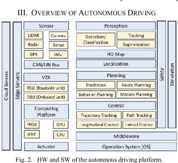
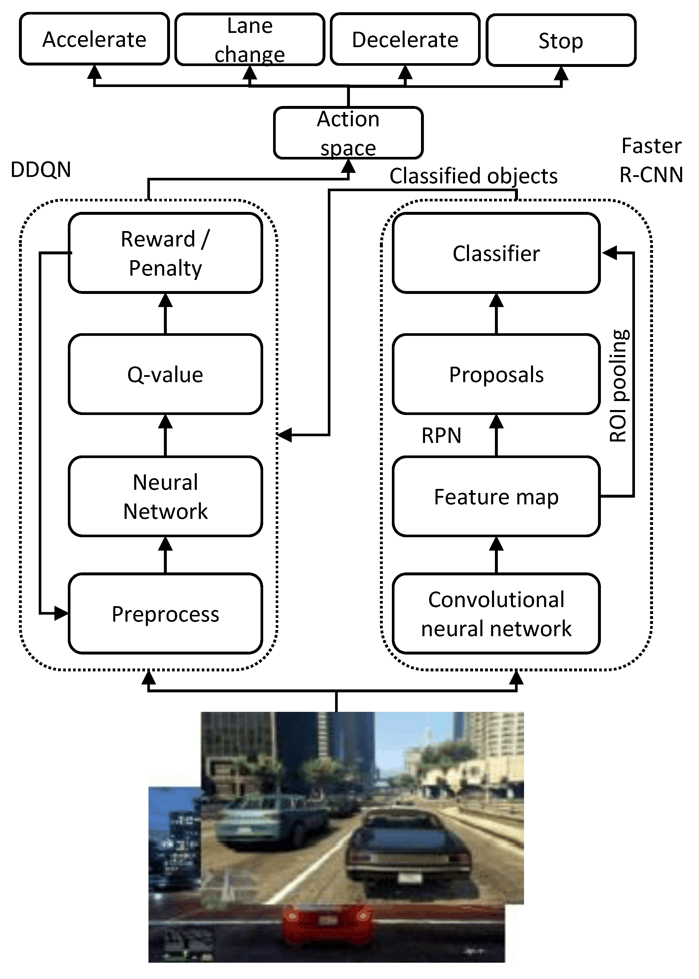
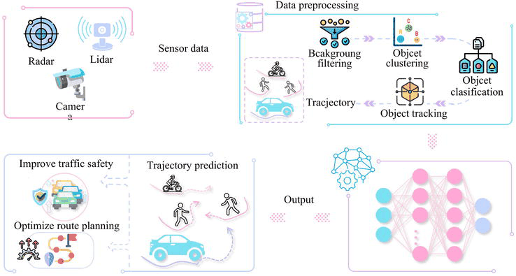
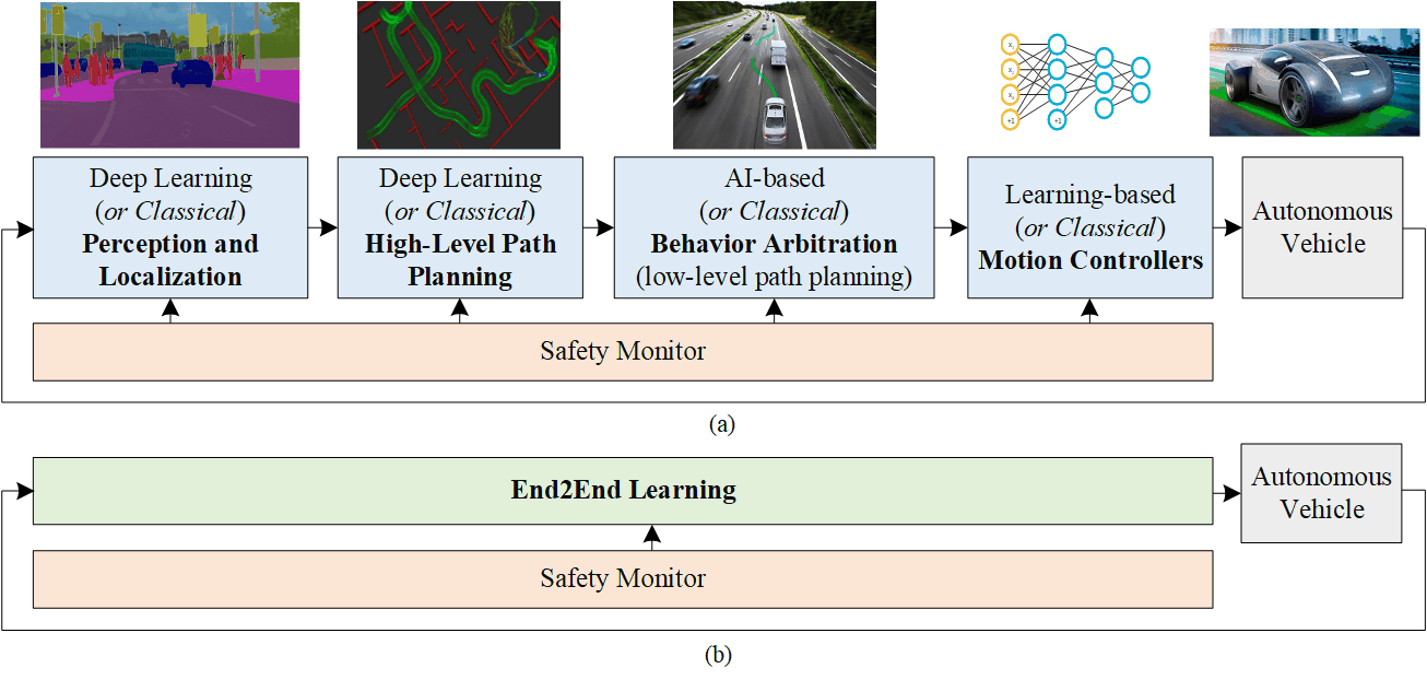
Deep Learning Execution Pipeline
(Preprocessing)
(Feature Extraction)
(Self-Attention)
(Loss Optimization)