Complete Technical Paper Content — Clustering Algorithms Projects
1. Executive Abstract, Problem Formulation & Background
The following outline is provided as an overview of, and topical guide to, machine learning: Machine learning (ML) is a subfield of artificial intelligence within computer science that evolved from the study of pattern recognition and computational learning theory. In 1959, Arthur Samuel defined machine learning as a "field of study that gives computers the ability to learn without being explicitly programmed". ML involves the study and construction of algorithms that can learn from and make predictions on data. These algorithms operate by building a model from a training set of example observations to make data-driven predictions or decisions expressed as outputs, rather than following strictly static program instructions.
Canonical correlation analysis (CCA) Factor analysis Feature extraction Feature selection Independent component analysis (ICA) Linear discriminant analysis (LDA) Multidimensional scaling (MDS) Non-negative matrix factorization (NMF) Partial least squares regression (PLSR) Principal component analysis (PCA) Principal component regression (PCR) Projection pursuit Sammon mapping t-distributed stochastic neighbor embedding (t-SNE)
AdaBoost Boosting Bootstrap aggregating (also "bagging" or "bootstrapping") Ensemble averaging Gradient boosted decision tree (GBDT) Gradient boosting Random Forest Stacked Generalization
Q-learning State–action–reward–state–action (SARSA) Temporal difference learning (TD) Learning Automata
Averaged one-dependence estimators (AODE) Artificial neural network Case-based reasoning Gaussian process regression Gene expression programming Group method of data handling (GMDH) Inductive logic programming Instance-based learning Lazy learning Learning Automata Learning Vector Quantization Logistic Model Tree Minimum message length (decision trees, decision graphs, etc.) Nearest Neighbor Algorithm Analogical modeling Probably approximately correct learning (PAC) learning Ripple down rules, a knowledge acquisition methodology Symbolic machine learning algorithms Support vector machines Random Forests Ensembles of classifiers Bootstrap aggregating (bagging) Boosting (meta-algorithm) Ordinal classification Conditional Random Field ANOVA Quadratic classifiers k-nearest neighbor Boosting SPRINT Bayesian networks Naive Bayes Hidden Markov models Hierarchical hidden Markov model
Bayesian knowledge base Naive Bayes Gaussian Naive Bayes Multinomial Naive Bayes Averaged One-Dependence Estimators (AODE) Bayesian Belief Network (BBN) Bayesian Network (BN)
Decision tree Classification and regression tree (CART) Iterative Dichotomiser 3 (ID3) C4.5 algorithm C5.0 algorithm Chi-squared Automatic Interaction Detection (CHAID) Decision stump Conditional decision tree ID3 algorithm Random forest SLIQ
Fisher's linear discriminant Linear regression Logistic regression Multinomial logistic regression Naive Bayes classifier Perceptron Support vector machine
Expectation-maximization algorithm Vector Quantization Generative topographic map Information bottleneck method Association rule learning algorithms Apriori algorithm Eclat algorithm
2. Related Work, Literature Survey & Algorithmic Foundations
Feedforward neural network Extreme learning machine Convolutional neural network Recurrent neural network Long short-term memory (LSTM) Logic learning machine Self-organizing map
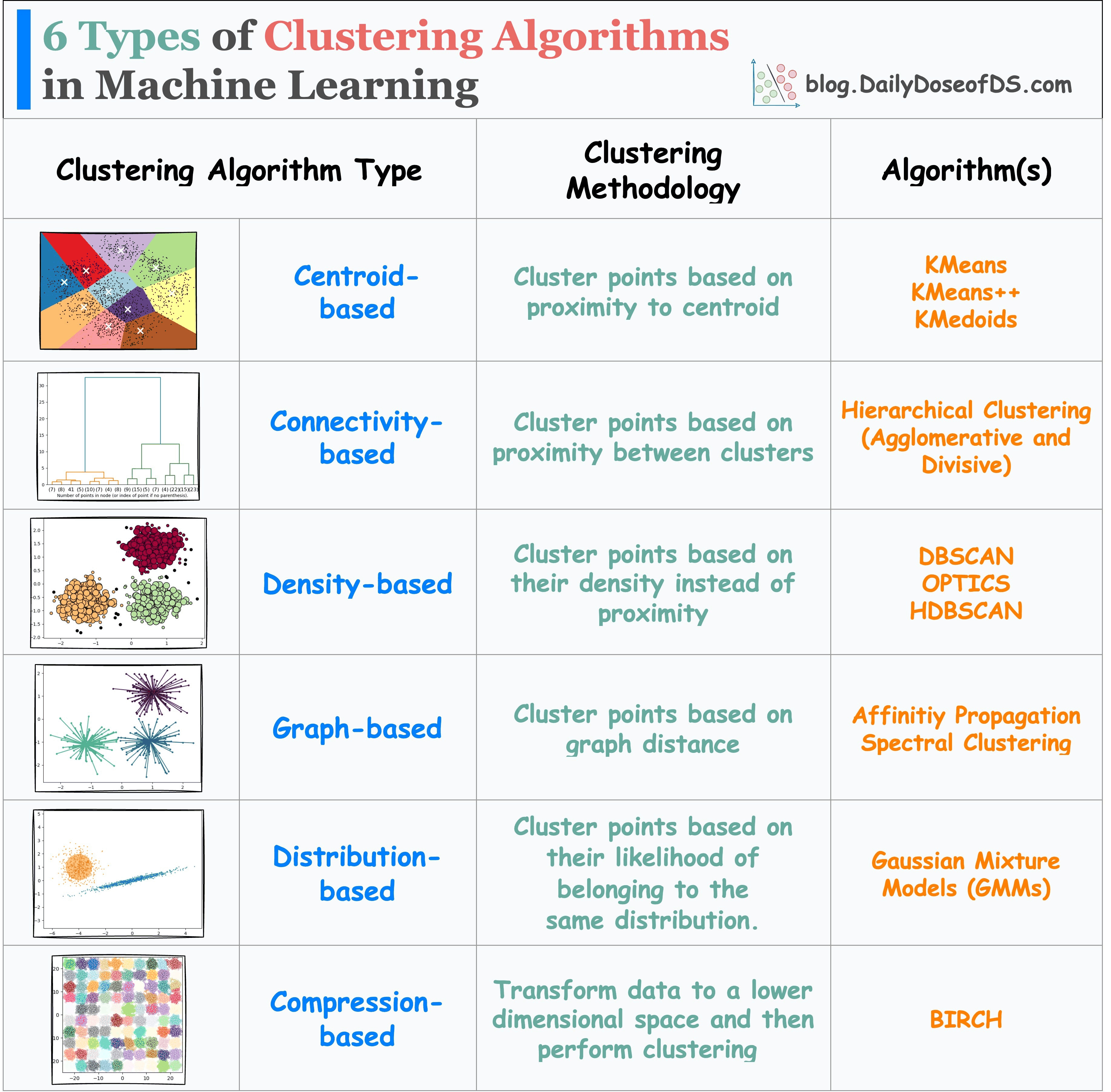
BIRCH DBSCAN Expectation–maximization (EM) Fuzzy clustering Hierarchical clustering k-means clustering k-medians Mean-shift OPTICS algorithm
Active learning Generative models Low-density separation Graph-based methods Co-training Transduction
Deep belief networks Deep Boltzmann machines Deep Convolutional neural networks Deep Recurrent neural networks Hierarchical temporal memory Generative Adversarial Network Style transfer Transformer Stacked Auto-Encoders
Data Science: Data to Insights from MIT (machine learning) Popular online course by Andrew Ng, at Coursera. It uses GNU Octave. The course is a free version of Stanford University's actual course taught by Ng, see.stanford.edu/Course/CS229 available for free]. mloss is an academic database of open-source machine learning software.
k-means clustering is a method of vector quantization, originally from signal processing, that aims to partition n observations into k clusters in which each observation belongs to the cluster with the nearest mean (cluster centers or cluster centroid). This results in a partitioning of the data space into Voronoi cells. k-means clustering minimizes within-cluster variances (squared Euclidean distances), but not regular Euclidean distances, which would be the more difficult Weber problem: the mean optimizes squared errors, whereas only the geometric median minimizes Euclidean distances. For instance, better Euclidean solutions can be found using k-medians and k-medoids. The problem is computationally difficult (NP-hard); however, efficient heuristic algorithms converge quickly to a local optimum. These are usually similar to the expectation–maximization algorithm for mixtures of Gaussian distributions via an iterative refinement approach employed by both k-means and Gaussian mixture modeling. They both use cluster centers to model the data; however, k-means clustering tends to find clusters of comparable spatial extent, while the Gaussian mixture model allows clusters to have different shapes. The unsupervised k-means algorithm has a loose relationship to the k-nearest neighbor classifier, a popular supervised machine learning technique for classification that is often confused with k-means due to the name. Applying the 1-nearest neighbor classifier to the cluster centers obtained by k-means classifies new data into the existing clusters. This is known as nearest centroid classifier or Rocchio algorithm.
a r g m i n S ∑ i = 1 k ∑ x ∈ S i ‖ x − μ i ‖ 2 = a r g m i n S ∑ i = 1 k | S i | Var S i {\displaystyle \mathop {\operatorname {arg\,min} } _{\mathbf {S} }\sum _{i=1}^{k}\sum _{\mathbf {x} \in S_{i}}\left\|\mathbf {x} -{\boldsymbol {\mu }}_{i}\right\|^{2}=\mathop {\operatorname {arg\,min} } _{\mathbf {S} }\sum _{i=1}^{k}|S_{i}|\operatorname {Var} S_{i}}
where μi is the mean (also called centroid) of points in S i {\displaystyle S_{i}} , i.e.
μ i = 1 | S i | ∑ x ∈ S i x , {\displaystyle {\boldsymbol {\mu _{i}}}={\frac {1}{|S_{i}|}}\sum _{\mathbf {x} \in S_{i}}\mathbf {x} ,}
3. Dataset Ingestion, Preprocessing & Stochastic Augmentations
| S i | {\displaystyle |S_{i}|} is the size of S i {\displaystyle S_{i}} , and ‖ ⋅ ‖ {\displaystyle \|\cdot \|} is the usual L2 norm . This is equivalent to minimizing the pairwise squared deviations of points in the same cluster:
a r g m i n S ∑ i = 1 k 1 | S i | ∑ x , y ∈ S i ‖ x − y ‖ 2 {\displaystyle \mathop {\operatorname {arg\,min} } _{\mathbf {S} }\sum _{i=1}^{k}\,{\frac {1}{|S_{i}|}}\,\sum _{\mathbf {x} ,\mathbf {y} \in S_{i}}\left\|\mathbf {x} -\mathbf {y} \right\|^{2}}
The equivalence can be deduced from the identity | S i | ∑ x ∈ S i ‖ x − μ i ‖ 2 = 1 2 ∑ x , y ∈ S i ‖ x − y ‖ 2 {\textstyle |S_{i}|\sum _{\mathbf {x} \in S_{i}}\left\|\mathbf {x} -{\boldsymbol {\mu }}_{i}\right\|^{2}={\frac {1}{2}}\sum _{\mathbf {x} ,\mathbf {y} \in S_{i}}\left\|\mathbf {x} -\mathbf {y} \right\|^{2}} . Since the total variance is constant, this is equivalent to maximizing the sum of squared deviations between points in different clusters (between-cluster sum of squares, BCSS). This deterministic relationship is also related to the law of total variance in probability theory.
Early applications of the k-means algorithm were primarily found in signal processing and data compression, particularly in the context of vector quantization. Lloyd's work at Bell Labs focused on representing analog signals using a limited set of discrete values, where clustering was used to reduce the amount of data required while preserving signal quality. As computing power increased, k-means clustering became widely used in pattern recognition and statistical classification due to its simplicity and computational efficiency. It was later adopted in early machine learning and data analysis tasks involving large datasets. Despite its widespread use, limitations such as sensitivity to initial centroid placement and difficulty handling non-spherical clusters were recognized early on, motivating the development of improved clustering methods and initialization techniques. Numerous extensions of k-means have since been developed to address limitations of the original algorithm, including methods such as fuzzy c-means, which allows data points to belong to multiple clusters with varying degrees of membership, and kernel k-means, which uses kernel functions to identify non-linearly separable clusters.
The most common algorithm uses an iterative refinement technique. Due to its ubiquity, it is often called "the k-means algorithm"; it is also referred to as Lloyd's algorithm, particularly in the computer science community. It is sometimes also referred to as "naïve k-means", because there exist much faster alternatives. Given an initial set of k means m1(1), ..., mk(1) (see below), the algorithm proceeds by alternating between two steps:
Assignment step: Assign each observation to the cluster with the nearest mean (centroid): that with the least squared Euclidean distance. (Mathematically, this means partitioning the observations according to the Voronoi diagram generated by the means.) S i ( t ) = { x p : ‖ x p − m i ( t ) ‖ 2 ≤ ‖ x p − m j ( t ) ‖ 2 ∀ j , 1 ≤ j ≤ k } , {\displaystyle S_{i}^{(t)}=\left\{x_{p}:\left\|x_{p}-m_{i}^{(t)}\right\|^{2}\leq \left\|x_{p}-m_{j}^{(t)}\right\|^{2}\ \forall j,1\leq j\leq k\right\},} where each x p {\displaystyle x_{p}} is assigned to exactly one S ( t ) {\displaystyle S^{(t)}} , even if it could be assigned to two or more of them. Update step: Recalculate means (centroids) for observations assigned to each cluster. This is also called refitting. m i ( t + 1 ) = 1 | S i ( t ) | ∑ x j ∈ S i ( t ) x j {\displaystyle m_{i}^{(t+1)}={\frac {1}{\left|S_{i}^{(t)}\right|}}\sum _{x_{j}\in S_{i}^{(t)}}x_{j}}
The objective function in k-means is the WCSS (within cluster sum of squares). After each iteration, the WCSS monotonically decreases, giving a nonnegative monotonically decreasing sequence. This guarantees that the k-means always converges, but not necessarily to the global optimum. The algorithm has converged when the assignments no longer change or equivalently, when the WCSS has become stable. The algorithm is not guaranteed to find the optimal cluster assignment. The algorithm is often presented as assigning objects to the nearest cluster by distance. Using a different distance function other than (squared) Euclidean distance may prevent the algorithm from converging. Various modifications of k-means such as spherical k-means and k-medoids have been proposed to allow using other distance measures.
Pseudocode The below pseudocode outlines the implementation of the standard k-means clustering algorithm. Initialization of centroids, distance metric between points and centroids, and the calculation of new centroids are design choices and will vary with different implementations. In this example pseudocode, distance() returns the distance between the specified points.
function kmeans(k, points) is // Initialize centroids centroids ← list of k starting centroids converged ← false
4. Neural Network Backbone, Layer Specifications & Loss Formulations
while converged == false do // Create empty clusters clusters ← list of k empty lists
// Assign each point to the nearest centroid for i ← 0 to length(points) - 1 do point ← points[i] closestIndex ← 0 minDistance ← distance(point, centroids[0]) for j ← 1 to k - 1 do d ← distance(point, centroids[j]) if d < minDistance THEN minDistance ← d closestIndex ← j clusters[closestIndex].append(point)
// Recalculate centroids as the mean of each cluster newCentroids ← empty list for i ← 0 to k - 1 do newCentroid ← calculateCentroid(clusters[i]) newCentroids.append(newCentroid)
// Check for convergence if newCentroids == centroids THEN converged ← true else centroids ← newCentroids
The algorithm does not guarantee convergence to the global optimum. The result may depend on the initial clusters. As the algorithm is usually fast, it is common to run it multiple times with different starting conditions. However, worst-case performance can be slow: in particular certain point sets, even in two dimensions, converge in exponential time, that is 2Ω(n). These point sets do not seem to arise in practice: this is corroborated by the fact that the smoothed running time of k-means is polynomial. The "assignment" step is referred to as the "expectation step", while the "update step" is a maximization step, making this algorithm a variant of the generalized expectation–maximization algorithm.
NP-hard in general Euclidean space (of d dimensions) even for two clusters, NP-hard for a general number of clusters k even in the plane, if k and d (the dimension) are fixed, the problem can be exactly solved in time O ( n d k + 1 ) {\displaystyle O(n^{dk+1})} , where n is the number of entities to be clustered. Thus, a variety of heuristic algorithms such as Lloyd's algorithm given above are generally used. The running time of Lloyd's algorithm (and most variants) is O ( n k d i ) {\displaystyle O(nkdi)} , where:
n is the number of d-dimensional vectors (to be clustered) k the number of clusters i the number of iterations needed until convergence. On data that does have a clustering structure, the number of iterations until convergence is often small, and results only improve slightly after the first dozen iterations. Lloyd's algorithm is therefore often considered to be of "linear" complexity in practice, although it is in the worst case superpolynomial when performed until convergence.
In the worst-case, Lloyd's algorithm needs i = 2 Ω ( n ) {\displaystyle i=2^{\Omega ({\sqrt {n}})}} iterations, so that the worst-case complexity of Lloyd's algorithm is superpolynomial. Lloyd's k-means algorithm has polynomial smoothed running time. It is shown that for arbitrary set of n points in [ 0 , 1 ] d {\displaystyle [0,1]^{d}} , if each point is independently perturbed by a normal distribution with mean 0 and variance σ 2 {\displaystyle \sigma ^{2}} , then the expected running time of k-means algorithm is bounded by O ( n 34 k 34 d 8 log 4 ( n ) / σ 6 ) {\displaystyle O(n^{34}k^{34}d^{8}\log ^{4}(n)/\sigma ^{6})} , which is a polynomial in n, k, d and 1 / σ {\displaystyle 1/\sigma } . Better bounds are proven for simple cases. For example, it is shown that the running time of k-means algorithm is bounded by O ( d n 4 M 2 ) {\displaystyle O(dn^{4}M^{2})} for n points in an integer lattice { 1 , … , M } d {\displaystyle \{1,\dots ,M\}^{d}} . Lloyd's algorithm is the standard approach for this problem. However, it spends a lot of processing time computing the distances between each of the k cluster centers and the n data points. Since points usually stay in the same clusters after a few iterations, much of this work is unnecessary, making the naïve implementation very inefficient. Some implementations use caching and the triangle inequality in order to create bounds and accelerate Lloyd's algorithm.
Finding the optimal number of clusters (k) for k-means clustering is a crucial step to ensure that the clustering results are meaningful and useful. Several techniques are available to determine a suitable number of clusters. Here are some of commonly used methods:
5. Training Protocol, Convergence Behavior & Experimental Evaluation
Elbow method (clustering): This method involves plotting the explained variation as a function of the number of clusters, and picking the elbow of the curve as the number of clusters to use. However, the notion of an "elbow" is not well-defined and this is known to be unreliable. Silhouette (clustering): Silhouette analysis measures the quality of clustering and provides an insight into the separation distance between the resulting clusters. A higher silhouette score indicates that the object is well matched to its own cluster and poorly matched to neighboring clusters. Gap statistic: The Gap Statistic compares the total within intra-cluster variation for different values of k with their expected values under null reference distribution of the data. The optimal k is the value that yields the largest gap statistic. Davies–Bouldin index: The Davies-Bouldin index is a measure of the how much separation there is between clusters. Lower values of the Davies-Bouldin index indicate a model with better separation. Calinski-Harabasz index: This Index evaluates clusters based on their compactness and separation. The index is calculated using the ratio of between-cluster variance to within-cluster variance, with higher values indicate better-defined clusters. Rand index: It calculates the proportion of agreement between the two clusters, considering both the pairs of elements that are correctly assigned to the same or different clusters. Higher values indicate greater similarity and better clustering quality. To provide a more accurate measure, the Adjusted Rand Index (ARI), introduced by Hubert and Arabie in 1985, corrects the Rand Index by adjusting for the expected similarity of all pairings due to chance.
Assignment step Hartigan and Wong's method starts by partitioning the points into random clusters { S j } j ∈ { 1 , ⋯ k } {\displaystyle \{S_{j}\}_{j\in \{1,\cdots k\}}} . Update step Next it determines the n , m ∈ { 1 , … , k } {\displaystyle n,m\in \{1,\ldots ,k\}} and x ∈ S n {\displaystyle x\in S_{n}} for which the following function reaches a maximum Δ ( m , n , x ) = φ ( S n ) + φ ( S m ) − φ ( S n ∖ { x } ) − φ ( S m ∪ { x } ) . {\displaystyle \Delta (m,n,x)=\varphi (S_{n})+\varphi (S_{m})-\varphi (S_{n}\setminus \{x\})-\varphi (S_{m}\cup \{x\}).} For the x , n , m {\displaystyle x,n,m} that reach this maximum, x {\displaystyle x} moves from the cluster S n {\displaystyle S_{n}} to the cluster S m {\displaystyle S_{m}} . Termination The algorithm terminates once Δ ( m , n , x ) {\displaystyle \Delta (m,n,x)} is less than zero for all x , n , m {\displaystyle x,n,m} . Different move acceptance strategies can be used. In a first-improvement strategy, any improving relocation can be applied, whereas in a best-improvement strategy, all possible relocations are iteratively tested and only the best is applied at each iteration. The former approach favors speed, whether the latter approach generally favors solution quality at the expense of additional computational time. The function Δ {\displaystyle \Delta } used to calculate the result of a relocation can also be efficiently evaluated by using equality
Δ ( x , n , m ) = ∣ S n ∣ ∣ S n ∣ − 1 ⋅ ‖ μ n − x ‖ 2 − ∣ S m ∣ ∣ S m ∣ + 1 ⋅ ‖ μ m − x ‖ 2 . {\displaystyle \Delta (x,n,m)={\frac {\mid S_{n}\mid }{\mid S_{n}\mid -1}}\cdot \lVert \mu _{n}-x\rVert ^{2}-{\frac {\mid S_{m}\mid }{\mid S_{m}\mid +1}}\cdot \lVert \mu _{m}-x\rVert ^{2}.}
a r g m i n S ∑ i = 1 k ∑ x ∈ S i ‖ x − μ i ‖ 2 . {\displaystyle \mathop {\operatorname {arg\,min} } _{\mathbf {S} }\sum _{i=1}^{k}\sum _{\mathbf {x} \in S_{i}}\left\|\mathbf {x} -{\boldsymbol {\mu }}_{i}\right\|^{2}.}
Many studies have attempted to improve the convergence behavior of the algorithm and maximize the chances of attaining the global optimum (or at least, local minima of better quality). Initialization and restart techniques discussed in the previous sections are one alternative to find better solutions. More recently, global optimization algorithms based on branch-and-bound and semidefinite programming have produced provenly optimal solutions for datasets with up to 4,177 entities and 20,531 features. As expected, due to the NP-hardness of the subjacent optimization problem, the computational time of optimal algorithms for k-means quickly increases beyond this size. Optimal solutions for small- and medium-scale still remain valuable as a benchmark tool, to evaluate the quality of other heuristics. To find high-quality local minima within a controlled computational time but without optimality guarantees, other works have explored metaheuristics and other global optimization techniques, e.g., based on incremental approaches and convex optimization, random swaps (i.e., iterated local search), variable neighborhood search and genetic algorithms. It is indeed known that finding better local minima of the minimum sum-of-squares clustering problem can make the difference between failure and success to recover cluster structures in feature spaces of high dimension.
Three key features of k-means that make it efficient are often regarded as its biggest drawbacks:
Euclidean distance is used as a metric and variance is used as a measure of cluster scatter. The number of clusters k is an input parameter: an inappropriate choice of k may yield poor results. That is why, when performing k-means, it is important to run diagnostic checks for determining the number of clusters in the data set. Convergence to a local minimum may produce counterintuitive ("wrong") results (see example in Fig.). A key limitation of k-means is its cluster model. The concept is based on spherical clusters that are separable so that the mean converges towards the cluster center. The clusters are expected to be of similar size, so that the assignment to the nearest cluster center is the correct assignment. When for example applying k-means with a value of k = 3 {\displaystyle k=3} onto the well-known Iris flower data set, the result often fails to separate the three Iris species contained in the data set. With k = 2 {\displaystyle k=2} , the two visible clusters (one containing two species) will be discovered, whereas with k = 3 {\displaystyle k=3} one of the two clusters will be split into two even parts. In fact, k = 2 {\displaystyle k=2} is more appropriate for this data set, despite the data set's containing 3 classes. As with any other clustering algorithm, the k-means result makes assumptions that the data satisfy certain criteria. It works well on some data sets, and fails on others. The result of k-means can be seen as the Voronoi cells of the cluster means. Since data is split halfway between cluster means, this can lead to suboptimal splits as can be seen in the "mouse" example. The Gaussian models used by the expectation–maximization algorithm (arguably a generalization of k-means) are more flexible by having both variances and covariances. The EM result is thus able to accommodate clusters of variable size much better than k-means as well as correlated clusters (not in this example). In counterpart, EM requires the optimization of a larger number of free parameters and poses some methodological issues due to vanishing clusters or badly-conditioned covariance matrices. k-means is closely related to nonparametric Bayesian modeling.
In biological applications, the limitations of standard k-means clustering are often addressed by adapting the distance measures used and objective functions to better reflect the structure of experimental data. Rather than relying on Euclidean distance and variance-based measures of cluster scatter, alternative similarity metrics such as the Jaccard index are sometimes used when analyzing genomic datasets with k-means. In these contexts, clustering may be performed directly on distance matrices, and medoids (representative data points that have the smallest average distance to every other point within a cluster) may be selected as cluster centers instead of arithmetic means. This allows clustering methods to capture patterns of shared genomic features or co-occurrence that are not well represented in a traditional Euclidean analysis. Clustering is widely used in biological data analysis to identify patterns in high-dimensional datasets such as gene expression profiles and genomic interaction matrices. Techniques such as k-means clustering partition observations into groups based on similarity, allowing researchers to detect structure in complex datasets. In gene expression studies, clustering is commonly used to group genes with similar expression profiles, often revealing co-regulated genes and underlying biological interactions. In addition to gene expression analysis, clustering approaches are applied to chromatin interaction data to identify regions of coordinated activity. Similarity measures such as the Jaccard index can be used to quantify shared features between observations, and clustering of the resulting distance matrices can reveal structural organization within the genome. These patterns are commonly visualized using heatmaps, where clustered regions correspond to domains of interaction or co-segregation, providing insight into the regulatory organization of the genome. In such analyses, clustering of similarity or co-detection matrices can reveal groups of genomic windows that exhibit coordinated behavior across experimental conditions. Clustering methods provide a practical method for uncovering biologically meaningful structure from complex datasets. By grouping observations with similar patterns of genomic detection, expression, or interaction, these techniques can reveal functional relationships, spatial organization within the nucleus, and regulatory behavior. In many applications, the resulting clusters correspond to distinct biological states or structural domains, further illustrating the broad applicability of k-means clustering.
Vector quantization, a technique commonly used in signal processing and computer graphics, involves reducing the color palette of an image to a fixed number of colors, known as k. One popular method for achieving vector quantization is through k-means clustering. In this process, k-means is applied to the color space of an image to partition it into k clusters, with each cluster representing a distinct color in the image. This technique is particularly useful in image segmentation tasks, where it helps identify and group similar colors together.
Model Figures & Evaluation Curves (4 Images)
Deep Learning Execution Pipeline
(Preprocessing)
(Feature Extraction)
(Self-Attention)
(Loss Optimization)