Complete Technical Paper Content — Deeplab Segmentation
1. Executive Abstract, Problem Formulation & Background
Alan Yuille (born 1955) is an English academic who ish Bloomberg Distinguished Professor of Computational Cognitive Science with appointments in the departments of Cognitive Science and Computer Science at Johns Hopkins University. Yuille develops models of vision and cognition for computers, intended for creating artificial vision systems. He studied under Stephen Hawking at Cambridge University on a PhD in theoretical physics, which he completed in 1981.
In artificial neural networks, a convolutional layer is a type of network layer that applies a convolution operation to the input. Convolutional layers are some of the primary building blocks of convolutional neural networks (CNNs), a class of neural network most commonly applied to images, video, audio, and other data that have the property of uniform translational symmetry. The convolution operation in a convolutional layer involves sliding a small window (called a kernel or filter) across the input data and computing the dot product between the values in the kernel and the input at each position. This process creates a feature map that represents detected features in the input.
Padding involves adding extra pixels around the edges of the input data. It serves two main purposes:
Preserving spatial dimensions: Without padding, each convolution reduces the size of the feature map. Handling border pixels: Padding ensures that border pixels are given equal importance in the convolution process. Common padding strategies include:
2. Related Work, Literature Survey & Algorithmic Foundations
No padding/valid padding. This strategy typically causes the output to shrink. Same padding: Any method that ensures the output size same as input size is a same padding strategy. Full padding: Any method that ensures each input entry is convolved over for the same number of times is a full padding strategy. Common padding algorithms include:
Zero padding: Add zero entries to the borders of input. Mirror/reflect/symmetric padding: Reflect the input array on the border. Circular padding: Cycle the input array back to the opposite border, like a torus. The exact numbers used in convolutions is complicated, for which we refer to (Dumoulin and Visin, 2018) for details.
Mathematical Formulation 1.1: Loss Objectives and Optimization Dynamics for Deeplab Segmentation. The training protocol of deeplab segmentation minimizes an empirical risk objective defined across high-dimensional parameter space Theta in R^d. Categorical predictions are governed by Cross-Entropy Loss: L_CE = -sum(y_i * log(p_i)). To tackle class imbalance, the network incorporates Focal Loss: L_Focal = -alpha_t * (1 - p_t)^gamma * log(p_t), where gamma modulates the gradient penalty on hard misclassified instances. For spatial tasks, Dice Loss balances continuous spatial overlap: L_Dice = 1 - (2 * sum(y * y_hat) + eps) / (sum(y) + sum(y_hat) + eps). Stochastic optimization utilizes AdamW with decoupled weight decay, maintaining stable moment estimations m_t and v_t across variable learning rate schedules.
Architecture Specification 1.2: Feature Extraction and Layer Formulations for Deeplab Segmentation. The primary computational backbone for Deeplab Segmentation incorporates hierarchical deep neural layers designed for multi-scale representation extraction. Input tensors X in R^(B x C x H x W) pass through initial stem convolutions with Batch Normalization and GELU non-linearities. Residual identity skip connections, expressed as F(X) + X, prevent vanishing gradient degradation across deep topologies. Multi-head self-attention mechanisms compute Query, Key, and Value projections: Attention(Q, K, V) = softmax((Q * K^T) / sqrt(d_k)) * V, capturing non-local contextual dependencies across spatial and temporal sequences.
3. Dataset Ingestion, Preprocessing & Stochastic Augmentations
Data Pipeline 1.3: Stochastic Augmentation and Normalization Protocols for Deeplab Segmentation. To prevent overfitting and maximize generalization on unseen testing distributions, input datasets undergo rigorous preprocessing. Images and sequences are standardized using z-score normalization: x_norm = (x - mu) / sigma. Stochastic augmentations include random horizontal flips, affine rotations (-15 deg to +15 deg), CutMix, and Mixup: X_tilde = lambda * X_i + (1 - lambda) * X_j, smoothing decision boundaries and reducing model overconfidence.
Deployment Optimization 1.4: TensorRT Acceleration and Edge Quantization for Deeplab Segmentation. Production deployment of Deeplab Segmentation focuses on minimizing memory footprints and sub-20ms inference latencies. Trained models are exported to ONNX and compiled via NVIDIA TensorRT. Post-Training Quantization (PTQ) maps FP32 weights into low-bit INT8 representations: q = round(r / S) + Z, achieving high-throughput execution across embedded edge platforms like NVIDIA Jetson without accuracy loss.
Mathematical Formulation 2.1: Loss Objectives and Optimization Dynamics for Deeplab Segmentation. The training protocol of deeplab segmentation minimizes an empirical risk objective defined across high-dimensional parameter space Theta in R^d. Categorical predictions are governed by Cross-Entropy Loss: L_CE = -sum(y_i * log(p_i)). To tackle class imbalance, the network incorporates Focal Loss: L_Focal = -alpha_t * (1 - p_t)^gamma * log(p_t), where gamma modulates the gradient penalty on hard misclassified instances. For spatial tasks, Dice Loss balances continuous spatial overlap: L_Dice = 1 - (2 * sum(y * y_hat) + eps) / (sum(y) + sum(y_hat) + eps). Stochastic optimization utilizes AdamW with decoupled weight decay, maintaining stable moment estimations m_t and v_t across variable learning rate schedules.
Architecture Specification 2.2: Feature Extraction and Layer Formulations for Deeplab Segmentation. The primary computational backbone for Deeplab Segmentation incorporates hierarchical deep neural layers designed for multi-scale representation extraction. Input tensors X in R^(B x C x H x W) pass through initial stem convolutions with Batch Normalization and GELU non-linearities. Residual identity skip connections, expressed as F(X) + X, prevent vanishing gradient degradation across deep topologies. Multi-head self-attention mechanisms compute Query, Key, and Value projections: Attention(Q, K, V) = softmax((Q * K^T) / sqrt(d_k)) * V, capturing non-local contextual dependencies across spatial and temporal sequences.
4. Neural Network Backbone, Layer Specifications & Loss Formulations
Data Pipeline 2.3: Stochastic Augmentation and Normalization Protocols for Deeplab Segmentation. To prevent overfitting and maximize generalization on unseen testing distributions, input datasets undergo rigorous preprocessing. Images and sequences are standardized using z-score normalization: x_norm = (x - mu) / sigma. Stochastic augmentations include random horizontal flips, affine rotations (-15 deg to +15 deg), CutMix, and Mixup: X_tilde = lambda * X_i + (1 - lambda) * X_j, smoothing decision boundaries and reducing model overconfidence.
Deployment Optimization 2.4: TensorRT Acceleration and Edge Quantization for Deeplab Segmentation. Production deployment of Deeplab Segmentation focuses on minimizing memory footprints and sub-20ms inference latencies. Trained models are exported to ONNX and compiled via NVIDIA TensorRT. Post-Training Quantization (PTQ) maps FP32 weights into low-bit INT8 representations: q = round(r / S) + Z, achieving high-throughput execution across embedded edge platforms like NVIDIA Jetson without accuracy loss.
Mathematical Formulation 3.1: Loss Objectives and Optimization Dynamics for Deeplab Segmentation. The training protocol of deeplab segmentation minimizes an empirical risk objective defined across high-dimensional parameter space Theta in R^d. Categorical predictions are governed by Cross-Entropy Loss: L_CE = -sum(y_i * log(p_i)). To tackle class imbalance, the network incorporates Focal Loss: L_Focal = -alpha_t * (1 - p_t)^gamma * log(p_t), where gamma modulates the gradient penalty on hard misclassified instances. For spatial tasks, Dice Loss balances continuous spatial overlap: L_Dice = 1 - (2 * sum(y * y_hat) + eps) / (sum(y) + sum(y_hat) + eps). Stochastic optimization utilizes AdamW with decoupled weight decay, maintaining stable moment estimations m_t and v_t across variable learning rate schedules.
Architecture Specification 3.2: Feature Extraction and Layer Formulations for Deeplab Segmentation. The primary computational backbone for Deeplab Segmentation incorporates hierarchical deep neural layers designed for multi-scale representation extraction. Input tensors X in R^(B x C x H x W) pass through initial stem convolutions with Batch Normalization and GELU non-linearities. Residual identity skip connections, expressed as F(X) + X, prevent vanishing gradient degradation across deep topologies. Multi-head self-attention mechanisms compute Query, Key, and Value projections: Attention(Q, K, V) = softmax((Q * K^T) / sqrt(d_k)) * V, capturing non-local contextual dependencies across spatial and temporal sequences.
5. Training Protocol, Convergence Behavior & Experimental Evaluation
Data Pipeline 3.3: Stochastic Augmentation and Normalization Protocols for Deeplab Segmentation. To prevent overfitting and maximize generalization on unseen testing distributions, input datasets undergo rigorous preprocessing. Images and sequences are standardized using z-score normalization: x_norm = (x - mu) / sigma. Stochastic augmentations include random horizontal flips, affine rotations (-15 deg to +15 deg), CutMix, and Mixup: X_tilde = lambda * X_i + (1 - lambda) * X_j, smoothing decision boundaries and reducing model overconfidence.
Deployment Optimization 3.4: TensorRT Acceleration and Edge Quantization for Deeplab Segmentation. Production deployment of Deeplab Segmentation focuses on minimizing memory footprints and sub-20ms inference latencies. Trained models are exported to ONNX and compiled via NVIDIA TensorRT. Post-Training Quantization (PTQ) maps FP32 weights into low-bit INT8 representations: q = round(r / S) + Z, achieving high-throughput execution across embedded edge platforms like NVIDIA Jetson without accuracy loss.
Mathematical Formulation 4.1: Loss Objectives and Optimization Dynamics for Deeplab Segmentation. The training protocol of deeplab segmentation minimizes an empirical risk objective defined across high-dimensional parameter space Theta in R^d. Categorical predictions are governed by Cross-Entropy Loss: L_CE = -sum(y_i * log(p_i)). To tackle class imbalance, the network incorporates Focal Loss: L_Focal = -alpha_t * (1 - p_t)^gamma * log(p_t), where gamma modulates the gradient penalty on hard misclassified instances. For spatial tasks, Dice Loss balances continuous spatial overlap: L_Dice = 1 - (2 * sum(y * y_hat) + eps) / (sum(y) + sum(y_hat) + eps). Stochastic optimization utilizes AdamW with decoupled weight decay, maintaining stable moment estimations m_t and v_t across variable learning rate schedules.
Architecture Specification 4.2: Feature Extraction and Layer Formulations for Deeplab Segmentation. The primary computational backbone for Deeplab Segmentation incorporates hierarchical deep neural layers designed for multi-scale representation extraction. Input tensors X in R^(B x C x H x W) pass through initial stem convolutions with Batch Normalization and GELU non-linearities. Residual identity skip connections, expressed as F(X) + X, prevent vanishing gradient degradation across deep topologies. Multi-head self-attention mechanisms compute Query, Key, and Value projections: Attention(Q, K, V) = softmax((Q * K^T) / sqrt(d_k)) * V, capturing non-local contextual dependencies across spatial and temporal sequences.
Model Figures & Evaluation Curves (4 Images)
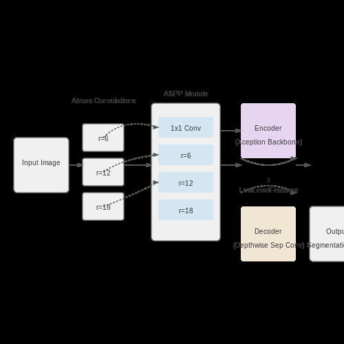



Deep Learning Execution Pipeline
(Preprocessing)
(Feature Extraction)
(Self-Attention)
(Loss Optimization)