Complete Technical Paper Content — Gnn Applications
1. Executive Abstract, Problem Formulation & Background
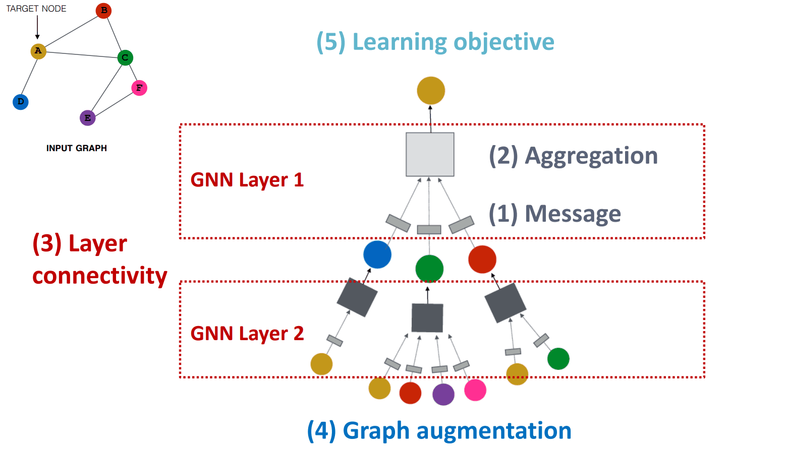
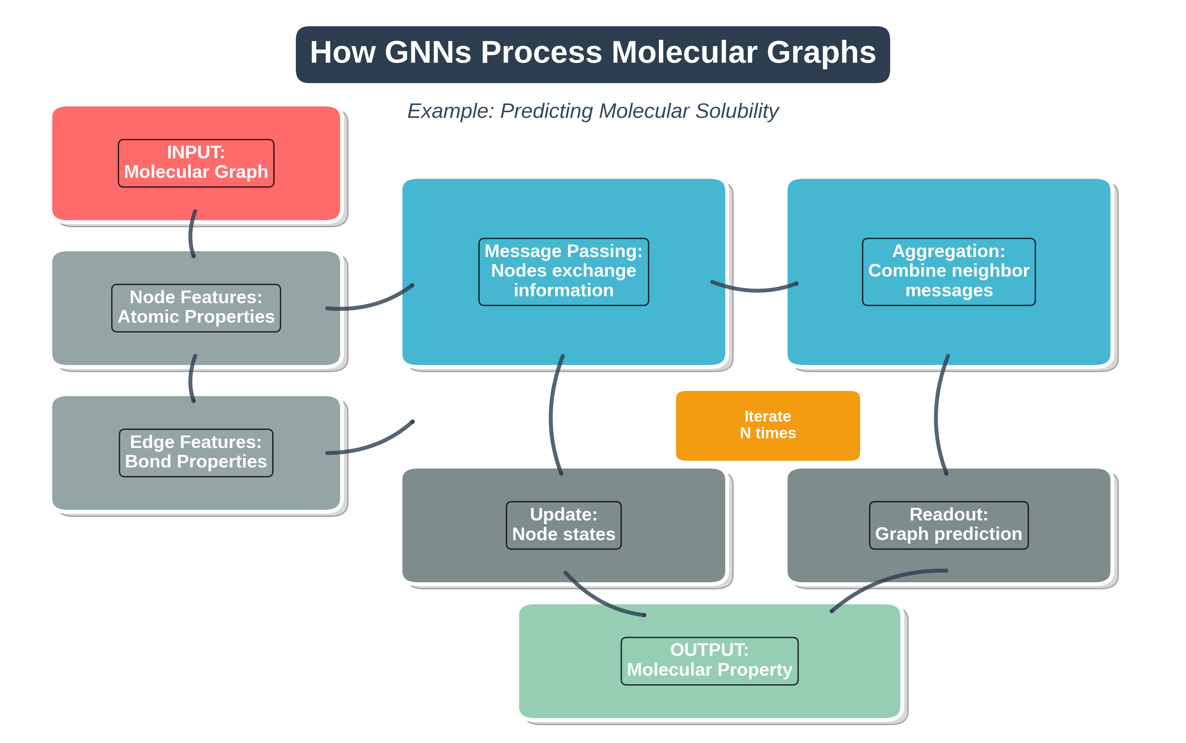
Graph neural networks (GNNs) are artificial neural networks designed for tasks whose inputs are graphs. Because graphs usually do not have a canonical ordering of their nodes, GNN architectures are commonly designed to be permutation equivariant: reordering the nodes in the input reorders the corresponding node representations in the same way. For graph-level prediction tasks, GNNs typically use a permutation-invariant readout function, whose output is unchanged by the ordering of the nodes. A prominent example is molecular drug design. Molecules can be represented as graphs, with nodes for atoms and edges for atomic bonds, often including known chemical properties as features. Inputs may thus differ in size, due to varying number of atoms and bonds. A graph-level task may be to predict the efficacy of a given molecule for a specific medical application, such as eliminating E. coli bacteria. The key design element of GNNs is the use of pairwise message passing, such that graph nodes iteratively update their representations by exchanging information with their neighbors. Several GNN architectures have been proposed, which implement different flavors of message passing, started by recursive or convolutional constructive approaches. A 2022 position paper argued that many architectures described as going "beyond" message passing can instead be interpreted as message passing over suitably modified graphs, and proposed the term "augmented message passing" for such approaches.
In the more general subject of "geometric deep learning", certain existing neural network architectures can be interpreted as GNNs operating on suitably defined graphs. A convolutional neural network layer, in the context of computer vision, can be considered a GNN applied to graphs whose nodes are pixels, and only adjacent pixels are connected by edges in the graph. A transformer layer, in natural language processing, can be considered a GNN applied to complete graphs whose nodes are words or tokens in a passage of natural language text. Relevant application domains for GNNs include natural language processing, social networks, citation networks, molecular biology, chemistry, physics and NP-hard combinatorial optimization problems. Open source libraries implementing GNNs include PyTorch Geometric (PyTorch), TensorFlow GNN (TensorFlow), Deep Graph Library (framework agnostic), jraph (Google JAX), and GraphNeuralNetworks.jl/GeometricFlux.jl (Julia, Flux).
Permutation-equivariant layers: a permutation equivariant layer maps a representation of a graph into an updated representation of the same graph. In the literature, permutation equivariant layers are implemented via pairwise message passing between graph nodes. Intuitively, in a message passing layer, nodes update their representations by aggregating the messages received from their immediate neighbours. As such, each message passing layer increases the receptive field of the GNN by one hop. Local pooling: a local pooling layer coarsens the graph via downsampling. Local pooling is used to increase the receptive field of a GNN, in a similar fashion to pooling layers in convolutional neural networks. Examples include k-nearest neighbours pooling, top-k pooling, and self-attention pooling. Global pooling: a global pooling layer, also known as readout layer, provides fixed-size representation of the whole graph. The global pooling layer must be permutation invariant, such that permutations in the ordering of graph nodes and edges do not alter the final output. Examples include element-wise sum, mean or maximum. Standard message-passing GNNs are at most as expressive as the Weisfeiler Leman graph isomorphism test. In practice, this means that there exist different graph structures that cannot be distinguished by GNNs. More powerful GNNs operating on higher-dimension geometries such as simplicial complexes can be designed. As of 2022, whether or not future architectures will overcome the message passing primitive is an open research question.
Message passing layers are permutation-equivariant layers mapping a graph into an updated representation of the same graph. Formally, they can be expressed as message passing neural networks (MPNNs). Let G = ( V , E ) {\displaystyle G=(V,E)} be a graph, where V {\displaystyle V} is the node set and E {\displaystyle E} is the edge set. Let N u {\displaystyle N_{u}} be the neighbourhood of some node u ∈ V {\displaystyle u\in V} . Additionally, let x u {\displaystyle \mathbf {x} _{u}} be the features of node u ∈ V {\displaystyle u\in V} , and e u v {\displaystyle \mathbf {e} _{uv}} be the features of edge ( u , v ) ∈ E {\displaystyle (u,v)\in E} . An MPNN layer can be expressed as follows:
h u = ϕ ( x u , ⨁ v ∈ N u ψ ( x u , x v , e u v ) ) {\displaystyle \mathbf {h} _{u}=\phi \left(\mathbf {x} _{u},\bigoplus _{v\in N_{u}}\psi (\mathbf {x} _{u},\mathbf {x} _{v},\mathbf {e} _{uv})\right)}
where ϕ {\displaystyle \phi } and ψ {\displaystyle \psi } are differentiable functions (e.g., artificial neural networks), and ⨁ {\displaystyle \bigoplus } is a permutation invariant aggregation operator that can accept an arbitrary number of inputs (e.g., element-wise sum, mean, or max). In particular, ϕ {\displaystyle \phi } and ψ {\displaystyle \psi } are referred to as update and message functions, respectively. Intuitively, in an MPNN computational block, graph nodes update their representations by aggregating the messages received from their neighbours. The outputs of one or more MPNN layers are node representations h u {\displaystyle \mathbf {h} _{u}} for each node u ∈ V {\displaystyle u\in V} in the graph. Node representations can be employed for any downstream task, such as node/graph classification or edge prediction. Graph nodes in an MPNN update their representation aggregating information from their immediate neighbours. As such, stacking n {\displaystyle n} MPNN layers means that one node will be able to communicate with nodes that are at most n {\displaystyle n} "hops" away. In principle, to ensure that every node receives information from every other node, one would need to stack a number of MPNN layers equal to the graph diameter. However, stacking many MPNN layers may cause issues such as oversmoothing and oversquashing. Oversmoothing refers to the issue of node representations becoming indistinguishable. Oversquashing refers to the bottleneck that is created by squeezing long-range dependencies into fixed-size representations. Countermeasures such as skip connections (as in residual neural networks), gated update rules and jumping knowledge can mitigate oversmoothing. Modifying the final layer to be a fully-adjacent layer, i.e., by considering the graph as a complete graph, can mitigate oversquashing in problems where long-range dependencies are required. Other "flavours" of MPNN have been developed in the literature, such as graph convolutional networks and graph attention networks, whose definitions can be expressed in terms of the MPNN formalism.
H = σ ( D ~ − 1 2 A ~ D ~ − 1 2 X Θ ) {\displaystyle \mathbf {H} =\sigma \left({\tilde {\mathbf {D} }}^{-{\frac {1}{2}}}{\tilde {\mathbf {A} }}{\tilde {\mathbf {D} }}^{-{\frac {1}{2}}}\mathbf {X} \mathbf {\Theta } \right)}
2. Related Work, Literature Survey & Algorithmic Foundations
where H {\displaystyle \mathbf {H} } is the matrix of node representations h u {\displaystyle \mathbf {h} _{u}} , X {\displaystyle \mathbf {X} } is the matrix of node features x u {\displaystyle \mathbf {x} _{u}} , σ ( ⋅ ) {\displaystyle \sigma (\cdot )} is an activation function (e.g., ReLU), A ~ {\displaystyle {\tilde {\mathbf {A} }}} is the graph adjacency matrix with the addition of self-loops, D ~ {\displaystyle {\tilde {\mathbf {D} }}} is the graph degree matrix with the addition of self-loops, and Θ {\displaystyle \mathbf {\Theta } } is a matrix of trainable parameters. In particular, let A {\displaystyle \mathbf {A} } be the graph adjacency matrix: then, one can define A ~ = A + I {\displaystyle {\tilde {\mathbf {A} }}=\mathbf {A} +\mathbf {I} } and D ~ i i = ∑ j ∈ V A ~ i j {\displaystyle {\tilde {\mathbf {D} }}_{ii}=\sum _{j\in V}{\tilde {A}}_{ij}} , where I {\displaystyle \mathbf {I} } denotes the identity matrix. This normalization ensures that the eigenvalues of D ~ − 1 2 A ~ D ~ − 1 2 {\displaystyle {\tilde {\mathbf {D} }}^{-{\frac {1}{2}}}{\tilde {\mathbf {A} }}{\tilde {\mathbf {D} }}^{-{\frac {1}{2}}}} are bounded in the range [ 0 , 1 ] {\displaystyle [0,1]} , avoiding numerical instabilities and exploding/vanishing gradients. A limitation of GCNs is that they do not allow multidimensional edge features e u v {\displaystyle \mathbf {e} _{uv}} . It is however possible to associate scalar weights w u v {\displaystyle w_{uv}} to each edge by imposing A u v = w u v {\displaystyle A_{uv}=w_{uv}} , i.e., by setting each nonzero entry in the adjacency matrix equal to the weight of the corresponding edge.
h u = ‖ k = 1 K σ ( ∑ v ∈ N u α u v k W k x v ) {\displaystyle \mathbf {h} _{u}={\overset {K}{\underset {k=1}{\Big \Vert }}}\sigma \left(\sum _{v\in N_{u}}\alpha _{uv}^{k}\mathbf {W} ^{k}\mathbf {x} _{v}\right)}
where K {\displaystyle K} is the number of attention heads, ‖ {\displaystyle {\Big \Vert }} denotes vector concatenation, σ ( ⋅ ) {\displaystyle \sigma (\cdot )} is an activation function (e.g., ReLU), N u {\displaystyle N_{u}} is the set of immediate neighbor nodes of node u {\displaystyle u} , including node u {\displaystyle u} itself, α u v k {\displaystyle \alpha _{uv}^{k}} are attention coefficients for the k {\displaystyle k} -th attention head, and W k {\displaystyle W^{k}} is a matrix of trainable parameters for the k {\displaystyle k} -th attention head. For the final GAT layer, the outputs from each attention head are averaged before the application of the activation function. Formally, the final GAT layer can be written as:
h u = σ ( 1 K ∑ k = 1 K ∑ v ∈ N u α u v k W k x v ) {\displaystyle \mathbf {h} _{u}=\sigma \left({\frac {1}{K}}\sum _{k=1}^{K}\sum _{v\in N_{u}}\alpha _{uv}^{k}\mathbf {W} ^{k}\mathbf {x} _{v}\right)}
Attention in Machine Learning is a technique that mimics cognitive attention. In the context of learning on graphs, the attention coefficient α u v {\displaystyle \alpha _{uv}} measures how important node v {\displaystyle v} is to node u {\displaystyle u} . Normalized attention coefficients are computed as follows:
α u v = exp ( LeakyReLU ( a T [ W x u ‖ W x v ‖ e u v ] ) ) ∑ z ∈ N u exp ( LeakyReLU ( a T [ W x u ‖ W x z ‖ e u z ] ) ) {\displaystyle \alpha _{uv}={\frac {\exp({\text{LeakyReLU}}\left(\mathbf {a} ^{T}[\mathbf {W} \mathbf {x} _{u}\Vert \mathbf {W} \mathbf {x} _{v}\Vert \mathbf {e} _{uv}]\right))}{\sum _{z\in N_{u}}\exp({\text{LeakyReLU}}\left(\mathbf {a} ^{T}[\mathbf {W} \mathbf {x} _{u}\Vert \mathbf {W} \mathbf {x} _{z}\Vert \mathbf {e} _{uz}]\right))}}}
where a {\displaystyle \mathbf {a} } is a vector of learnable weights, ⋅ T {\displaystyle \cdot ^{T}} indicates transposition, e u v {\displaystyle \mathbf {e} _{uv}} are the edge features (if present), and LeakyReLU {\displaystyle {\text{LeakyReLU}}} is a modified ReLU activation function. Attention coefficients are then normalized via softmax to make them easily comparable across different nodes. A GCN can be seen as a special case of a GAT where attention coefficients are not learnable, but fixed and equal to the edge weights w u v {\displaystyle w_{uv}} .
3. Dataset Ingestion, Preprocessing & Stochastic Augmentations
h u ( 0 ) = x u ‖ 0 {\displaystyle \mathbf {h} _{u}^{(0)}=\mathbf {x} _{u}\,\Vert \,\mathbf {0} }
m u ( l + 1 ) = ∑ v ∈ N u Θ h v {\displaystyle \mathbf {m} _{u}^{(l+1)}=\sum _{v\in N_{u}}\mathbf {\Theta } \mathbf {h} _{v}}
h u ( l + 1 ) = GRU ( m u ( l + 1 ) , h u ( l ) ) {\displaystyle \mathbf {h} _{u}^{(l+1)}={\text{GRU}}(\mathbf {m} _{u}^{(l+1)},\mathbf {h} _{u}^{(l)})}
where ‖ {\displaystyle \Vert } denotes vector concatenation, 0 {\displaystyle \mathbf {0} } is a vector of zeros, Θ {\displaystyle \mathbf {\Theta } } is a matrix of learnable parameters, GRU {\displaystyle {\text{GRU}}} is a GRU cell, and l {\displaystyle l} denotes the sequence index. In a GGS-NN, the node representations are regarded as the hidden states of a GRU cell. The initial node features x u ( 0 ) {\displaystyle \mathbf {x} _{u}^{(0)}} are zero-padded up to the hidden state dimension of the GRU cell. The same GRU cell is used for updating representations for each node.
Z = GNN e m b e d ( X , A ) {\displaystyle \mathbf {Z} =\operatorname {GNN} _{\mathrm {embed} }(\mathbf {X} ,\mathbf {A} )}
S = softmax ( GNN p o o l ( X , A ) ) {\displaystyle \mathbf {S} =\operatorname {softmax} (\operatorname {GNN} _{\mathrm {pool} }(\mathbf {X} ,\mathbf {A} ))}
where S i j {\displaystyle S_{ij}} denotes the soft assignment of node i {\displaystyle i} to cluster j {\displaystyle j} . The coarsened node-feature matrix and adjacency matrix are then computed as
4. Neural Network Backbone, Layer Specifications & Loss Formulations
X ′ = S T Z {\displaystyle \mathbf {X} '=\mathbf {S} ^{T}\mathbf {Z} }
A ′ = S T A S {\displaystyle \mathbf {A} '=\mathbf {S} ^{T}\mathbf {A} \mathbf {S} }
In this formulation, each new node in X ′ {\displaystyle \mathbf {X} '} represents a learned cluster of nodes from the previous graph, and edges in A ′ {\displaystyle \mathbf {A} '} represent aggregate connectivity between clusters. Because the assignment matrix is differentiable, DiffPool can be trained end-to-end together with the surrounding GNN layers. The original formulation additionally introduced auxiliary losses to encourage nearby nodes to be assigned to similar clusters and to encourage confident cluster assignments.
X ′ = ( X ⊙ sigmoid ( y ) ) i {\displaystyle \mathbf {X} '=(\mathbf {X} \odot {\text{sigmoid}}(\mathbf {y} ))_{\mathbf {i} }}
A ′ = A i , i {\displaystyle \mathbf {A} '=\mathbf {A} _{\mathbf {i} ,\mathbf {i} }}
where i = top k ( y ) {\displaystyle \mathbf {i} ={\text{top}}_{k}(\mathbf {y} )} is the subset of nodes with the top-k highest projection scores, ⊙ {\displaystyle \odot } denotes element-wise matrix multiplication, and sigmoid ( ⋅ ) {\displaystyle {\text{sigmoid}}(\cdot )} is the sigmoid function. In other words, the nodes with the top-k highest projection scores are retained in the new adjacency matrix A ′ {\displaystyle \mathbf {A} '} . The sigmoid ( ⋅ ) {\displaystyle {\text{sigmoid}}(\cdot )} operation makes the projection vector p {\displaystyle \mathbf {p} } trainable by backpropagation, which otherwise would produce discrete outputs.
X ′ = ( X ⊙ y ) i {\displaystyle \mathbf {X} '=(\mathbf {X} \odot \mathbf {y} )_{\mathbf {i} }}
5. Training Protocol, Convergence Behavior & Experimental Evaluation
A ′ = A i , i {\displaystyle \mathbf {A} '=\mathbf {A} _{\mathbf {i} ,\mathbf {i} }}
where i = top k ( y ) {\displaystyle \mathbf {i} ={\text{top}}_{k}(\mathbf {y} )} is the subset of nodes with the top-k highest projection scores, ⊙ {\displaystyle \odot } denotes element-wise matrix multiplication. The self-attention pooling layer can be seen as an extension of the top-k pooling layer. Differently from top-k pooling, the self-attention scores computed in self-attention pooling account both for the graph features and the graph topology.
Social networks are a major application domain for GNNs due to their natural representation as social graphs. GNNs are used to develop recommender systems based on both social relations and item relations.
GNNs are used as fundamental building blocks for several combinatorial optimization algorithms. Examples include computing shortest paths or Eulerian circuits for a given graph, deriving chip placements superior or competitive to handcrafted human solutions, and improving expert-designed branching rules in branch and bound.
When viewed as a graph, a network of computers can be analyzed with GNNs for anomaly detection. Anomalies within provenance graphs often correlate to malicious activity within the network. GNNs have been used to identify these anomalies on individual nodes and within paths to detect malicious processes, or on the edge level to detect lateral movement.
Water distribution systems can be modeled as graphs. GNNs have been applied to water demand forecasting, interconnecting District Metered Areas (DMAs) to improve the forecasting capacity. Another application is the development of metamodels.
To represent an image as a graph structure, the image is first divided into multiple patches, each of which is treated as a node in the graph. Edges are then formed by connecting each node to its nearest neighbors based on spatial or feature similarity. This graph-based representation enables the application of graph learning models to visual tasks. The relational structure helps to enhance feature extraction and improve performance on image understanding.
Model Figures & Evaluation Curves (4 Images)
Deep Learning Execution Pipeline
(Preprocessing)
(Feature Extraction)
(Self-Attention)
(Loss Optimization)