Complete Technical Paper Content — Gru Sequence Models
1. Executive Abstract, Problem Formulation & Background
In machine learning, attention is a method that determines the importance of, or "attends to", each component in a sequence relative to the other components in that sequence. In natural language processing, importance is represented by "soft" weights assigned to each word in a sentence. More generally, attention encodes vectors called token embeddings across a fixed-width sequence that can range from tens to millions of tokens in size. Unlike "hard" weights, which are computed during the backwards training pass, "soft" weights exist only in the forward pass and therefore change with every step of the input. Earlier designs implemented the attention mechanism in a serial recurrent neural network (RNN) language translation system, but a more recent design, namely the transformer, removed the slower sequential RNN and relied more heavily on the faster parallel attention scheme. Inspired by ideas about attention in humans, the attention mechanism was developed to address the weaknesses of using information from the hidden layers of recurrent neural networks. Recurrent neural networks favor information contained in words at the end of a sentence and thus deemed more recent, thereby tending to attenuate the significance and associated predictive weight assigned to information earlier in the sentence. Attention allows a token equal access to any part of a sentence directly, rather than only through the previous state.
Additional surveys of the attention mechanism in deep learning are provided by Niu et al. and Soydaner. The major breakthrough came with self-attention, where each element in the input sequence attends to all others, enabling the model to capture global dependencies. This idea was central to the Transformer architecture, which replaced recurrence with attention mechanisms. As a result, Transformers became the foundation for models like BERT, T5 and generative pre-trained transformers (GPT).
The modern era of machine attention was revitalized by grafting an attention mechanism (Fig 1. orange) to an Encoder-Decoder.
Sometimes, alignment can be multiple-to-multiple. For example, the English phrase look it up corresponds to cherchez-le. Thus, "soft" attention weights work better than "hard" attention weights (setting one attention weight to 1, and the others to 0), as we would like the model to make a context vector consisting of a weighted sum of the hidden vectors, rather than "the best one", as there may not be a best hidden vector.
fast weight programmers, or fast weight controllers (1992). A "slow" neural network outputs the "fast" weights of another neural network through outer products. The slow network learns by gradient descent. It was later renamed as "linearized self-attention". Bahdanau-style attention, also referred to as additive attention, Luong-style attention, which is known as multiplicative attention, Early attention mechanisms similar to modern self-attention were proposed using recurrent neural networks. However, the highly parallelizable self-attention was introduced in 2017 and successfully used in the Transformer model, positional attention and factorized positional attention. For convolutional neural networks, attention mechanisms can be distinguished by the dimension on which they operate, namely: spatial attention, channel attention, or combinations. These variants recombine the encoder-side inputs to redistribute those effects to each target output. Often, a correlation-style matrix of dot products provides the re-weighting coefficients. In the figures below, W is the matrix of context attention weights, similar to the formula in Overview section above.
From the original paper on vision transformers (ViT), visualizing attention scores as a heat map (called saliency maps or attention maps) has become an important and routine way to inspect the decision making process of ViT models. One can compute the attention maps with respect to any attention head at any layer, while the deeper layers tend to show more semantically meaningful visualization. Attention rollout is a recursive algorithm to combine attention scores across all layers, by computing the dot product of successive attention maps. Because vision transformers are typically trained in a self-supervised manner, attention maps are generally not class-sensitive. When a classification head is attached to the ViT backbone, class-discriminative attention maps (CDAM) combines attention maps and gradients with respect to the class [CLS] token. Some class-sensitive interpretability methods originally developed for convolutional neural networks can be also applied to ViT, such as GradCAM, which back-propagates the gradients to the outputs of the final attention layer. Using attention as basis of explanation for the transformers in language and vision is not without debate. While some pioneering papers analyzed and framed attention scores as explanations, higher attention scores do not always correlate with greater impact on model performances.
Attention ( Q , K , V ) = softmax ( Q K T d k ) V ∈ R m × d v {\displaystyle {\text{Attention}}(Q,K,V)={\text{softmax}}\left({\frac {QK^{T}}{\sqrt {d_{k}}}}\right)V\in \mathbb {R} ^{m\times d_{v}}}
T {\displaystyle {}^{T}} denotes transpose and the softmax function is applied independently to every row of its argument. The matrix Q {\displaystyle Q} contains m {\displaystyle m} queries, while matrices K , V {\displaystyle K,V} jointly contain an unordered set of n {\displaystyle n} key-value pairs. Value vectors in matrix V {\displaystyle V} are weighted using the weights resulting from the softmax operation, so that the rows of the m {\displaystyle m} -by- d v {\displaystyle d_{v}} output matrix are confined to the convex hull of the points in R d v {\displaystyle \mathbb {R} ^{d_{v}}} given by the rows of V {\displaystyle V} . To understand the permutation invariance and permutation equivariance properties of QKV attention, let A ∈ R m × m {\displaystyle A\in \mathbb {R} ^{m\times m}} and B ∈ R n × n {\displaystyle B\in \mathbb {R} ^{n\times n}} be permutation matrices; and D ∈ R m × n {\displaystyle D\in \mathbb {R} ^{m\times n}} an arbitrary matrix. The softmax function is permutation equivariant in the sense that:
softmax ( A D B ) = A softmax ( D ) B {\displaystyle {\text{softmax}}(ADB)=A\,{\text{softmax}}(D)B}
2. Related Work, Literature Survey & Algorithmic Foundations
Attention ( A Q , B K , B V ) = A Attention ( Q , K , V ) {\displaystyle {\text{Attention}}(AQ,BK,BV)=A\,{\text{Attention}}(Q,K,V)}
which shows that QKV attention is equivariant with respect to re-ordering the queries (rows of Q {\displaystyle Q} ); and invariant to re-ordering of the key-value pairs in K , V {\displaystyle K,V} . These properties are inherited when applying linear transforms to the inputs and outputs of QKV attention blocks. For example, a simple self-attention function defined as:
X ↦ Attention ( X T q , X T k , X T v ) {\displaystyle X\mapsto {\text{Attention}}(XT_{q},XT_{k},XT_{v})} is permutation equivariant with respect to re-ordering the rows of the input matrix X {\displaystyle X} in a non-trivial way, because every row of the output is a function of all the rows of the input. Similar properties hold for multi-head attention, which is defined below.
Attention ( Q , K , V ) = softmax ( Q K T d k + M ) V {\displaystyle {\text{Attention}}(Q,K,V)={\text{softmax}}\left({\frac {QK^{T}}{\sqrt {d_{k}}}}+M\right)V}
where the mask, M ∈ { 0 , − ∞ } n × n {\displaystyle M\in \mathbb {\{0,-\infty \}} ^{n\times n}} is a strictly upper triangular matrix, with zeros on and below the diagonal and − ∞ {\displaystyle -\infty } in every element above the diagonal. The softmax output, in R n × n {\displaystyle \mathbb {R} ^{n\times n}} is then lower triangular, with zeros in all elements above the diagonal. The masking ensures that for all 1 ≤ i < j ≤ n {\displaystyle 1\leq i<j\leq n} , row i {\displaystyle i} of the attention output is independent of row j {\displaystyle j} of any of the three input matrices. The permutation invariance and equivariance properties of standard QKV attention do not hold for the masked variant.
MultiHead ( Q , K , V ) = Concat ( head 1 , . . . , head h ) W O {\displaystyle {\text{MultiHead}}(Q,K,V)={\text{Concat}}({\text{head}}_{1},...,{\text{head}}_{h})W^{O}}
head i = Attention ( Q W i Q , K W i K , V W i V ) {\displaystyle {\text{head}}_{i}={\text{Attention}}(QW_{i}^{Q},KW_{i}^{K},VW_{i}^{V})}
and W i Q , W i K , W i V {\displaystyle W_{i}^{Q},W_{i}^{K},W_{i}^{V}} , and W O {\displaystyle W^{O}} are parameter matrices. The permutation properties of (standard, unmasked) QKV attention apply here also. For permutation matrices, A , B {\displaystyle A,B} :
MultiHead ( A Q , B K , B V ) = A MultiHead ( Q , K , V ) {\displaystyle {\text{MultiHead}}(AQ,BK,BV)=A\,{\text{MultiHead}}(Q,K,V)}
3. Dataset Ingestion, Preprocessing & Stochastic Augmentations
X ↦ MultiHead ( X T q , X T k , X T v ) {\displaystyle X\mapsto {\text{MultiHead}}(XT_{q},XT_{k},XT_{v})} is equivariant with respect to re-ordering of the rows of input matrix X {\displaystyle X} .
Attention ( Q , K , V ) = softmax ( tanh ( W Q Q + W K K ) ) V {\displaystyle {\text{Attention}}(Q,K,V)={\text{softmax}}(\tanh(W_{Q}Q+W_{K}K))V}
where W Q {\displaystyle W_{Q}} and W K {\displaystyle W_{K}} are learnable weight matrices.
Attention ( Q , K , V ) = softmax ( Q W K T ) V {\displaystyle {\text{Attention}}(Q,K,V)={\text{softmax}}(QWK^{T})V}
where W {\displaystyle W} is a learnable weight matrix.
A generative pre-trained transformer (GPT) is a type of large language model (LLM) that is widely used in generative artificial intelligence chatbots. GPTs are based on a deep learning architecture called the transformer. They are pre-trained on large datasets of unlabeled content, and able to generate novel content. OpenAI was the first to apply generative pre-training to the transformer architecture, introducing the GPT-1 model in 2018. The chatbot ChatGPT, released in late 2022 (using GPT-3.5), was followed by many competitor chatbots using their own generative pre-trained transformers to generate text, such as Gemini, DeepSeek and Claude. GPTs are primarily used to generate text, but can be trained to generate other kinds of data. Multimodal GPTs can process or generate multiple types of data, such as text, images and audio. To improve performance on complex tasks, reasoning GPTs allocate more computation time analyzing the problem before generating an output.
OpenAI, which created the first generative pre-trained transformer (GPT) in 2018, asserted in 2023 that "GPT" should be regarded as a brand of OpenAI. In April 2023, OpenAI revised the brand guidelines in its terms of service to indicate that other businesses using its API to run their AI services would no longer be able to include "GPT" in such names or branding. In May 2023, OpenAI engaged a brand management service to notify its API customers of this policy, although these notifications stopped short of making overt legal claims (such as allegations of trademark infringement or demands to cease and desist). As of November 2023, OpenAI still prohibits its API licensees from naming their own products with "GPT", but it has begun enabling its ChatGPT Plus subscribers to make "custom versions of ChatGPT" called GPTs on the OpenAI site. OpenAI's terms of service says that its subscribers may use "GPT" in the names of these, although it is "discouraged". Relatedly, OpenAI has applied to the United States Patent and Trademark Office (USPTO) to seek domestic trademark registration for the term "GPT" in the field of AI. OpenAI sought to expedite handling of its application, but the USPTO declined that request in April 2023. In May 2023, the USPTO rejected OpenAI's trademark application, determining that "GPT" was both descriptive and generic. In the European Union, the European Union Intellectual Property Office registered "GPT" as a trade mark of OpenAI in spring 2023. However, since spring 2024 the registration is being challenged and is pending cancellation. In Switzerland, the Swiss Federal Institute of Intellectual Property registered "GPT" as a trade mark of OpenAI in spring 2023. The China National Intellectual Property Administration denied OpenAI's applications to trademark the terms "GPT" and "ChatGPT" in 2024, and the term "GPT-5" in August 2025, after which OpenAI filed appeals.
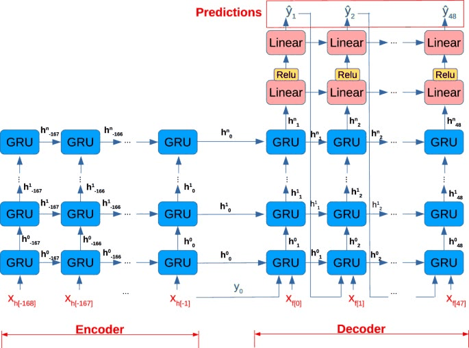
GRU Model from Scratch This repository demonstrates how to implement a Gated Recurrent Unit (GRU) model from scratch using PyTorch. The notebook provides a step-by-step guide to building and training a GRU-based sequence-to-sequence (Seq2Seq) model. You'll learn how to preprocess data, design custom GRU gates, and train the model effectively. Notebook Sections Import Relevant Libraries Load libraries required for data preprocessing, model building, and training. Tokenize Words & Preprocess Dataset Tokenize and preprocess text data for the GRU model. Build Vocabulary & Numericalize Data Create a vocabulary and convert tokenized data into numerical form. Design GRU Module Build GRU gates (reset, update, and candidate hidden state) and complete the GRU cell. Build Seq2Seq Model Combine the encoder and decoder modules for sequence-to-sequence modeling. Train the Model Train the model using a custom training loop and visualize training progress. Training and Validation Below is the training and validation loss graph for the GRU model: Results Here are some sample predictions made by the model: Predicted Correct A man with a hat hat is working on his face. A man in an orange hat staring at something. A is walking through a green grass with a red ball. A Boston terrier is running on lush green grass in front of a white fence. A girl in a is a a a a. A girl in karate uniform breaking a stick with a front kick. People in in in a room with a and and in in the background. Five people wearing winter jackets and helmets stand in the snow, with in the background. People are walking on a street. People are fixing the roof of a house. A man in a in a group of men, a man in a woman in a woman in a group of men and a woman in a background. A man in light-colored clothing photographs a group of men wearing dark suits and hats standing around a woman dressed in a gown. A group of people standing in front of a building. A group of people standing in front of an igloo. A boy in a red jersey is trying to kick the ball ball in the air while the other team in the background. A boy in a red uniform is attempting to avoid getting out at home plate, while the catcher in the blue uniform is attempting to catch him. A man is working on a . . A guy works on a building. A man in a red coat is sitting on a bench. A man in a vest is sitting in a chair and holding magazines. References This implementation is inspired by the following resources: PyTorch Seq2Seq Tutorials by Ben Trevett Original GRU Paper: "Learning Phrase Representations using RNN Encoder-Decoder for Statistical Machine Translation" License This project is licensed under the MIT License. See the LICENSE file for more details.
This repository demonstrates how to implement a Gated Recurrent Unit (GRU) model from scratch using PyTorch. The notebook provides a step-by-step guide to building and training a GRU-based sequence-to-sequence (Seq2Seq) model. You'll learn how to preprocess data, design custom GRU gates, and train the model effectively.
4. Neural Network Backbone, Layer Specifications & Loss Formulations
Import Relevant Libraries Load libraries required for data preprocessing, model building, and training.
Tokenize Words & Preprocess Dataset Tokenize and preprocess text data for the GRU model.
Build Vocabulary & Numericalize Data Create a vocabulary and convert tokenized data into numerical form.
Design GRU Module Build GRU gates (reset, update, and candidate hidden state) and complete the GRU cell.
Build Seq2Seq Model Combine the encoder and decoder modules for sequence-to-sequence modeling.
Train the Model Train the model using a custom training loop and visualize training progress.
This project is licensed under the MIT License. See the LICENSE file for more details.
This repository provides a step-by-step implementation of a Gated Recurrent Unit (GRU) model from scratch using PyTorch.
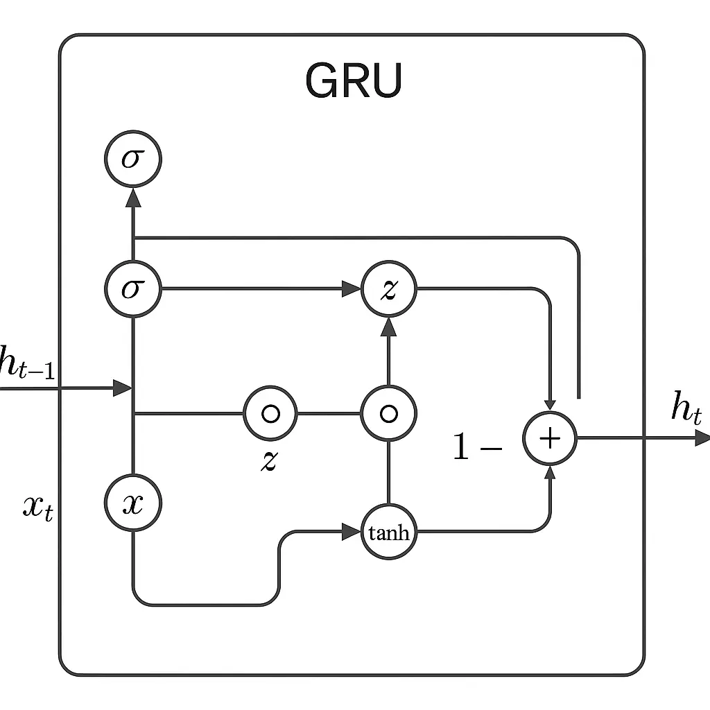
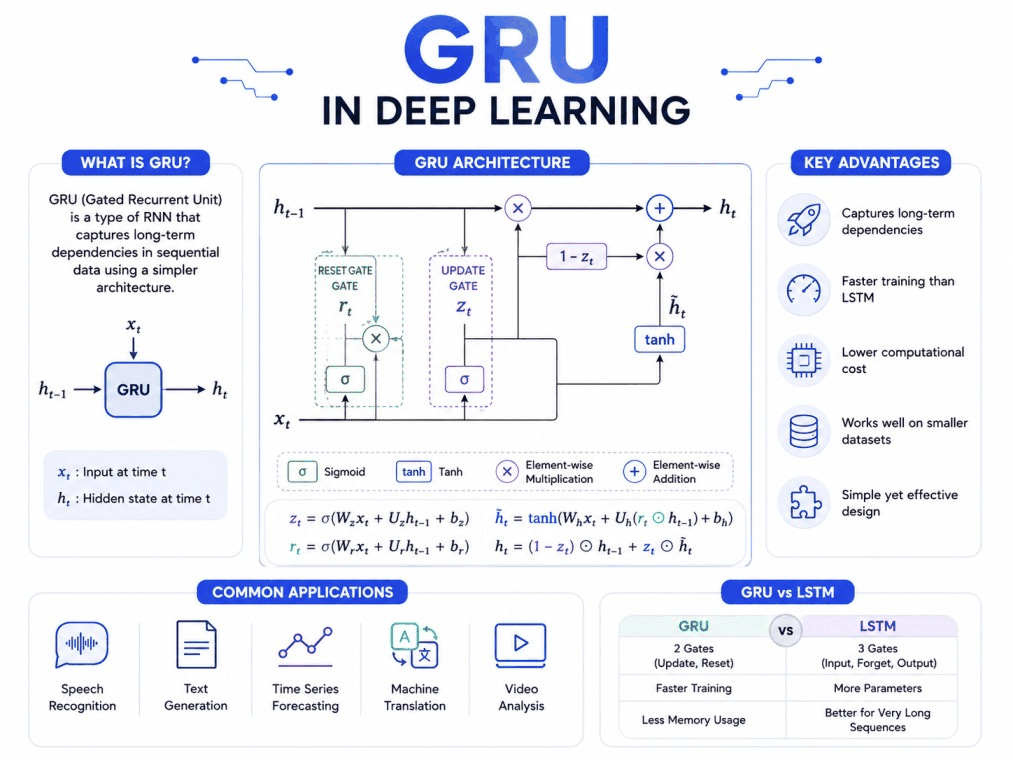
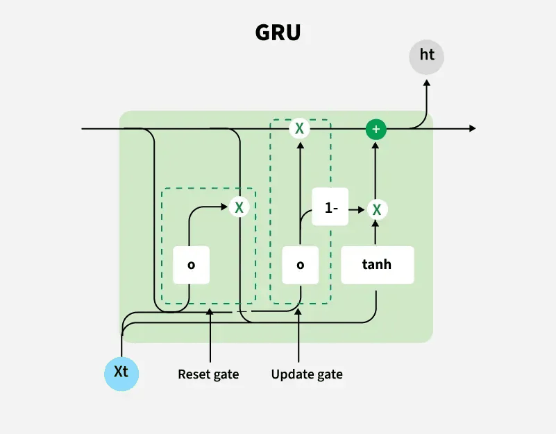
Table of Contents # Fundamental Concepts of GRU Implementing GRU from Scratch in PyTorch Usage Methods Common Practices Best Practices Conclusion References 1. Fundamental Concepts of GRU # What is a GRU? # A GRU is a type of RNN that has gating mechanisms to control the flow of information. It consists of two main gates: the reset gate ($r$) and the update gate ($z$). Reset Gate ($r$) : Determines how much of the previous hidden state should be forgotten. It is calculated as: [r_t = \sigma(W_r[x_t, h_{t - 1}] + b_r)] where $x_t$ is the input at time step $t$, $h_{t - 1}$ is the previous hidden state, $W_r$ is the weight matrix for the reset gate, $b_r$ is the bias, and $\sigma$ is the sigmoid function. Update Gate ($z$) : Decides whether to update the previous hidden state or keep it. It is calculated as: [z_t = \sigma(W_z[x_t, h_{t - 1}] + b_z)] Candidate Hidden State ($\tilde{h}_t$) : It is a candidate for the new hidden state and is calculated using the reset gate: [\tilde{h} t = \tanh(W_h[x_t, r_t \odot h {t - 1}] + b_h)] Final Hidden State ($h_t$) : The new hidden state is a combination of the previous hidden state and the candidate hidden state, controlled by the update gate: [h_t=(1 - z_t)\odot\tilde{h} t+z_t\odot h {t - 1}] 2. Implementing GRU from Scratch in PyTorch # import torch import torch.nn as nn class GRUFromScratch ( nn . Module ): def __init__ (self, input_size, hidden_size): super (GRUFromScratch, self ). __init__ () self .input_size = input_size self .hidden_size = hidden_size # Reset gate parameters self .W_r = nn.Linear(input_size + hidden_size, hidden_size) # Update gate parameters self .W_z = nn.Linear(input_size + hidden_size, hidden_size) # Candidate hidden state parameters self .W_h = nn.Linear(input_size + hidden_size, hidden_size) def forward (self, x, h_prev): batch_size, seq_len, _ = x.size() h = h_prev outputs = [] for t in range (seq_len): x_t = x[:, t, :] combined = torch.cat((x_t, h), dim = 1 ) # Compute reset gate r = torch.sigmoid( self .W_r(combined)) # Compute update gate z = torch.sigmoid( self .W_z(combined)) # Compute candidate hidden state combined_reset = torch.cat((x_t, r * h), dim = 1 ) h_tilde = torch.tanh( self .W_h(combined_reset)) # Compute new hidden state h = ( 1 - z) * h_tilde + z * h outputs.append(h.unsqueeze( 1 )) outputs = torch.cat(outputs, dim = 1 ) return outputs, h # Example usage input_size = 10 hidden_size = 20 batch_size = 32 seq_len = 5 x = torch.randn(batch_size, seq_len, input_size) h_prev = torch.zeros(batch_size, hidden_size) gru = GRUFromScratch(input_size, hidden_size) outputs, h = gru(x, h_prev) print ( "Output shape:" , outputs.shape) print ( "Final hidden state shape:" , h.shape) 3. Usage Methods # Training a GRU Model # To train a GRU model, you typically follow these steps: Define the model : As shown in the previous code example, define a GRU class. Define the loss function : For classification tasks, you can use cross-entropy loss. For regression tasks, mean squared error loss can be used. Define the optimizer : Common optimizers include Adam, SGD, etc. Training loop : Iterate over the training data, compute the loss, and update the model parameters. import torch.optim as optim # Define the model input_size = 10 hidden_size = 20 gru = GRUFromScratch(input_size, hidden_size) # Define the loss function and optimizer criterion = nn.MSELoss() optimizer = optim.Adam(gru.parameters(), lr = 0.001 ) # Generate some dummy target data target = torch.randn(batch_size, seq_len, hidden_size) # Training loop num_epochs = 100 for epoch in range (num_epochs): optimizer.zero_grad() outputs, _ = gru(x, h_prev) loss = criterion(outputs, target) loss.backward() optimizer.step() if (epoch + 1 ) % 10 == 0 : print ( f 'Epoch [ { epoch + 1} / { num_epochs } ], Loss: { loss.item() :.4f } ' ) 4. Common Practices # Data Preprocessing # Normalization : Normalize the input data to have zero mean and unit variance. This helps the model converge faster. Sequence Padding : If the input sequences have different lengths, pad them to the same length. Hyperparameter Tuning # Learning Rate : Adjust the learning rate to find the optimal value for training. A too-large learning rate may cause the model to diverge, while a too-small learning rate may lead to slow convergence. Hidden Size : The hidden size of the GRU can significantly affect the model's performance. Try different hidden sizes to find the best one. 5. Best Practices # Initialization # Weight Initialization : Initialize the weights of the GRU properly. For example, you can use Xavier or He initialization. def init_weights (m): if isinstance (m, nn.Linear): nn.init.xavier_uniform_(m.weight) nn.init.zeros_(m.bias) gru.apply(init_weights) Regularization # Dropout : Add dropout layers to prevent overfitting. You can add dropout between the input and the GRU layer or between the GRU layers in a multi-layer GRU model. class GRUWithDropout ( nn . Module ): def __init__ (self, input_size, hidden_size, dropout_prob): super (GRUWithDropout, self ). __init__ () self .gru = GRUFromScratch(input_size, hidden_size) self .dropout = nn.Dropout(dropout_prob) def forward (self, x, h_prev): outputs, h = self .gru(x, h_prev) outputs = self .dropout(outputs) return outputs, h dropout_prob = 0.2 gru_with_dropout = GRUWithDropout(input_size, hidden_size, dropout_prob) 6. Conclusion # In this blog, we have covered the fundamental concepts of GRUs, implemented a GRU from scratch using PyTorch, explored usage methods, common practices, and best practices. GRUs are powerful models for handling sequential data, and understanding how to implement them from scratch can give you a deeper understanding of their working principles. By following the best practices, you can train more robust and efficient GRU models. 7. References # Cho, Kyunghyun, et al. "Learning phrase representations using RNN encoder-decoder for statistical machine translation." arXiv preprint arXiv:1406.1078 (2014). PyTorch official documentation: https://pytorch.org/docs/stable/index.html 2025-11
5. Training Protocol, Convergence Behavior & Experimental Evaluation
A GRU is a type of RNN that has gating mechanisms to control the flow of information. It consists of two main gates: the reset gate ($r$) and the update gate ($z$).
Reset Gate ($r$) : Determines how much of the previous hidden state should be forgotten. It is calculated as: [r_t = \sigma(W_r[x_t, h_{t - 1}] + b_r)] where $x_t$ is the input at time step $t$, $h_{t - 1}$ is the previous hidden state, $W_r$ is the weight matrix for the reset gate, $b_r$ is the bias, and $\sigma$ is the sigmoid function.
Update Gate ($z$) : Decides whether to update the previous hidden state or keep it. It is calculated as: [z_t = \sigma(W_z[x_t, h_{t - 1}] + b_z)]
Candidate Hidden State ($\tilde{h}_t$) : It is a candidate for the new hidden state and is calculated using the reset gate: [\tilde{h} t = \tanh(W_h[x_t, r_t \odot h {t - 1}] + b_h)]
Final Hidden State ($h_t$) : The new hidden state is a combination of the previous hidden state and the candidate hidden state, controlled by the update gate: [h_t=(1 - z_t)\odot\tilde{h} t+z_t\odot h {t - 1}]
import torch import torch.nn as nn class GRUFromScratch ( nn . Module ): def __init__ (self, input_size, hidden_size): super (GRUFromScratch, self ). __init__ () self .input_size = input_size self .hidden_size = hidden_size # Reset gate parameters self .W_r = nn.Linear(input_size + hidden_size, hidden_size) # Update gate parameters self .W_z = nn.Linear(input_size + hidden_size, hidden_size) # Candidate hidden state parameters self .W_h = nn.Linear(input_size + hidden_size, hidden_size) def forward (self, x, h_prev): batch_size, seq_len, _ = x.size() h = h_prev outputs = [] for t in range (seq_len): x_t = x[:, t, :] combined = torch.cat((x_t, h), dim = 1 ) # Compute reset gate r = torch.sigmoid( self .W_r(combined)) # Compute update gate z = torch.sigmoid( self .W_z(combined)) # Compute candidate hidden state combined_reset = torch.cat((x_t, r * h), dim = 1 ) h_tilde = torch.tanh( self .W_h(combined_reset)) # Compute new hidden state h = ( 1 - z) * h_tilde + z * h outputs.append(h.unsqueeze( 1 )) outputs = torch.cat(outputs, dim = 1 ) return outputs, h # Example usage input_size = 10 hidden_size = 20 batch_size = 32 seq_len = 5 x = torch.randn(batch_size, seq_len, input_size) h_prev = torch.zeros(batch_size, hidden_size) gru = GRUFromScratch(input_size, hidden_size) outputs, h = gru(x, h_prev) print ( "Output shape:" , outputs.shape) print ( "Final hidden state shape:" , h.shape)
import torch.optim as optim # Define the model input_size = 10 hidden_size = 20 gru = GRUFromScratch(input_size, hidden_size) # Define the loss function and optimizer criterion = nn.MSELoss() optimizer = optim.Adam(gru.parameters(), lr = 0.001 ) # Generate some dummy target data target = torch.randn(batch_size, seq_len, hidden_size) # Training loop num_epochs = 100 for epoch in range (num_epochs): optimizer.zero_grad() outputs, _ = gru(x, h_prev) loss = criterion(outputs, target) loss.backward() optimizer.step() if (epoch + 1 ) % 10 == 0 : print ( f 'Epoch [ { epoch + 1} / { num_epochs } ], Loss: { loss.item() :.4f } ' )
def init_weights (m): if isinstance (m, nn.Linear): nn.init.xavier_uniform_(m.weight) nn.init.zeros_(m.bias) gru.apply(init_weights)
class GRUWithDropout ( nn . Module ): def __init__ (self, input_size, hidden_size, dropout_prob): super (GRUWithDropout, self ). __init__ () self .gru = GRUFromScratch(input_size, hidden_size) self .dropout = nn.Dropout(dropout_prob) def forward (self, x, h_prev): outputs, h = self .gru(x, h_prev) outputs = self .dropout(outputs) return outputs, h dropout_prob = 0.2 gru_with_dropout = GRUWithDropout(input_size, hidden_size, dropout_prob)
Model Figures & Evaluation Curves (4 Images)
Deep Learning Execution Pipeline
(Preprocessing)
(Feature Extraction)
(Self-Attention)
(Loss Optimization)