Complete Technical Paper Content — Histopathology Image Analysis
1. Executive Abstract, Problem Formulation & Background
In statistics and machine learning, ensemble methods use multiple learning algorithms to obtain better predictive performance than could be obtained from any of the constituent learning algorithms alone. Unlike a statistical ensemble in statistical mechanics, which is usually infinite, a machine learning ensemble consists of only a concrete finite set of alternative models, but typically allows for much more flexible structure to exist among those alternatives.
Theoretically, one can justify the diversity concept because the lower bound of the error rate of an ensemble system can be decomposed into accuracy, diversity, and the other term.
The Bayes optimal classifier is a classification technique. It is an ensemble of all the hypotheses in the hypothesis space. On average, no other ensemble can outperform it. The Naive Bayes classifier is a version of this that assumes that the data is conditionally independent on the class and makes the computation more feasible. Each hypothesis is given a vote proportional to the likelihood that the training dataset would be sampled from a system if that hypothesis were true. To facilitate training data of finite size, the vote of each hypothesis is also multiplied by the prior probability of that hypothesis. The Bayes optimal classifier can be expressed with the following equation:
y = a r g m a x c j ∈ C ∑ h i ∈ H P ( c j | h i ) P ( T | h i ) P ( h i ) {\displaystyle y={\underset {c_{j}\in C}{\mathrm {argmax} }}\sum _{h_{i}\in H}{P(c_{j}|h_{i})P(T|h_{i})P(h_{i})}}
where y {\displaystyle y} is the predicted class, C {\displaystyle C} is the set of all possible classes, H {\displaystyle H} is the hypothesis space, P {\displaystyle P} refers to a probability, and T {\displaystyle T} is the training data. As an ensemble, the Bayes optimal classifier represents a hypothesis that is not necessarily in H {\displaystyle H} . The hypothesis represented by the Bayes optimal classifier, however, is the optimal hypothesis in ensemble space (the space of all possible ensembles consisting only of hypotheses in H {\displaystyle H} ). This formula can be restated using Bayes' theorem, which says that the posterior is proportional to the likelihood times the prior:
P ( h i | T ) ∝ P ( T | h i ) P ( h i ) {\displaystyle P(h_{i}|T)\propto P(T|h_{i})P(h_{i})}
y = a r g m a x c j ∈ C ∑ h i ∈ H P ( c j | h i ) P ( h i | T ) {\displaystyle y={\underset {c_{j}\in C}{\mathrm {argmax} }}\sum _{h_{i}\in H}{P(c_{j}|h_{i})P(h_{i}|T)}}
Boosting involves training successive models by emphasizing training data mis-classified by previously learned models. Initially, all data (D1) has equal weight and is used to learn a base model M1. The examples mis-classified by M1 are assigned a weight greater than correctly classified examples. This boosted data (D2) is used to train a second base model M2, and so on. Inference is done by voting. In some cases, boosting has yielded better accuracy than bagging, but tends to over-fit more. The most common implementation of boosting is Adaboost, but some newer algorithms are reported to achieve better results.
For each model m in the bucket: Do c times: (where 'c' is some constant) Randomly divide the training dataset into two sets: A and B Train m with A Test m with B Select the model that obtains the highest average score
Cross-Validation Selection can be summed up as: "try them all with the training set, and pick the one that works best". Gating is a generalization of Cross-Validation Selection. It involves training another learning model to decide which of the models in the bucket is best-suited to solve the problem. Often, a perceptron is used for the gating model. It can be used to pick the "best" model, or it can be used to give a linear weight to the predictions from each model in the bucket. When a bucket of models is used with a large set of problems, it may be desirable to avoid training some of the models that take a long time to train. Landmark learning is a meta-learning approach that seeks to solve this problem. It involves training only the fast (but imprecise) algorithms in the bucket, and then using the performance of these algorithms to help determine which slow (but accurate) algorithm is most likely to do best.
e k = H ( p , q k ) − λ K ∑ j ≠ k H ( q j , q k ) {\displaystyle e^{k}=H(p,q^{k})-{\frac {\lambda }{K}}\sum _{j\neq k}H(q^{j},q^{k})}
where e k {\displaystyle e^{k}} is the cost function of the k t h {\displaystyle k^{th}} classifier, q k {\displaystyle q^{k}} is the probability of the k t h {\displaystyle k^{th}} classifier, p {\displaystyle p} is the true probability that we need to estimate and λ {\displaystyle \lambda } is a parameter between 0 and 1 that define the diversity that we would like to establish. When λ = 0 {\displaystyle \lambda =0} we want each classifier to do its best regardless of the ensemble and when λ = 1 {\displaystyle \lambda =1} we would like the classifier to be as diverse as possible.
Face recognition, which recently has become one of the most popular research areas of pattern recognition, copes with identification or verification of a person by their digital images. Hierarchical ensembles based on Gabor Fisher classifier and independent component analysis preprocessing techniques are some of the earliest ensembles employed in this field.
While speech recognition is mainly based on deep learning because most of the industry players in this field like Google, Microsoft and IBM reveal that the core technology of their speech recognition is based on this approach, speech-based emotion recognition can also have a satisfactory performance with ensemble learning. It is also being successfully used in facial emotion recognition.
Fraud detection deals with the identification of bank fraud, such as money laundering, credit card fraud and telecommunication fraud, which have vast domains of research and applications of machine learning. Because ensemble learning improves the robustness of the normal behavior modelling, it has been proposed as an efficient technique to detect such fraudulent cases and activities in banking and credit card systems.
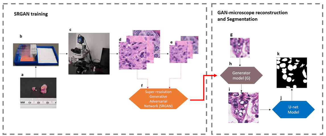
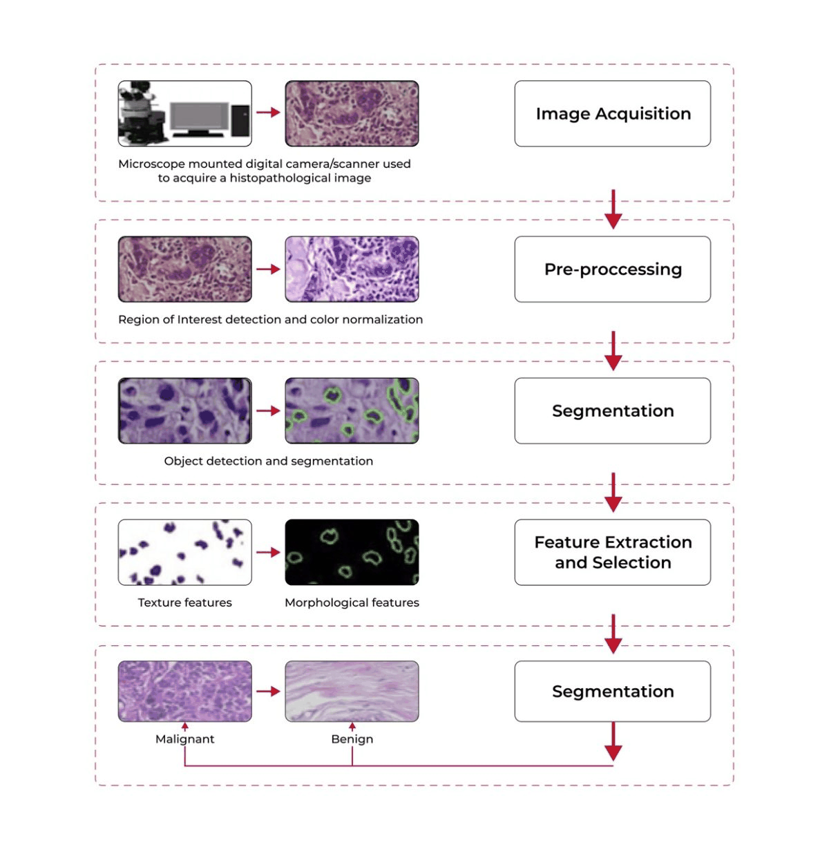
In digital image processing and computer vision, image segmentation is the process of partitioning a digital image into multiple image segments, also known as image regions or image objects (sets of pixels). The goal of segmentation is to simplify and/or change the representation of an image into something that is more meaningful and easier to analyze. Image segmentation is typically used to locate objects and boundaries (lines, curves, etc.) in images. More precisely, image segmentation is the process of assigning a label to every pixel in an image such that pixels with the same label share certain characteristics. The result of image segmentation is a set of segments that collectively cover the entire image, or a set of contours extracted from the image (see edge detection). Each of the pixels in a region are similar with respect to some characteristic or computed property, such as color, intensity, or texture. Adjacent regions are significantly different with respect to the same characteristic(s). When applied to a stack of images, typical in medical imaging, the resulting contours after image segmentation can be used to create 3D reconstructions with the help of geometry reconstruction algorithms like marching cubes.
2. Related Work, Literature Survey & Algorithmic Foundations
Content-based image retrieval Machine vision Medical imaging, and imaging studies in biomedical research, including volume rendered images from computed tomography, magnetic resonance imaging, as well as volume electron microscopy techniques such as FIB-SEM. Locate tumors and other pathologies Measure tissue volumes Diagnosis, study of anatomical structure Surgery planning Virtual surgery simulation Intra-surgery navigation Radiotherapy Digital Pathology and Histopathology. Nuclei instance segmentation in variously stained whole slide images (WSIs) refers to the automatic delineation of individual cells' nuclei borders. This task is a specialized subproblem of instance segmentation, with high practical importance in biomedical research and diagnostics (e.g. cell counting, morphometric feature extraction, tumor grading, prognostic biomarker extraction). The modern approach to the problem is the use of deep learning architectures developed to encompass the main challenges of separating overlapping or fused nuclei. The availability of few humanly-annotated datasets poses another challenge to the problem. Object detection Pedestrian detection Face detection Brake light detection Locate objects in satellite images (roads, forests, crops, etc.) Recognition Tasks Face recognition Fingerprint recognition Iris recognition Prohibited Item at Airport security checkpoints Traffic control systems Video surveillance Video object co-segmentation and action localization Several general-purpose algorithms and techniques have been developed for image segmentation. To be useful, these techniques must typically be combined with a domain's specific knowledge in order to effectively solve the domain's segmentation problems.
The simplest method of image segmentation is called the thresholding method. This method is based on a clip-level (or a threshold value) to turn a gray-scale image into a binary image. The key of this method is to select the threshold value (or values when multiple-levels are selected). Several popular methods are used in industry including the maximum entropy method, balanced histogram thresholding, Otsu's method (maximum variance), and k-means clustering. Recently, methods have been developed for thresholding computed tomography (CT) images. The key idea is that, unlike Otsu's method, the thresholds are derived from the radiographs instead of the (reconstructed) image. New methods suggest the use of multi-dimensional, fuzzy rule-based, non-linear thresholds. In these approaches, the decision regarding each pixel's membership in a segment is based on multi-dimensional rules derived from fuzzy logic and evolutionary algorithms, considering factors such as image lighting, environment, and application.
The K-means algorithm is an iterative technique that is used to partition an image into K clusters. The basic algorithm is
Pick K cluster centers, either randomly or based on some heuristic method, for example K-means++ Assign each pixel in the image to the cluster that minimizes the distance between the pixel and the cluster center Re-compute the cluster centers by averaging all of the pixels in the cluster Repeat steps 2 and 3 until convergence is attained (i.e. no pixels change clusters) In this case, distance is the squared or absolute difference between a pixel and a cluster center. The difference is typically based on pixel color, intensity, texture, and location, or a weighted combination of these factors. K can be selected manually, randomly, or by a heuristic. This algorithm is guaranteed to converge, but it may not return the optimal solution. The quality of the solution depends on the initial set of clusters and the value of K. The Mean Shift algorithm is a technique that is used to partition an image into an unknown apriori number of clusters. This has the advantage of not having to start with an initial guess of such parameter which makes it a better general solution for more diverse cases.
The boundary encoding leverages the fact that regions in natural images tend to have a smooth contour. This prior is used by Huffman coding to encode the difference chain code of the contours in an image. Thus, the smoother a boundary is, the shorter coding length it attains. Texture is encoded by lossy compression in a way similar to minimum description length (MDL) principle, but here the length of the data given the model is approximated by the number of samples times the entropy of the model. The texture in each region is modeled by a multivariate normal distribution whose entropy has a closed form expression. An interesting property of this model is that the estimated entropy bounds the true entropy of the data from above. This is because among all distributions with a given mean and covariance, normal distribution has the largest entropy. Thus, the true coding length cannot be more than what the algorithm tries to minimize. For any given segmentation of an image, this scheme yields the number of bits required to encode that image based on the given segmentation. Thus, among all possible segmentations of an image, the goal is to find the segmentation which produces the shortest coding length. This can be achieved by a simple agglomerative clustering method. The distortion in the lossy compression determines the coarseness of the segmentation and its optimal value may differ for each image. This parameter can be estimated heuristically from the contrast of textures in an image. For example, when the textures in an image are similar, such as in camouflage images, stronger sensitivity and thus lower quantization is required.
∇ 2 f ( x , y ) = ∂ 2 f ∂ x 2 + ∂ 2 f ∂ y 2 {\displaystyle \nabla ^{2}f(x,y)={\frac {\partial ^{2}f}{\partial x^{2}}}+{\frac {\partial ^{2}f}{\partial y^{2}}}}
The Laplacian operator is employed such that the partial derivatives are derived from a specific equation. The second partial derivative of f ( x , y ) {\displaystyle f(x,y)} with respect to x {\displaystyle x} and y {\displaystyle y} are given by:
∂ 2 f ( x , y ) ∂ x 2 = f ( x + 1 , y ) + f ( x − 1 , y ) − 2 f ( x , y ) {\displaystyle {\frac {\partial ^{2}f(x,y)}{\partial x^{2}}}=f(x+1,y)+f(x-1,y)-2f(x,y)}
∂ 2 f ( x , y ) ∂ y 2 = f ( x , y + 1 ) + f ( x , y − 1 ) − 2 f ( x , y ) {\displaystyle {\frac {\partial ^{2}f(x,y)}{\partial y^{2}}}=f(x,y+1)+f(x,y-1)-2f(x,y)}
∇ 2 f ( x , y ) = f ( x + 1 , y ) + f ( x − 1 , y ) + f ( x , y + 1 ) + f ( x , y − 1 ) − 4 f ( x , y ) {\displaystyle \nabla ^{2}f(x,y)=f(x+1,y)+f(x-1,y)+f(x,y+1)+f(x,y-1)-4f(x,y)}
This mathematical expression can be implemented by convolving with an appropriate mask. If we extend this equation to three dimensions (x,y,z), the intensity at each pixel location around a central pixel at (x, y, z) is replaced by their corresponding values. This equation becomes particularly useful when we assume that all pixels have unit spacing along each axis. A sphere mask has been developed for use with three-dimensional datasets. The sphere mask is designed to use only integer arithmetic during calculations, thereby eliminating the need for floating-point hardware or software. When applying these concepts to actual images represented as arrays of numbers, we need to consider what happens when we reach an edge or border region. The function g ( x , y ) {\displaystyle g(x,y)} is defined as:
g ( x , y ) = { 1 if | R ( x , y ) | ≥ T 0 otherwise {\displaystyle g(x,y)={\begin{cases}1&{\text{if }}|R(x,y)|\geq T\\0&{\text{otherwise}}\end{cases}}}
This above equation is used to determine whether a point in the image is an isolated point based on the response magnitude | R ( x , y ) | {\displaystyle |R(x,y)|} and a threshold value T {\displaystyle T} . If the response magnitude is greater than or equal to the threshold, the function returns 1, indicating the presence of an isolated point; otherwise, it returns 0. This helps in the effective detection and segmentation of isolated points in the image.
argmin u γ ‖ ∇ u ‖ 0 + ∫ ( u − f ) 2 d x . {\displaystyle \operatorname {argmin} _{u}\gamma \|\nabla u\|_{0}+\int (u-f)^{2}\,dx.}
A minimizer u ∗ {\displaystyle u^{*}} is a piecewise constant image which has an optimal tradeoff between the squared L2 distance to the given image f {\displaystyle f} and the total length of its jump set. The jump set of u ∗ {\displaystyle u^{*}} defines a segmentation. The relative weight of the energies is tuned by the parameter γ > 0 {\displaystyle \gamma >0} . The binary variant of the Potts model, i.e., if the range of u {\displaystyle u} is restricted to two values, is often called Chan-Vese model. An important generalization is the Mumford-Shah model given by
argmin u , K γ | K | + μ ∫ K C | ∇ u | 2 d x + ∫ ( u − f ) 2 d x . {\displaystyle \operatorname {argmin} _{u,K}\gamma |K|+\mu \int _{K^{C}}|\nabla u|^{2}\,dx+\int (u-f)^{2}\,dx.}
3. Dataset Ingestion, Preprocessing & Stochastic Augmentations
The functional value is the sum of the total length of the segmentation curve K {\displaystyle K} , the smoothness of the approximation u {\displaystyle u} , and its distance to the original image f {\displaystyle f} . The weight of the smoothness penalty is adjusted by μ > 0 {\displaystyle \mu >0} . The Potts model is often called piecewise constant Mumford-Shah model as it can be seen as the degenerate case μ → ∞ {\displaystyle \mu \to \infty } . The optimization problems are known to be NP-hard in general but near-minimizing strategies work well in practice. Classical algorithms are graduated non-convexity and Ambrosio-Tortorelli approximation.
α ( 1 − δ ( ℓ i − ℓ initial i ) + β Σ q ∈ N ( i ) ( 1 − δ ( ℓ i , ℓ q ( i ) ) ) . {\displaystyle \alpha (1-\delta (\ell _{i}-\ell _{{\text{initial }}i})+\beta \Sigma _{q\in N(i)}(1-\delta (\ell _{i},\ell _{q(i)})).}
where α is the penalty for change in pixel label and β is the penalty for difference in label between neighboring pixels and chosen pixel. Here N ( i ) {\displaystyle N(i)} is neighborhood of pixel i and δ is the Kronecker delta function. A major issue with ICM is that, similar to gradient descent, it has a tendency to rest over local maxima and thus not obtain a globally optimal labeling scheme.
Δ U = U new − U old {\displaystyle \Delta U=U^{\text{new}}-U^{\text{old}}}
ℓ i = { ℓ i new , if Δ U ≤ 0 , ℓ i new , if Δ U > 0 and δ < e − Δ U / T , ℓ i old {\displaystyle \ell _{i}={\begin{cases}\ell _{i}^{\text{new}},&{\text{if }}\Delta U\leq 0,\\\ell _{i}^{\text{new}},&{\text{if }}\Delta U>0{\text{ and }}\delta <e^{-\Delta U/T},\ell _{i}^{\text{old}}\end{cases}}}
the algorithm selects the newly formed graph. Simulated annealing requires the input of temperature schedules which directly affects the speed of convergence of the system, as well as energy threshold for minimization to occur.
P ( λ ∣ f i ) = P ( f i ∣ λ ) P ( λ ) Σ λ ∈ Λ P ( f i ∣ λ ) P ( λ ) {\displaystyle P(\lambda \mid f_{i})={\frac {P(f_{i}\mid \lambda )P(\lambda )}{\Sigma _{\lambda \in \Lambda }P(f_{i}\mid \lambda )P(\lambda )}}}
Here λ ∈ Λ {\displaystyle \lambda \in \Lambda } , the set of all possible labels. 3. M step: The established relevance of a given feature set to a labeling scheme is now used to compute the a priori estimate of a given label in the second part of the algorithm. Since the actual number of total labels is unknown (from a training data set), a hidden estimate of the number of labels given by the user is utilized in computations.
P ( λ ) = Σ λ ∈ Λ P ( λ ∣ f i ) | Ω | {\displaystyle P(\lambda )={\frac {\Sigma _{\lambda \in \Lambda }P(\lambda \mid f_{i})}{|\Omega |}}}
where Ω {\displaystyle \Omega } is the set of all possible features.
Related images such as a photo album or a sequence of video frames often contain semantically similar objects and scenes, therefore it is often beneficial to exploit such correlations. The task of simultaneously segmenting scenes from related images or video frames is termed co-segmentation, which is typically used in human action localization. Unlike conventional bounding box-based object detection, human action localization methods provide finer-grained results, typically per-image segmentation masks delineating the human object of interest and its action category (e.g., Segment-Tube). Techniques such as dynamic Markov Networks, CNN and LSTM are often employed to exploit the inter-frame correlations.
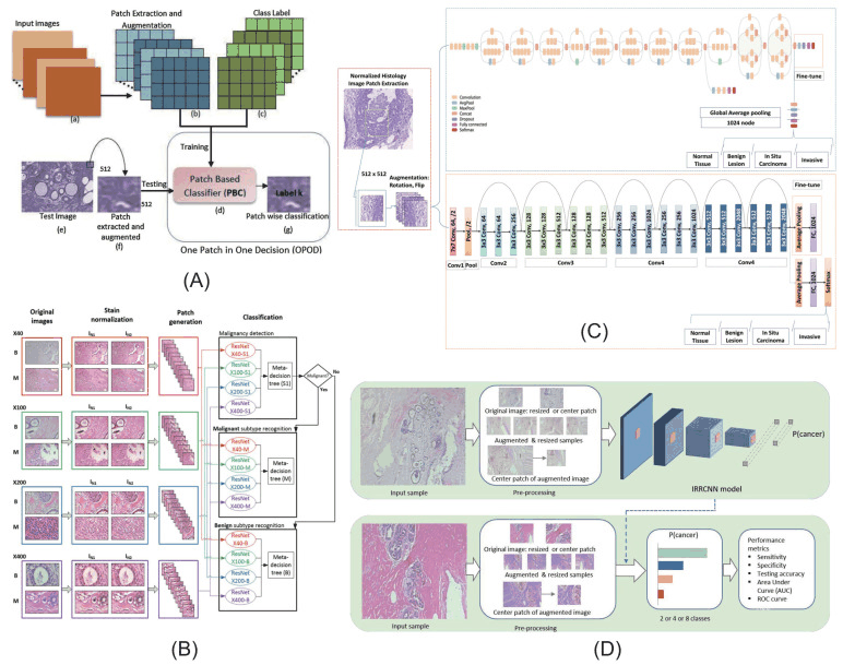
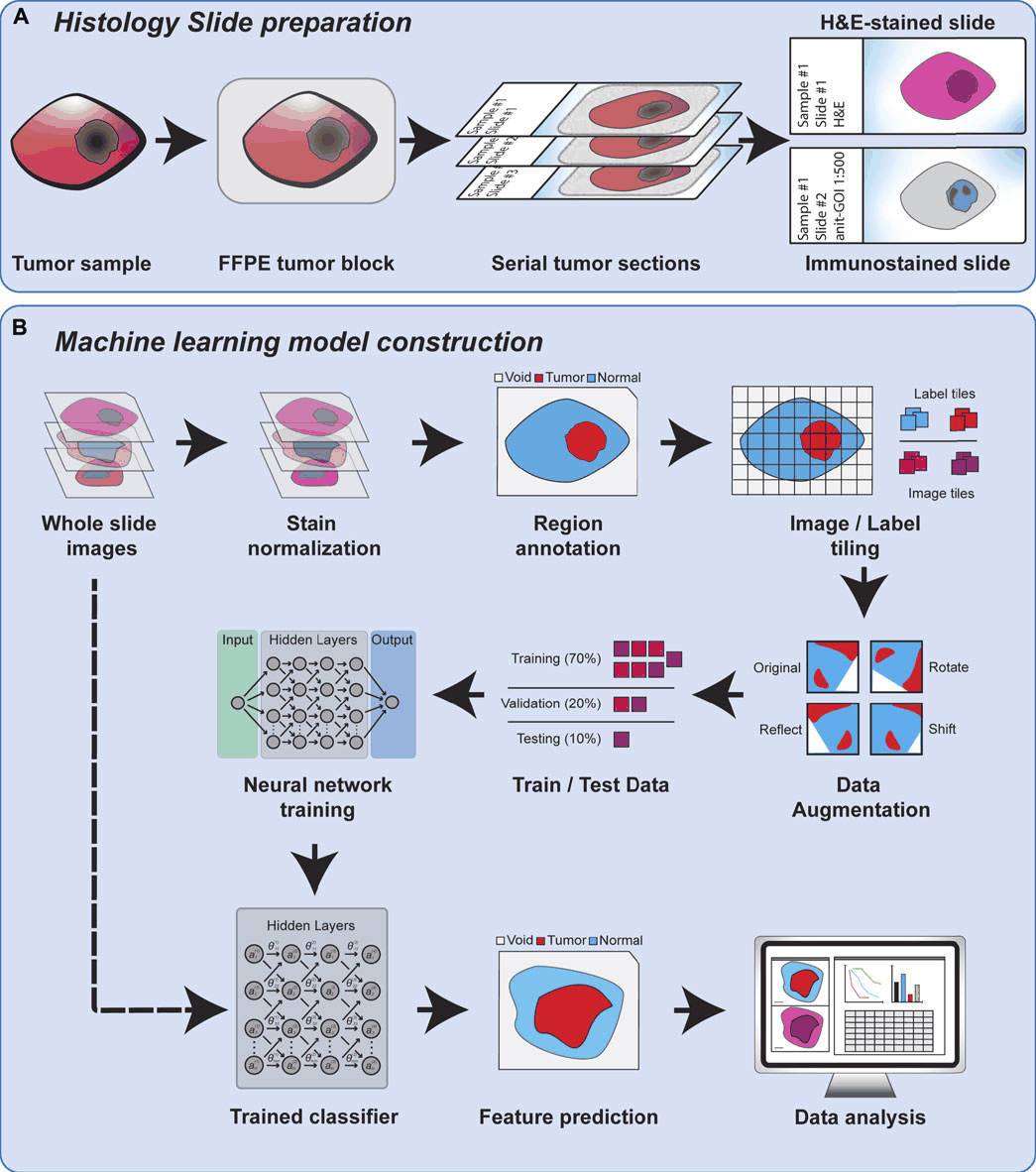
🧬 HistoAI — Cancer Histopathology AI Classifier Comparative Deep Learning with Spatial Attention for Histopathology Image Classification 📌 Overview HistoAI is a research-oriented deep learning framework for automated classification of cancer histopathology images. The project investigates and compares three ResNet-based approaches: Single-Task CNN — baseline image classification architecture. Multi-Task CNN — shared feature learning using a multi-task architecture. Spatial Attention Network — the proposed architecture incorporating spatial attention to emphasize informative regions within histopathology images. The framework provides an interactive Streamlit-based AI analysis dashboard for uploading histopathology specimens, comparing model predictions, visualizing confidence scores, and inspecting spatial attention responses. Research Prototype: This system is intended for research, educational, and demonstration purposes and is not designed to replace professional pathological diagnosis. 🎯 Research Objective The primary objective of this project is to investigate whether incorporating spatial attention mechanisms into a ResNet-based histopathology classifier can improve classification performance while providing more interpretable model behavior. The study compares conventional single-task learning against multi-task learning and the proposed spatial attention architecture. Research Question Can spatial attention improve histopathology image classification while providing interpretable spatial representations of the regions influencing model predictions? 🧠 Model Architecture The project evaluates three complementary architectures. 1. Single-Task CNN A conventional ResNet-based classifier trained directly for five-class histopathology classification. Input Image │ ▼ ResNet Backbone │ ▼ Feature Extraction │ ▼ Global Pooling │ ▼ Fully Connected Layer │ ▼ 5-Class Prediction
Comparative Deep Learning with Spatial Attention for Histopathology Image Classification
HistoAI is a research-oriented deep learning framework for automated classification of cancer histopathology images.
The framework provides an interactive Streamlit-based AI analysis dashboard for uploading histopathology specimens, comparing model predictions, visualizing confidence scores, and inspecting spatial attention responses.
Research Prototype: This system is intended for research, educational, and demonstration purposes and is not designed to replace professional pathological diagnosis.
4. Neural Network Backbone, Layer Specifications & Loss Formulations
The primary objective of this project is to investigate whether incorporating spatial attention mechanisms into a ResNet-based histopathology classifier can improve classification performance while providing more interpretable model behavior.
The study compares conventional single-task learning against multi-task learning and the proposed spatial attention architecture.
Can spatial attention improve histopathology image classification while providing interpretable spatial representations of the regions influencing model predictions?
A conventional ResNet-based classifier trained directly for five-class histopathology classification.
Input Image │ ▼ ResNet Backbone │ ▼ Feature Extraction │ ▼ Global Pooling │ ▼ Fully Connected Layer │ ▼ 5-Class Prediction
Cancer Histopathology AI Classifier — A comparative deep learning framework for histopathology image classification using Single-Task CNN, Multi-Task Learning, and a proposed Spatial Attention model with explainable attention visualization.
ChongQingNoSubway / DGR-MIL Star 154 Code for paper: DGR-MIL: Exploring Diverse Global Representation in Multiple Instance Learning for Whole Slide Image Classification [ECCV 2024] transformer weakly-supervised-learning whole-slide-imaging tumor-heterogeneity tumor-detection self-attention multiple-instance-learning tumor-classification histopathology histopathology-image-analysis Updated Dec 18, 2024 Python
Code for paper: DGR-MIL: Exploring Diverse Global Representation in Multiple Instance Learning for Whole Slide Image Classification [ECCV 2024]
open-pathology / awesome-pathology Star 139 Awesome List of Digital and Computational Pathology Resources awesome awesome-list digital-pathology pathology whole-slide-imaging computational-pathology heathcare histopathology histopathology-images histopathology-wsi histopathology-image-analysis Updated Feb 11, 2026
mkang315 / ASF-YOLO Star 118 [IMAVIS] Official implementation of "ASF-YOLO: A Novel YOLO Model with Attentional Scale Sequence Fusion for Cell Instance Segmentation". deep-neural-networks yolo medical-image-computing medical-image-processing cell-segmentation nucleus-detection computer-vision-algorithms instance-segmentation deep-learning-framework cell-detection medical-image-analysis data-science-bowl-2018 medical-image-segmentation nuclei-segmentation lesion-segmentation hematoxylin-eosin-staining breast-cancer-segmentation detection-segmentation-algorithm histopathology-image-analysis breast-cancer-cell Updated Sep 22, 2026 Python
[IMAVIS] Official implementation of "ASF-YOLO: A Novel YOLO Model with Attentional Scale Sequence Fusion for Cell Instance Segmentation".
ChongQingNoSubway / PDL Star 101 Code for the paper " PDL: Regularizing Multiple Instance Learning with Progressive Dropout Layers " weakly-supervised-learning whole-slide-imaging tumor-detection multiple-instance-learning histopathology histopathology-images whole-slide-image histopathology-image-analysis Updated Jul 11, 2024 Python
Code for the paper " PDL: Regularizing Multiple Instance Learning with Progressive Dropout Layers "
liupei101 / Pipeline-Processing-TCGA-Slides-for-MIL Star 98 This repo provides the pipeline of processing TCGA whole-slide images for downstream pathology analysis. tcga whole-slide-imaging multiple-instance-learning histopathology-image-analysis Updated Jun 23, 2026 Python
This repo provides the pipeline of processing TCGA whole-slide images for downstream pathology analysis.
Younger330 / SemanticEnergyLoss Star 30 BIBM2023 regular paper for "Addressing Sparse Annotation: a Novel Semantic Energy Loss for Tumor Cell Detection from Histopathologic Images" medical-imaging semi-supervised-learning weakly-supervised-learning pathology histopathology histopathology-images histopathology-image-analysis Updated May 12, 2025 Python
5. Training Protocol, Convergence Behavior & Experimental Evaluation
BIBM2023 regular paper for "Addressing Sparse Annotation: a Novel Semantic Energy Loss for Tumor Cell Detection from Histopathologic Images"
secrierlab / HistoMIL Star 30 A Python package for handling histopathology whole-slide images using multiple instance learning (MIL) techniques. deep-learning histopathology-image-analysis Updated May 21, 2024 Python
A Python package for handling histopathology whole-slide images using multiple instance learning (MIL) techniques.
HanaFEKI / Histopathology_foundation_models Star 17 A curated and practical guide to foundation models in computational pathology. This repo brings together key architectures, learning techniques, and PyTorch implementations, all in one place, to help researchers quickly understand, compare, and apply foundation models in histopathology and beyond. python pytorch-implementation huggingface-transformers foundation-models histopathology-image-analysis Updated Aug 28, 2025 Python
A curated and practical guide to foundation models in computational pathology. This repo brings together key architectures, learning techniques, and PyTorch implementations, all in one place, to help researchers quickly understand, compare, and apply foundation models in histopathology and beyond.
lely475 / SoftCTM Star 16 SoftCTM won 3rd place in the OCELOT 2023 Challenge. Multi-organ H&E-based deep learning model for cell detection, applicable for tumor cellularity/ purity/ content estimation. histology cell-detection histopathology tumor-purity-estimation histopathology-image-analysis tumor-cellularity-estimation Updated Oct 22, 2026 Python
SoftCTM won 3rd place in the OCELOT 2023 Challenge. Multi-organ H&E-based deep learning model for cell detection, applicable for tumor cellularity/ purity/ content estimation.
CedricCaruzzo / pannuke-segmentation Star 11 An open-source UNet-based pipeline for nuclei segmentation in histopathology images using the PanNuke dataset. It features an interactive web app for easy data visualization and handling, making AI tools accessible even for non-experts. This project provides a foundation for training and exploring histopathology data. python machine-learning deep-learning pytorch segmentation unet semantic-segmentation resnet-50 unet-pytorch unet-image-segmentation deeplab-v3-plus histopathology unet-segmentation resunet unetplusplus histopathology-image-analysis deeplab-v3-plus-pytorch Updated Jan 9, 2025 Python
An open-source UNet-based pipeline for nuclei segmentation in histopathology images using the PanNuke dataset. It features an interactive web app for easy data visualization and handling, making AI tools accessible even for non-experts. This project provides a foundation for training and exploring histopathology data.
DBO-DKFZ / multistain_cyclegan_normalization Star 11 Implementation of MultiStain-CycleGAN normalization cyclegan-pytorch stain histopathology-image-analysis Updated Jan 8, 2026 Python
PerceptionComputingLab / ULTRA Star 10 [MedIA2023 & MICCAI2022 ] Ambiguity-aware breast tumor cellularity estimation via self-ensemble label distribution learning label-distribution-learning brest-cancer-prediction histopathology-image-analysis neoadjuvant-treatment tumour-cellularity-estimation Updated Oct 9, 2023 Python
[MedIA2023 & MICCAI2022 ] Ambiguity-aware breast tumor cellularity estimation via self-ensemble label distribution learning
QuIIL / KBSMC_colon_cancer_grading_dataset Star 10 KBSMC colon cancer grading dataset repository colon-cancer cancer-grading histopathology-image-analysis Updated Jul 26, 2024 Python
BleeGleeWee / Histopathology-Image-Classification Star 10 Demonstration of potential in digital pathology applications from a CNN-based model to classify tumor vs normal histopathology image patches, applying transfer learning and Grad-CAM for interpretability. digital transfer-learning pathology cnn-for-visual-recognition gradcam histopathological-images gradcam-visualization histopathology-image-analysis Updated Dec 24, 2025 Jupyter Notebook
Demonstration of potential in digital pathology applications from a CNN-based model to classify tumor vs normal histopathology image patches, applying transfer learning and Grad-CAM for interpretability.
Zhengyushan / lagenet Star 8 The code for LAGE-Net wsi histopathology-images whole-slide-image histopathology-image-analysis histopathology-image-retrieval Updated Dec 2, 2021 Python
Model Figures & Evaluation Curves (4 Images)
Deep Learning Execution Pipeline
(Preprocessing)
(Feature Extraction)
(Self-Attention)
(Loss Optimization)