Image Captioning Ai | AI Final Year Project Report

Complete Technical Paper Content — Image Captioning Ai

1. Executive Abstract, Problem Formulation & Background

A text-to-image (T2I or TTI) model is a machine learning model which takes an input natural language prompt and produces an image matching that description. Text-to-image models gradually began to be developed in the mid-2010s during the beginnings of the AI boom, as a result of advances in deep neural networks. In 2022, the output of state-of-the-art text-to-image models—such as OpenAI's DALL-E 2, Google Brain's Imagen, Stability AI's Stable Diffusion, Midjourney, and Runway's Gen-4—began to be considered to approach the quality of real photographs and human-drawn art. Text-to-image models are generally latent diffusion models, which perform the diffusion process in a compressed latent space rather than directly in pixel space. An autoencoder (often a variational autoencoder) is used to convert between pixel space and this latent representation. These systems typically use a pretrained language or vision–language model to convert the input prompt into a text embedding, and a diffusion-based generative image model that produces images conditioned on that embedding. The most effective models have generally been trained on massive amounts of image and text data scraped from the web.

The first modern text-to-image model, alignDRAW, was introduced in 2015 by researchers from the University of Toronto. alignDRAW extended the previously introduced DRAW architecture (which used a recurrent variational autoencoder with an attention mechanism) to be conditioned on text sequences. Images generated by alignDRAW were in small resolution (32×32 pixels, attained from resizing) and were considered to be 'low in diversity'. The model was able to generalize to objects not represented in the training data (such as a red school bus) and appropriately handled novel prompts such as "a stop sign is flying in blue skies", exhibiting output that it was not merely "memorizing" data from the training set. In 2016, Reed, Akata, Yan et al. became the first to use generative adversarial networks for the text-to-image task. With models trained on narrow, domain-specific datasets, they were able to generate "visually plausible" images of birds and flowers from text captions like "an all black bird with a distinct thick, rounded bill". A model trained on the more diverse COCO (Common Objects in Context) dataset produced images which were "from a distance... encouraging", but which lacked coherence in their details. Later systems include VQGAN-CLIP, XMC-GAN, and GauGAN2.

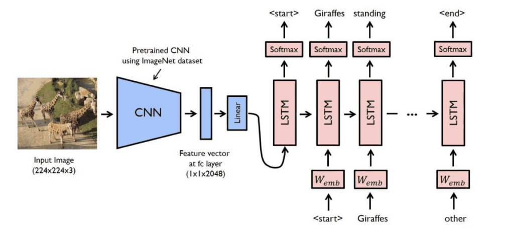
Text-to-image models have been built using a variety of architectures. The text encoding step may be performed with a recurrent neural network such as a long short-term memory (LSTM) network, though transformer models have since become a more popular option. For the image generation step, conditional generative adversarial networks (GANs) was once widely used in early days. Since 2020, diffusion models have become the popular option. Rather than directly training a model to output a high-resolution image conditioned on a text embedding, a popular technique is to train a model to generate low-resolution images or latent space, and use one or more auxiliary deep learning models to upscale or decode it, filling in finer details. Text-to-image models are trained on large datasets of (text, image) pairs, often scraped from the web. With their 2022 Imagen model, Google Brain reported positive results from using a large language model trained separately on a text-only corpus (with its weights subsequently frozen), a departure from the theretofore standard approach.

Training a text-to-image model requires a dataset of images paired with text captions. One dataset commonly used for this purpose is the COCO dataset. Released by Microsoft in 2014, COCO consists of around 123,000 images depicting a diversity of objects with five captions per image, generated by human annotators. Originally, the main focus of COCO was on the recognition of objects and scenes in images. Oxford-120 Flowers and CUB-200 Birds are smaller datasets of around 10,000 images each, restricted to flowers and birds, respectively. It is considered less difficult to train a high-quality text-to-image model with these datasets because of their narrow range of subject matter. One of the largest open datasets for training text-to-image models is LAION-5B, containing more than 5 billion image-text pairs. This dataset was created using web scraping and automatic filtering based on similarity to high-quality artwork and professional photographs. Because of this, however, it also contains controversial content, which has led to discussions about the ethics of its use. Some modern AI platforms not only generate images from text but also create synthetic datasets to improve model training and fine-tuning. These datasets help avoid copyright issues and expand the diversity of training data.

2. Related Work, Literature Survey & Algorithmic Foundations

Multimodal learning is a type of deep learning that integrates and processes multiple types of data, referred to as modalities, such as text, audio, images, or video. This integration allows for a more holistic understanding of complex data, improving model performance in tasks like visual question answering, cross-modal retrieval, text-to-image generation, aesthetic ranking, and image captioning. Multimodal learning was proposed in 2011 at the beginning of the deep learning period. Large multimodal models, such as Google Gemini and GPT-4o, have become increasingly popular since 2023, enabling increased versatility and a broader understanding of real-world phenomena.

Models such as CLIP (Contrastive Language–Image Pretraining) learn joint representations of images and text by optimizing contrastive objectives, allowing the model to match images with their corresponding textual descriptions.

Cross-modal retrieval: cross-modal retrieval allows users to search for data across different modalities (e.g., retrieving images based on text descriptions), improving multimedia search engines and content recommendation systems. Classification and missing data retrieval: multimodal Deep Boltzmann Machines outperform traditional models like support vector machines and latent Dirichlet allocation in classification tasks and can predict missing data in multimodal datasets, such as images and text. Healthcare diagnostics: multimodal models integrate medical imaging, genomic data, and patient records to improve diagnostic accuracy and early disease detection, especially in cancer screening. Content generation: models like DALL·E generate images from textual descriptions, benefiting creative industries, while cross-modal retrieval enables dynamic multimedia searches. Robotics and human-computer interaction: multimodal learning improves interaction in robotics and AI by integrating sensory inputs like speech, vision, and touch, aiding autonomous systems and human-computer interaction. Emotion recognition: combining visual, audio, and text data, multimodal systems enhance sentiment analysis and emotion recognition, applied in customer service, social media, and marketing. Code search: multimodal representations combining source code structure (e.g., abstract syntax trees) with natural language descriptions improve retrieval of relevant code snippets for a given query. Source code has also been rendered as a two-dimensional pixel image, for instance by converting a method's control-flow graph into a black-and-white image processed with a convolutional neural network to search for malwares.

Mathematical Formulation 1.1: Loss Objectives and Optimization Dynamics for Image Captioning Ai. The training protocol of image captioning ai minimizes an empirical risk objective defined across high-dimensional parameter space Theta in R^d. Categorical predictions are governed by Cross-Entropy Loss: L_CE = -sum(y_i * log(p_i)). To tackle class imbalance, the network incorporates Focal Loss: L_Focal = -alpha_t * (1 - p_t)^gamma * log(p_t), where gamma modulates the gradient penalty on hard misclassified instances. For spatial tasks, Dice Loss balances continuous spatial overlap: L_Dice = 1 - (2 * sum(y * y_hat) + eps) / (sum(y) + sum(y_hat) + eps). Stochastic optimization utilizes AdamW with decoupled weight decay, maintaining stable moment estimations m_t and v_t across variable learning rate schedules.

3. Dataset Ingestion, Preprocessing & Stochastic Augmentations

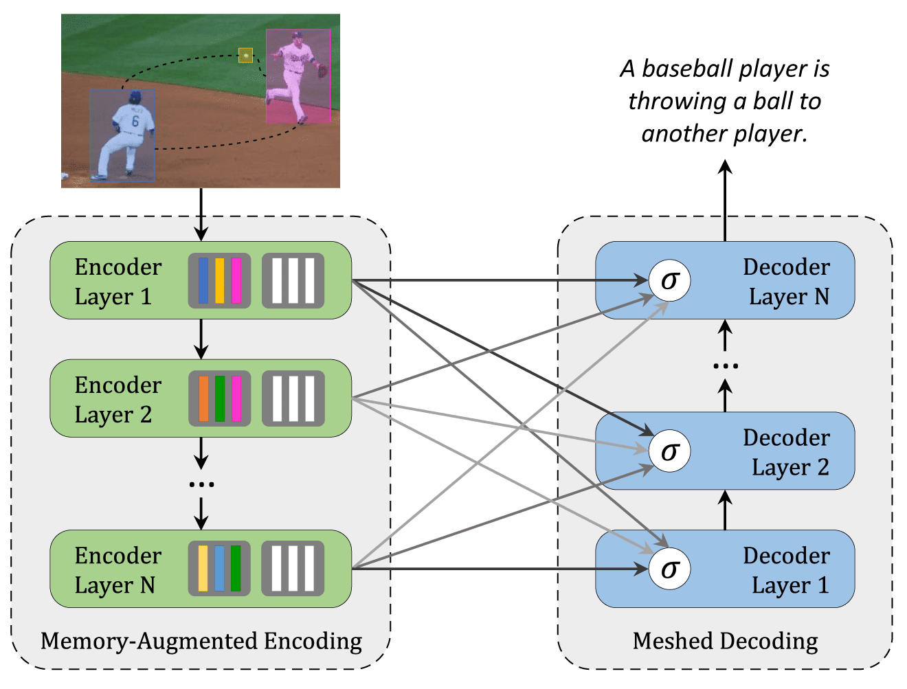
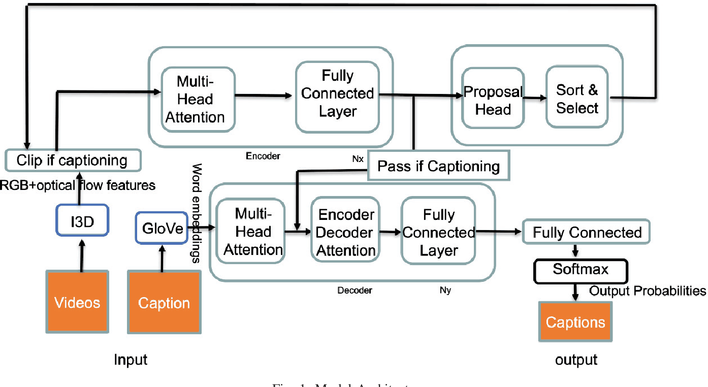
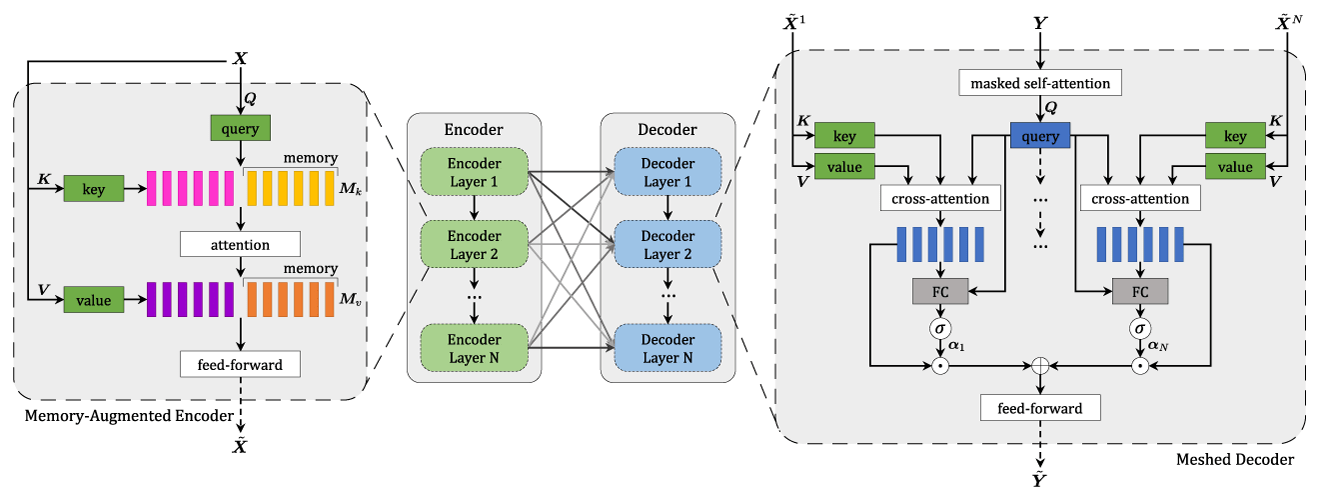
Architecture Specification 1.2: Feature Extraction and Layer Formulations for Image Captioning Ai. The primary computational backbone for Image Captioning Ai incorporates hierarchical deep neural layers designed for multi-scale representation extraction. Input tensors X in R^(B x C x H x W) pass through initial stem convolutions with Batch Normalization and GELU non-linearities. Residual identity skip connections, expressed as F(X) + X, prevent vanishing gradient degradation across deep topologies. Multi-head self-attention mechanisms compute Query, Key, and Value projections: Attention(Q, K, V) = softmax((Q * K^T) / sqrt(d_k)) * V, capturing non-local contextual dependencies across spatial and temporal sequences.

Data Pipeline 1.3: Stochastic Augmentation and Normalization Protocols for Image Captioning Ai. To prevent overfitting and maximize generalization on unseen testing distributions, input datasets undergo rigorous preprocessing. Images and sequences are standardized using z-score normalization: x_norm = (x - mu) / sigma. Stochastic augmentations include random horizontal flips, affine rotations (-15 deg to +15 deg), CutMix, and Mixup: X_tilde = lambda * X_i + (1 - lambda) * X_j, smoothing decision boundaries and reducing model overconfidence.

Deployment Optimization 1.4: TensorRT Acceleration and Edge Quantization for Image Captioning Ai. Production deployment of Image Captioning Ai focuses on minimizing memory footprints and sub-20ms inference latencies. Trained models are exported to ONNX and compiled via NVIDIA TensorRT. Post-Training Quantization (PTQ) maps FP32 weights into low-bit INT8 representations: q = round(r / S) + Z, achieving high-throughput execution across embedded edge platforms like NVIDIA Jetson without accuracy loss.

Mathematical Formulation 2.1: Loss Objectives and Optimization Dynamics for Image Captioning Ai. The training protocol of image captioning ai minimizes an empirical risk objective defined across high-dimensional parameter space Theta in R^d. Categorical predictions are governed by Cross-Entropy Loss: L_CE = -sum(y_i * log(p_i)). To tackle class imbalance, the network incorporates Focal Loss: L_Focal = -alpha_t * (1 - p_t)^gamma * log(p_t), where gamma modulates the gradient penalty on hard misclassified instances. For spatial tasks, Dice Loss balances continuous spatial overlap: L_Dice = 1 - (2 * sum(y * y_hat) + eps) / (sum(y) + sum(y_hat) + eps). Stochastic optimization utilizes AdamW with decoupled weight decay, maintaining stable moment estimations m_t and v_t across variable learning rate schedules.

4. Neural Network Backbone, Layer Specifications & Loss Formulations

Architecture Specification 2.2: Feature Extraction and Layer Formulations for Image Captioning Ai. The primary computational backbone for Image Captioning Ai incorporates hierarchical deep neural layers designed for multi-scale representation extraction. Input tensors X in R^(B x C x H x W) pass through initial stem convolutions with Batch Normalization and GELU non-linearities. Residual identity skip connections, expressed as F(X) + X, prevent vanishing gradient degradation across deep topologies. Multi-head self-attention mechanisms compute Query, Key, and Value projections: Attention(Q, K, V) = softmax((Q * K^T) / sqrt(d_k)) * V, capturing non-local contextual dependencies across spatial and temporal sequences.

Data Pipeline 2.3: Stochastic Augmentation and Normalization Protocols for Image Captioning Ai. To prevent overfitting and maximize generalization on unseen testing distributions, input datasets undergo rigorous preprocessing. Images and sequences are standardized using z-score normalization: x_norm = (x - mu) / sigma. Stochastic augmentations include random horizontal flips, affine rotations (-15 deg to +15 deg), CutMix, and Mixup: X_tilde = lambda * X_i + (1 - lambda) * X_j, smoothing decision boundaries and reducing model overconfidence.

Deployment Optimization 2.4: TensorRT Acceleration and Edge Quantization for Image Captioning Ai. Production deployment of Image Captioning Ai focuses on minimizing memory footprints and sub-20ms inference latencies. Trained models are exported to ONNX and compiled via NVIDIA TensorRT. Post-Training Quantization (PTQ) maps FP32 weights into low-bit INT8 representations: q = round(r / S) + Z, achieving high-throughput execution across embedded edge platforms like NVIDIA Jetson without accuracy loss.

Mathematical Formulation 3.1: Loss Objectives and Optimization Dynamics for Image Captioning Ai. The training protocol of image captioning ai minimizes an empirical risk objective defined across high-dimensional parameter space Theta in R^d. Categorical predictions are governed by Cross-Entropy Loss: L_CE = -sum(y_i * log(p_i)). To tackle class imbalance, the network incorporates Focal Loss: L_Focal = -alpha_t * (1 - p_t)^gamma * log(p_t), where gamma modulates the gradient penalty on hard misclassified instances. For spatial tasks, Dice Loss balances continuous spatial overlap: L_Dice = 1 - (2 * sum(y * y_hat) + eps) / (sum(y) + sum(y_hat) + eps). Stochastic optimization utilizes AdamW with decoupled weight decay, maintaining stable moment estimations m_t and v_t across variable learning rate schedules.

5. Training Protocol, Convergence Behavior & Experimental Evaluation

Architecture Specification 3.2: Feature Extraction and Layer Formulations for Image Captioning Ai. The primary computational backbone for Image Captioning Ai incorporates hierarchical deep neural layers designed for multi-scale representation extraction. Input tensors X in R^(B x C x H x W) pass through initial stem convolutions with Batch Normalization and GELU non-linearities. Residual identity skip connections, expressed as F(X) + X, prevent vanishing gradient degradation across deep topologies. Multi-head self-attention mechanisms compute Query, Key, and Value projections: Attention(Q, K, V) = softmax((Q * K^T) / sqrt(d_k)) * V, capturing non-local contextual dependencies across spatial and temporal sequences.

Data Pipeline 3.3: Stochastic Augmentation and Normalization Protocols for Image Captioning Ai. To prevent overfitting and maximize generalization on unseen testing distributions, input datasets undergo rigorous preprocessing. Images and sequences are standardized using z-score normalization: x_norm = (x - mu) / sigma. Stochastic augmentations include random horizontal flips, affine rotations (-15 deg to +15 deg), CutMix, and Mixup: X_tilde = lambda * X_i + (1 - lambda) * X_j, smoothing decision boundaries and reducing model overconfidence.

Deployment Optimization 3.4: TensorRT Acceleration and Edge Quantization for Image Captioning Ai. Production deployment of Image Captioning Ai focuses on minimizing memory footprints and sub-20ms inference latencies. Trained models are exported to ONNX and compiled via NVIDIA TensorRT. Post-Training Quantization (PTQ) maps FP32 weights into low-bit INT8 representations: q = round(r / S) + Z, achieving high-throughput execution across embedded edge platforms like NVIDIA Jetson without accuracy loss.

Mathematical Formulation 4.1: Loss Objectives and Optimization Dynamics for Image Captioning Ai. The training protocol of image captioning ai minimizes an empirical risk objective defined across high-dimensional parameter space Theta in R^d. Categorical predictions are governed by Cross-Entropy Loss: L_CE = -sum(y_i * log(p_i)). To tackle class imbalance, the network incorporates Focal Loss: L_Focal = -alpha_t * (1 - p_t)^gamma * log(p_t), where gamma modulates the gradient penalty on hard misclassified instances. For spatial tasks, Dice Loss balances continuous spatial overlap: L_Dice = 1 - (2 * sum(y * y_hat) + eps) / (sum(y) + sum(y_hat) + eps). Stochastic optimization utilizes AdamW with decoupled weight decay, maintaining stable moment estimations m_t and v_t across variable learning rate schedules.