Complete Technical Paper Content — Image Classification Ai
1. Executive Abstract, Problem Formulation & Background
In machine learning, reinforcement learning from human feedback (RLHF) is a technique to align an intelligent agent with human preferences. It involves training a reward model to represent preferences, which can then be used to train other models through reinforcement learning. In classical reinforcement learning, an intelligent agent's goal is to learn a function that guides its behavior, called a policy. The function is iteratively optimized to increase the reward signal derived from the agent's task performance. However, explicitly defining a reward function that accurately approximates human preferences is challenging. Therefore, RLHF seeks to train a "reward model" directly from human feedback. The reward model is first trained in a supervised manner to predict if a response to a given prompt is good (high reward) or bad (low reward) based on ranking data collected from human annotators. This model then serves as a reward function to improve an agent's policy through an optimization algorithm like proximal policy optimization. RLHF has applications in various domains in machine learning, including natural language processing tasks such as text summarization and conversational agents, computer vision tasks like text-to-image models, and the development of video game bots. While RLHF is an effective method of training models to act better in accordance with human preferences, it also faces challenges due to the way the human preference data is collected. Though RLHF does not require massive amounts of data to improve performance, sourcing high-quality preference data is still an expensive process. Furthermore, if the data is not carefully collected from a representative sample, the resulting model may exhibit unwanted biases.
where K {\displaystyle K} is the number of responses the labelers ranked, r θ ( x , y ) {\displaystyle r_{\theta }(x,y)} is the output of the reward model for prompt x {\displaystyle x} and completion y {\displaystyle y} , y w {\displaystyle y_{w}} is the preferred completion over y l {\displaystyle y_{l}} , σ ( x ) {\displaystyle \sigma (x)} denotes the sigmoid function, and E [ X ] {\displaystyle E[X]} denotes the expected value. This can be thought of as a form of logistic regression, where the model predicts the probability that a response y w {\displaystyle y_{w}} is preferred over y l {\displaystyle y_{l}} . This loss function essentially measures the difference between the reward model's predictions and the decisions made by humans. The goal is to make the model's guesses as close as possible to the humans' preferences by minimizing the difference measured by this equation. In the case of only pairwise comparisons, K = 2 {\displaystyle K=2} , so the factor of 1 / ( K 2 ) = 1 {\displaystyle 1/{\tbinom {K}{2}}=1} . In general, all ( K 2 ) {\displaystyle {\tbinom {K}{2}}} comparisons from each prompt are used for training as a single batch. After training, the outputs of the model are normalized such that the reference completions have a mean score of 0. That is, ∑ y r θ ( x , y ) = 0 {\textstyle \sum _{y}r_{\theta }(x,y)=0} for each query and reference pair ( x , y ) {\displaystyle (x,y)} by calculating the mean reward across the training dataset and setting it as the bias in the reward head.
The policy model is a function that takes a string as input, and produces another string. Usually in language modeling, the output string is not produced in one forward pass, but by multiple forward passes, generated autoregressively. Similarly to the reward model, the human feedback policy is also initialized from a pre-trained model. The key is to understand language generation as if it is a game to be learned by RL. In RL, a policy is a function that maps a game state to a game action. In RLHF, the "game" is the game of replying to prompts. A prompt and all previously generated tokens are the game state, and generating a new token is a game action. The first step in its training is supervised fine-tuning (SFT). This step does not require the reward model. Instead, the pre-trained model is trained on a dataset D S F T {\displaystyle D_{SFT}} that contains prompt-response pairs ( x , y ) {\displaystyle (x,y)} . Then, during SFT, the model is trained to auto-regressively generate the corresponding response y {\displaystyle y} when given a random prompt x {\displaystyle x} . The original paper recommends to SFT for only one epoch, since more than that causes overfitting. The dataset D S F T {\displaystyle D_{SFT}} is usually written by human contractors, who write both the prompts and responses. The second step uses a policy gradient method to the reward model. It uses a dataset D R L {\displaystyle D_{RL}} , which contains prompts, but not responses. Like most policy gradient methods, this algorithm has an outer loop and two inner loops:
Initialize the policy π ϕ R L {\displaystyle \pi _{\phi }^{RL}} to π S F T {\displaystyle \pi ^{SFT}} , the policy output from SFT. Loop for many steps. Initialize a new empty dataset D π ϕ R L {\displaystyle D_{\pi _{\phi }^{RL}}} . Loop for many steps Sample a random prompt x {\displaystyle x} from D R L {\displaystyle D_{RL}} . Generate a response y {\displaystyle y} from the policy π ϕ R L {\displaystyle \pi _{\phi }^{RL}} . Calculate the reward signal r θ ( x , y ) {\displaystyle r_{\theta }(x,y)} from the reward model r θ {\displaystyle r_{\theta }} . Add the triple ( x , y , r θ ( x , y ) ) {\displaystyle (x,y,r_{\theta }(x,y))} to D π ϕ R L {\displaystyle D_{\pi _{\phi }^{RL}}} . Update ϕ {\displaystyle \phi } by a policy gradient method to increase the objective function objective ( ϕ ) = E ( x , y ) ∼ D π ϕ RL [ r θ ( x , y ) − β log ( π ϕ RL ( y | x ) π SFT ( y | x ) ) ] {\displaystyle {\text{objective}}(\phi )=E_{(x,y)\sim D_{\pi _{\phi }^{\text{RL}}}}\left[r_{\theta }(x,y)-\beta \log \left({\frac {\pi _{\phi }^{\text{RL}}(y|x)}{\pi ^{\text{SFT}}(y|x)}}\right)\right]}
Note that ( x , y ) ∼ D π ϕ RL {\displaystyle (x,y)\sim D_{\pi _{\phi }^{\text{RL}}}} is equivalent to x ∼ D R L , y ∼ π ϕ RL ( ⋅ | x ) {\displaystyle x\sim D_{RL},y\sim \pi _{\phi }^{\text{RL}}(\cdot |x)} , which means "sample a prompt from D R L {\displaystyle D_{RL}} , then sample a response from the policy". The objective function has two parts. The first part is simply the expected reward E [ r ] {\displaystyle E[r]} , and is standard for any RL algorithm. The second part is a "penalty term" involving the KL divergence. The strength of the penalty term is determined by the hyperparameter β {\displaystyle \beta } . This KL term works by penalizing the KL divergence (a measure of statistical distance between distributions) between the model being fine-tuned and the initial supervised model. By choosing an appropriate β {\displaystyle \beta } , the training can balance learning from new data while retaining useful information from the initial model, increasing generalization by avoiding fitting too closely to the new data. Aside from preventing the new model from producing outputs too dissimilar those of the initial model, a second motivation of including the KL term is to encourage the model to output high-entropy text, so as to prevent the model from collapsing to a small number of canned responses. In simpler terms, the objective function calculates how well the policy's responses are expected to align with human feedback. The policy generates responses to prompts, and each response is evaluated both on how well it matches human preferences (as measured by the reward model) and how similar it is to responses the model would naturally generate. The goal is to balance improving alignment with human preferences while ensuring the model's responses remain diverse and not too far removed from what it has learned during its initial training. This helps the model not only to provide answers that people find useful or agreeable but also to maintain a broad understanding and avoid overly narrow or repetitive responses.
2. Related Work, Literature Survey & Algorithmic Foundations
The policy function is usually trained by proximal policy optimization (PPO) algorithm. That is, the parameter ϕ {\displaystyle \phi } is trained by gradient ascent on the clipped surrogate function. Classically, the PPO algorithm employs generalized advantage estimation, which means that there is an extra value estimator V ξ t ( x ) {\displaystyle V_{\xi _{t}}(x)} , that updates concurrently with the policy π ϕ t R L {\displaystyle \pi _{\phi _{t}}^{RL}} during PPO training: π ϕ t R L , V ξ t , π ϕ t + 1 R L , V ξ t + 1 , … {\displaystyle \pi _{\phi _{t}}^{RL},V_{\xi _{t}},\pi _{\phi _{t+1}}^{RL},V_{\xi _{t+1}},\dots } . The value estimator is used only during training, and not outside of training. The PPO uses gradient descent on the following clipped surrogate advantage: L PPO ( ϕ ) := E x ∼ D RL , y ∼ π ϕ t ( y | x ) [ min ( π ϕ R L ( y | x ) π ϕ t R L ( y | x ) A ( x , y ) , c l i p ( π ϕ R L ( y | x ) π ϕ t R L ( y | x ) , 1 − ϵ , 1 + ϵ ) A ( x , y ) ) ] {\displaystyle L_{\text{PPO}}(\phi ):=E_{x\sim D_{\text{RL}},y\sim \pi _{\phi _{t}}(y|x)}\left[\min \left({\frac {\pi _{\phi }^{RL}(y|x)}{\pi _{\phi _{t}}^{RL}(y|x)}}A(x,y),\mathrm {clip} \left({\frac {\pi _{\phi }^{RL}(y|x)}{\pi _{\phi _{t}}^{RL}(y|x)}},1-\epsilon ,1+\epsilon \right)A(x,y)\right)\right]}
where the advantage term A ( x , y ) {\displaystyle A(x,y)} is defined as r θ ( x , y ) − V ξ t ( x ) {\displaystyle r_{\theta }(x,y)-V_{\xi _{t}}(x)} . That is, the advantage is computed as the difference between the reward (the expected return) and the value estimation (the expected return from the policy). This is used to train the policy by gradient ascent on it, usually using a standard momentum-gradient optimizer, like the Adam optimizer. The original paper initialized the value estimator from the trained reward model. Since PPO is an actor-critic algorithm, the value estimator is updated concurrently with the policy, via minimizing the squared TD-error, which in this case equals the squared advantage term: L TD ( ξ ) = E ( x , y ) ∼ D π ϕ t RL [ ( r θ ( x , y ) − β log ( π ϕ t RL ( y | x ) π SFT ( y | x ) ) − V ξ ( x ) ) 2 ] {\displaystyle L_{\text{TD}}(\xi )=\mathbb {E} _{(x,y)\sim D{\pi _{\phi _{t}}^{\text{RL}}}}\left[\left(r_{\theta }(x,y)-\beta \log \left({\frac {\pi _{\phi _{t}}^{\text{RL}}(y|x)}{\pi ^{\text{SFT}}(y|x)}}\right)-V_{\xi }(x)\right)^{2}\right]} which is minimized by gradient descent on it. Other methods than squared TD-error might be used. See the actor-critic algorithm page for details.
L ( ϕ ) = E ( x , y ) ∼ D π ϕ RL [ r θ ( x , y ) − β log ( π ϕ RL ( y | x ) π SFT ( y | x ) ) ] + γ E x ∼ D pretrain [ log ( π ϕ RL ( x ) ) ] {\displaystyle L(\phi )=E_{(x,y)\sim D_{\pi _{\phi }^{\text{RL}}}}\left[r_{\theta }(x,y)-\beta \log \left({\frac {\pi _{\phi }^{\text{RL}}(y|x)}{\pi ^{\text{SFT}}(y|x)}}\right)\right]+\gamma E_{x\sim D_{\text{pretrain}}}[\log(\pi _{\phi }^{\text{RL}}(x))]}
where γ {\displaystyle \gamma } controls the strength of this pretraining term. This combined objective function is called PPO-ptx, where "ptx" means "Mixing Pretraining Gradients". It was first used in the InstructGPT paper. In total, this objective function defines the method for adjusting the RL policy, blending the aim of aligning with human feedback and maintaining the model's original language understanding. So, writing out fully explicitly, the PPO-ptx objective function is:
L PPO-ptx ( ϕ ) := E ( x , y ) ∼ D π ϕ t RL [ min ( π ϕ R L ( y | x ) π ϕ t R L ( y | x ) A ( x , y ) , c l i p ( π ϕ R L ( y | x ) π ϕ t R L ( y | x ) , 1 − ϵ , 1 + ϵ ) A ( x , y ) ) − β log ( π ϕ RL ( y | x ) π SFT ( y | x ) ) ] + γ E x ∼ D pretrain [ log ( π ϕ RL ( x ) ) ] {\displaystyle {\begin{aligned}L_{\text{PPO-ptx}}(\phi )&:=E_{(x,y)\sim D_{\pi _{\phi _{t}}^{\text{RL}}}}\left[\min \left({\frac {\pi _{\phi }^{RL}(y|x)}{\pi _{\phi _{t}}^{RL}(y|x)}}A(x,y),\mathrm {clip} \left({\frac {\pi _{\phi }^{RL}(y|x)}{\pi _{\phi _{t}}^{RL}(y|x)}},1-\epsilon ,1+\epsilon \right)A(x,y)\right)-\beta \log \left({\frac {\pi _{\phi }^{\text{RL}}(y|x)}{\pi ^{\text{SFT}}(y|x)}}\right)\right]\\&+\gamma E_{x\sim D_{\text{pretrain}}}[\log(\pi _{\phi }^{\text{RL}}(x))]\end{aligned}}}
3. Dataset Ingestion, Preprocessing & Stochastic Augmentations
We begin by gathering human preference dataset D {\displaystyle D} . We then fit a reward model r ∗ {\displaystyle r^{*}} to data, by maximum likelihood estimation using the Plackett–Luce model r ∗ = arg max r E ( x , y 1 , … , y N ) ∼ D [ ln ∏ k = 1 N e r ( x , y k ) ∑ i = k N e r ( x , y i ) ] {\displaystyle r^{*}=\arg \max _{r}\mathbb {E} _{(x,y_{1},\dots ,y_{N})\sim D}\left[\ln \prod _{k=1}^{N}{\frac {e^{r(x,y_{k})}}{\sum _{i=k}^{N}e^{r(x,y_{i})}}}\right]}
We finally train an optimal policy π ∗ {\displaystyle \pi ^{*}} that maximizes the objective function: π ∗ = arg max π RL E ( x , y ) ∼ D π RL [ r ∗ ( x , y ) − β log ( π RL ( y | x ) π SFT ( y | x ) ) ] {\displaystyle \pi ^{*}=\arg \max _{\pi ^{\text{RL}}}\mathbb {E} _{(x,y)\sim D_{\pi ^{\text{RL}}}}\left[r^{*}(x,y)-\beta \log \left({\frac {\pi ^{\text{RL}}(y|x)}{\pi ^{\text{SFT}}(y|x)}}\right)\right]}
However, instead of doing the intermediate step of the reward model, DPO directly optimizes for the final policy. First, solve directly for the optimal policy, which can be done by Lagrange multipliers, as usual in statistical mechanics: π ∗ ( y | x ) = π SFT ( y | x ) exp ( r ∗ ( x , y ) / β ) Z ( x ) , {\displaystyle \pi ^{*}(y|x)={\frac {\pi ^{\text{SFT}}(y|x)\exp(r^{*}(x,y)/\beta )}{Z(x)}},}
where Z ( x ) {\displaystyle Z(x)} is the partition function. This is unfortunately not tractable, since it requires summing over all possible responses: Z ( x ) = ∑ y π SFT ( y | x ) exp ( r ∗ ( x , y ) / β ) = E y ∼ π SFT ( ⋅ | x ) [ exp ( r ∗ ( x , y ) / β ) ] {\displaystyle Z(x)=\sum _{y}\pi ^{\text{SFT}}(y|x)\exp(r^{*}(x,y)/\beta )=\mathbb {E} _{y\sim \pi ^{\text{SFT}}(\cdot |x)}[\exp(r^{*}(x,y)/\beta )]}
Next, invert this relationship to express the reward implicitly in terms of the optimal policy: r ∗ ( x , y ) = β log π ∗ ( y | x ) π SFT ( y | x ) + β log Z ( x ) . {\displaystyle r^{*}(x,y)=\beta \log {\frac {\pi ^{*}(y|x)}{\pi ^{\text{SFT}}(y|x)}}+\beta \log Z(x).}
4. Neural Network Backbone, Layer Specifications & Loss Formulations
Finally, plug it back to the maximum likelihood estimator, we obtain π ∗ = arg max π E ( x , y 1 , … , y N ) ∼ D [ ln ∏ k = 1 N e β log π ( y k | x ) π SFT ( y k | x ) ∑ i = k N e β log π ( y i | x ) π SFT ( y i | x ) ] {\displaystyle \pi ^{*}=\arg \max _{\pi }\mathbb {E} _{(x,y_{1},\dots ,y_{N})\sim D}\left[\ln \prod _{k=1}^{N}{\frac {e^{\beta \log {\frac {\pi (y_{k}|x)}{\pi ^{\text{SFT}}(y_{k}|x)}}}}{\sum _{i=k}^{N}e^{\beta \log {\frac {\pi (y_{i}|x)}{\pi ^{\text{SFT}}(y_{i}|x)}}}}}\right]}
Usually, DPO is used for modeling human preference in pairwise comparisons, so that N = 2 {\displaystyle N=2} . In that case, we have π ∗ = arg max π E ( x , y w , y l ) ∼ D [ log σ ( β log π ( y w | x ) π SFT ( y w | x ) − β log π ( y l | x ) π SFT ( y l | x ) ) ] {\displaystyle \pi ^{*}=\arg \max _{\pi }\mathbb {E} _{(x,y_{w},y_{l})\sim D}\left[\log \sigma \left(\beta \log {\frac {\pi (y_{w}|x)}{\pi ^{\text{SFT}}(y_{w}|x)}}-\beta \log {\frac {\pi (y_{l}|x)}{\pi ^{\text{SFT}}(y_{l}|x)}}\right)\right]}
DPO eliminates the need for a separate reward model or reinforcement learning loop, treating alignment as a supervised learning problem over preference data. This is simpler to implement and train than RLHF and has been shown to produce comparable and sometimes superior results. Nevertheless, RLHF has also been shown to beat DPO on some datasets, for example, on benchmarks that attempt to measure truthfulness. Therefore, the choice of method may vary depending on the features of the human preference data and the nature of the task. Like most preference-learning methods, DPO does not directly minimize the ranking error—how often the model scores the rejected response above the preferred one, but a smoother proxy ("surrogate") loss that is easier to optimize. Mohri and Zhong (2026) showed that for model classes that can assign nearly equal scores to two responses, as neural networks can, lowering this proxy loss does not guarantee that the ranking error falls: a model can bring the DPO loss essentially as low as any model in its class can by making its two scores nearly equal, without learning which response is better (in technical terms, the loss is not H-consistent). They showed that requiring a minimum gap, or margin, between the two scores restores the guarantee, and proposed structure-aware DPO (SA-DPO), which demands a larger gap when the two responses differ substantially in meaning and a smaller one when they are near-synonyms. They reported that SA-DPO outperformed DPO in their experiments.
v ( x , y ) = { λ D σ ( β ( r θ ( x , y ) − z 0 ) ) , if y ∼ y d e s i r a b l e ∣ x , λ U σ ( β ( z 0 − r θ ( x , y ) ) ) , if y ∼ y u n d e s i r a b l e ∣ x {\displaystyle v(x,y)\;=\;{\begin{cases}\lambda _{D}\,\sigma \!{\bigl (}\,\beta \,{\bigl (}r_{\theta }(x,y)\;-\;z_{0}{\bigr )}{\bigr )},&\quad {\text{if }}y\sim y_{\mathrm {desirable} \mid x},\\[6pt]\lambda _{U}\,\sigma \!{\bigl (}\,\beta \,{\bigl (}z_{0}\;-\;r_{\theta }(x,y){\bigr )}{\bigr )},&\quad {\text{if }}y\sim y_{\mathrm {undesirable} \mid x}\end{cases}}}
Here, β {\displaystyle \beta } controls how “risk-averse” the value function is (larger β {\displaystyle \beta } = faster saturation in the logistic function σ {\displaystyle \sigma } )and z 0 = K L ( π θ ( y ′ ∣ x ) ‖ π r e f ( y ′ ∣ x ) ) {\textstyle z_{0}=\mathrm {KL} \!{\Bigl (}\,\pi _{\theta }(y'\mid x)\;{\big \Vert }\;\pi _{\mathrm {ref} }(y'\mid x){\Bigr )}} is a baseline given by the Kullback–Leibler divergence. Since many real-world feedback pipelines yield "like/dislike" data more easily than pairwise comparisons, KTO is designed to be data-efficient and to reflect "loss aversion" more directly by using a straightforward notion of "good vs. bad" at the example level.
5. Training Protocol, Convergence Behavior & Experimental Evaluation
Machine learning (ML) is a field of study in artificial intelligence concerned with the development and study of statistical algorithms that can learn from data and generalize to unseen data, and thus perform tasks without being explicitly programmed. Statistics and mathematical optimisation methods compose the foundations of machine learning. Data mining is a related field of study, focusing on exploratory data analysis (EDA) through unsupervised learning. From a theoretical viewpoint, probably approximately correct learning provides a mathematical and statistical framework for describing machine learning. Most traditional machine learning and deep learning algorithms can be described as empirical risk minimisation under this framework. Advances in the field of deep learning have allowed neural networks, a class of statistical algorithms, to surpass many previous machine learning approaches in performance. The resulting dominance of machine learning within the field of AI from the late 2000s and early 2010s onwards was such that the terms "machine learning" and "artificial intelligence" are now often used interchangeably, even though they are not synonymous.
The term machine learning was coined in 1959 by Arthur Samuel, an IBM employee and pioneer in the field of computer gaming and artificial intelligence. The synonym self-teaching computers was also used during this time period. The earliest machine learning program was introduced in the 1950s, when Samuel invented a computer program that calculated the chance of winning in checkers for each side, but the history of machine learning is rooted in decades of efforts to study human cognitive processes. In 1949, Canadian psychologist Donald Hebb published the book The Organization of Behavior, in which he introduced a theoretical neural structure formed by certain interactions among nerve cells. The Hebbian theory of neuron interaction set the groundwork for how many machine learning algorithms work, with connected artificial neurons changing the strength of their connections based on data. Other researchers who have studied human cognitive systems contributed to the modern machine learning technologies as well, including Walter Pitts and Warren McCulloch, who proposed the first mathematical model of neural networks including algorithms that mirror human thought processes. By the early 1960s, an experimental "learning machine" with punched tape memory, called Cybertron, had been developed by Raytheon Company to analyse sonar signals, electrocardiograms, and speech patterns using rudimentary reinforcement learning. It was repetitively "trained" by a human operator/teacher to recognise patterns and equipped with a "goof" button to cause it to reevaluate incorrect decisions. A representative book on research into machine learning during the 1960s was Nils Nilsson's book "Learning Machines", dealing mostly with machine learning for pattern classification. Interest related to pattern recognition continued into the 1970s, as described by Duda and Hart in 1973. In 1981, a report was given on using teaching strategies so that an artificial neural network learns to recognise 40 characters (26 letters, 10 digits, and 4 special symbols) from a computer terminal. Tom M. Mitchell provided a widely quoted, more formal definition of the algorithms studied in the machine learning field: "A computer program is said to learn from experience E with respect to some class of tasks T and performance measure P if its performance at tasks in T, as measured by P, improves with experience E." This definition of the tasks in which machine learning is concerned is fundamentally operational rather than defining the field in cognitive terms. This follows Alan Turing's proposal in his paper "Computing Machinery and Intelligence", in which the question, "Can machines think?", is replaced by asking whether machines can convincingly imitate a human in its responses to human-posed questions. In 2012, AlexNet, developed by Alex Krizhevsky, Ilya Sutskever, and Geoffrey Hinton, achieved substantially improved results in the ImageNet image recognition competition, contributing to the wider adoption of deep neural networks. In 2013, Tomáš Mikolov and colleagues introduced word2vec, techniques for efficiently learning distributed vector representations of words from large text corpora. In 2014, Ian Goodfellow and colleagues introduced generative adversarial networks (GANs), a framework for training generative models through an adversarial process. In 2016, AlphaGo became the first computer program to defeat a professional human Go player without handicaps on a full-sized board, using deep neural networks and reinforcement learning. In 2017, Ashish Vaswani and colleagues introduced the Transformer, a neural network architecture based primarily on attention rather than recurrence or convolution.
As a scientific endeavour, machine learning grew out of the quest for artificial intelligence (AI). In the early days of AI as an academic discipline, some researchers were interested in having machines learn from data. They attempted to approach the problem with various symbolic methods, as well as what were then termed "neural networks"; these were mostly perceptrons and other models that were later found to be reinventions of the generalised linear models of statistics. Probabilistic reasoning was also employed, especially in automated medical diagnosis. However, an increasing emphasis on the logical, knowledge-based approach caused a rift between AI and machine learning. Probabilistic systems were plagued by theoretical and practical problems of data acquisition and representation. By 1980, expert systems had come to dominate AI, and statistics was out of favour. Work on symbolic/knowledge-based learning continued within AI, leading to inductive logic programming (ILP), but the more statistical line of research was now outside the field of AI proper, in pattern recognition and information retrieval. Neural network research was abandoned by AI and computer science around the same time. This subfield, termed "connectionism", was continued by researchers from other disciplines, including John Hopfield, David Rumelhart, and Geoffrey Hinton. Their main success came in the mid-1980s with the reinvention of backpropagation. Machine learning (ML), reorganised and recognised as its own field, started to flourish in the 1990s. The field changed its goal from achieving artificial intelligence to tackling solvable problems of a practical nature. It shifted focus away from the symbolic approaches it had inherited from AI, and toward methods and models borrowed from statistics, fuzzy logic, and probability theory.
A core objective of a learner is to generalise from its experience. Generalisation in this context is the ability of a learning machine to perform accurately on new, unseen examples/tasks after having experienced a learning data set. The training examples come from some generally unknown probability distribution (considered representative of the space of occurrences) and the learner has to build a general model about this space that enables it to produce sufficiently accurate predictions in new cases. The computational analysis of machine learning algorithms and their performance is a branch of theoretical computer science known as computational learning theory. One major framework is the probably approximately correct learning model. Because training sets are finite and the future is uncertain, learning theory usually does not yield guarantees of the performance of algorithms. Instead, probabilistic bounds on the performance are quite common. The bias–variance decomposition is one way to quantify generalisation error. For the best performance in the context of generalisation, the complexity of the hypothesis should match the complexity of the function underlying the data. If the hypothesis is less complex than the function, then the model has underfitted the data. If the complexity of the model is increased in response, then the training error decreases. But if the hypothesis is too complex, then the model is subject to overfitting and generalisation will be poorer. In addition to performance bounds, learning theorists study the time complexity and feasibility of learning. In computational learning theory, a computation is considered feasible if it can be done in polynomial time. There are two kinds of time complexity results: Positive results show that a certain class of functions can be learned in polynomial time. Negative results show that certain classes cannot be learned in polynomial time.
Machine learning approaches are traditionally divided into three broad categories, which correspond to learning paradigms, depending on the nature of the "signal" or "feedback" available to the learning system:
Model Figures & Evaluation Curves (4 Images)
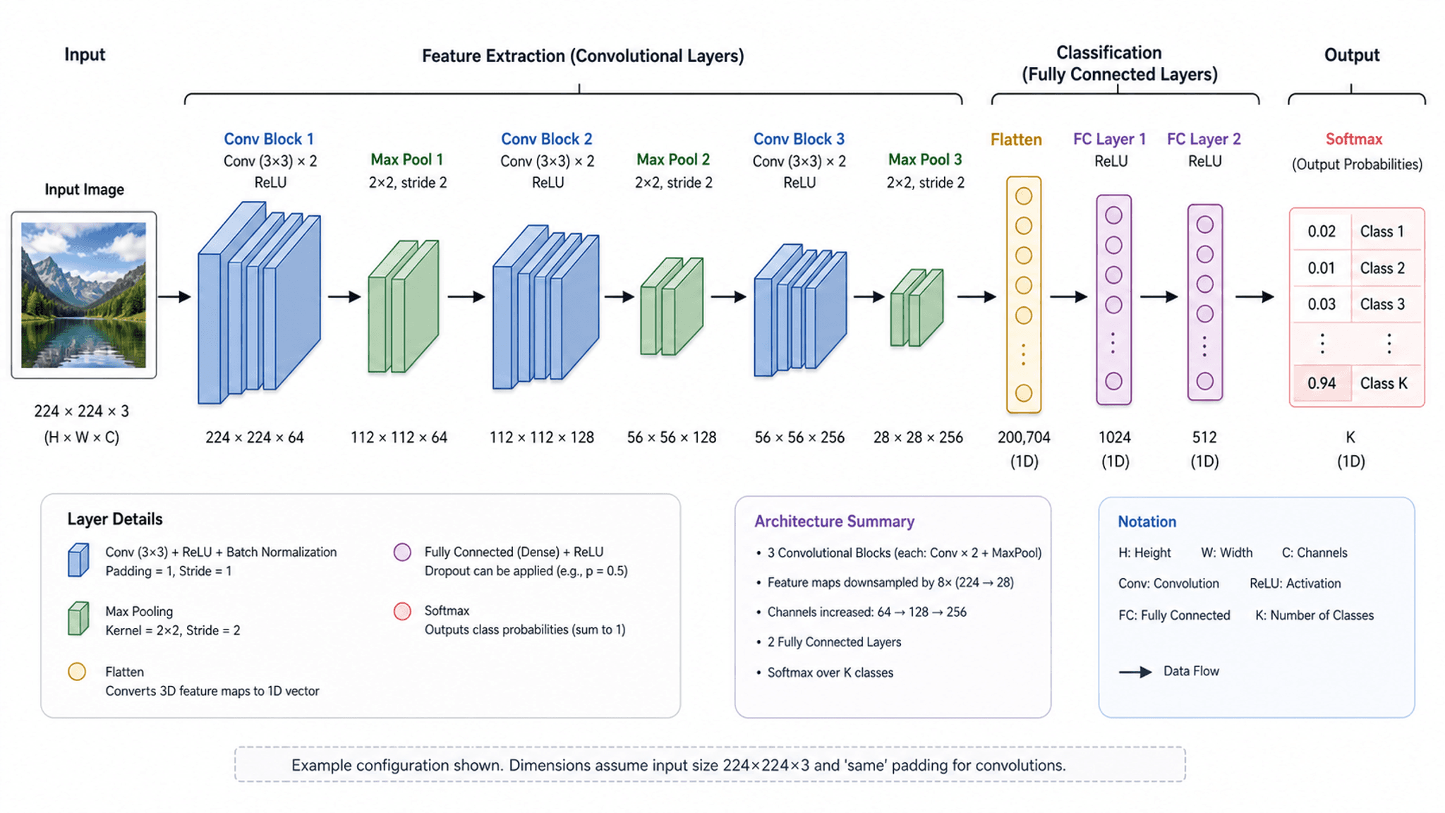
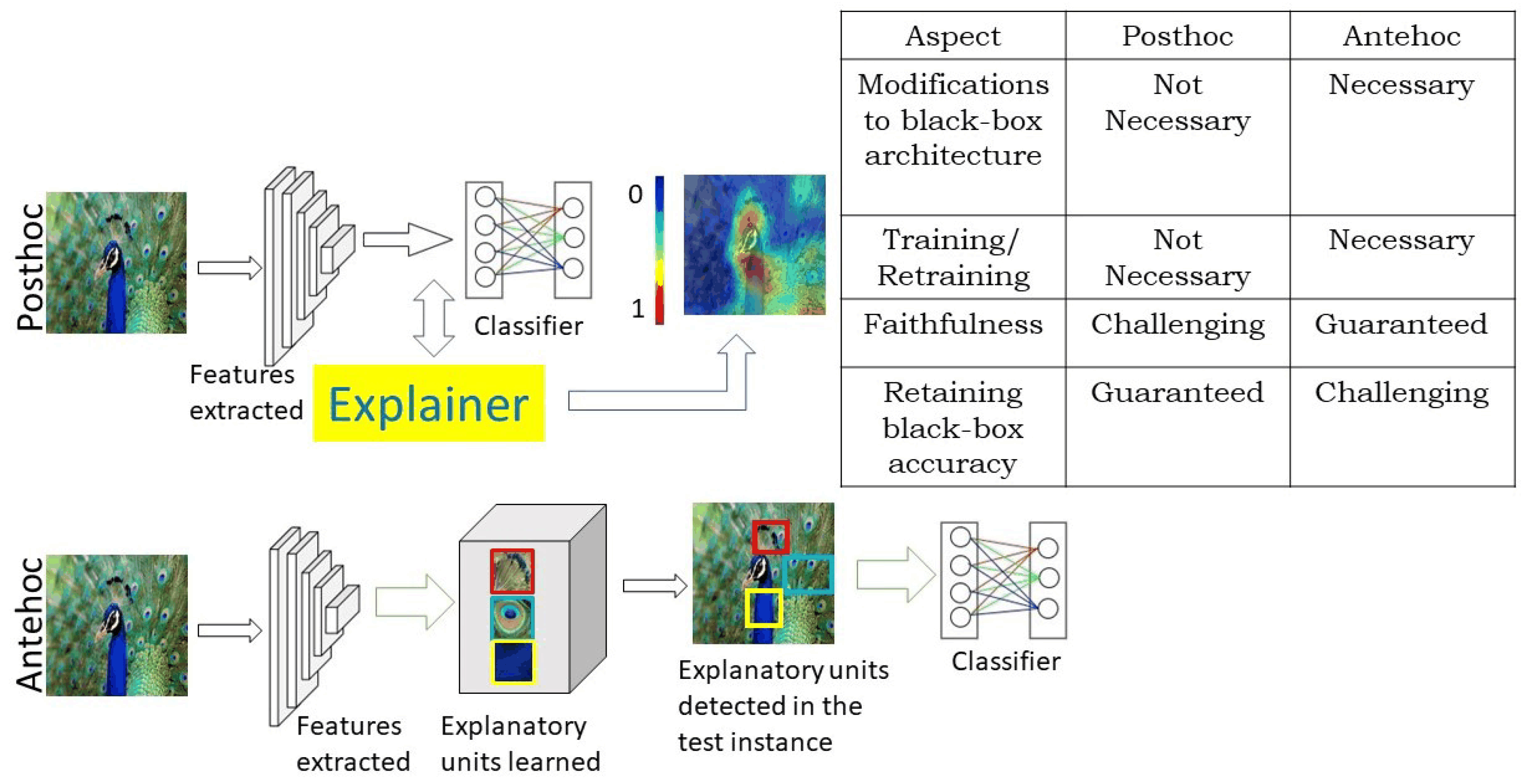
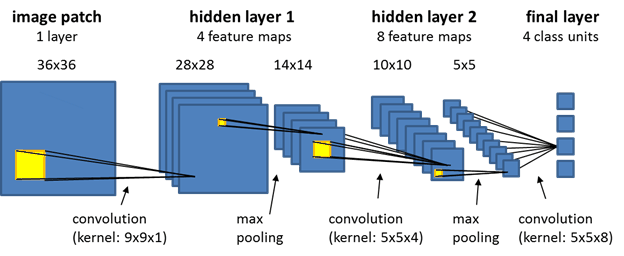
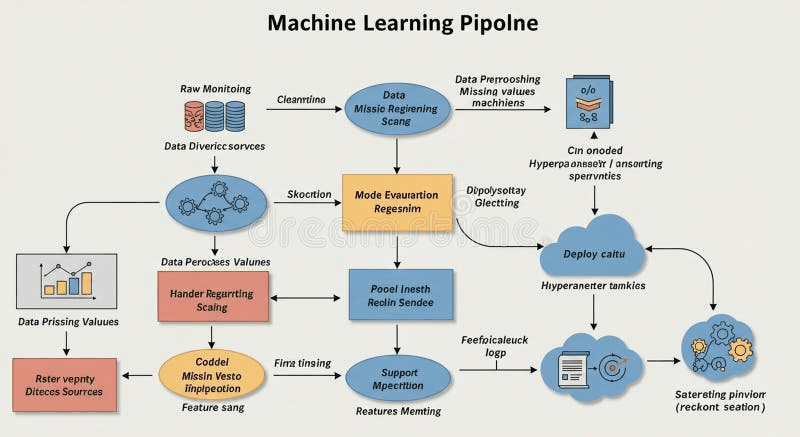
Deep Learning Execution Pipeline
(Preprocessing)
(Feature Extraction)
(Self-Attention)
(Loss Optimization)