Complete Technical Paper Content — Lifelong Learning Ai
1. Executive Abstract, Problem Formulation & Background
In computer science, online machine learning is a method of machine learning in which data becomes available in a sequential order and is used to update the best predictor for future data at each step, as opposed to batch learning techniques which generate the best predictor by learning on the entire training data set at once. Online learning is a common technique used in areas of machine learning where it is computationally infeasible to train over the entire dataset, requiring the need of out-of-core algorithms. It is also used in situations where it is necessary for the algorithm to dynamically adapt to new patterns in the data, or when the data itself is generated as a function of time, e.g., prediction of prices in the financial international markets. Online learning algorithms may be prone to catastrophic interference, a problem that can be addressed by incremental learning approaches. Online machine learning algorithms find applications in a wide variety of fields such as sponsored search to maximize ad revenue, portfolio optimization, shortest path prediction (with stochastic weights, e.g. traffic on roads for a maps application), spam filtering, real-time fraud detection, dynamic pricing for e-commerce, etc. There is also growing interest in usage of online learning paradigms for LLMs to enable continuous, real-time adaptation after the initial training.
I [ f ] = E [ V ( f ( x ) , y ) ] = ∫ V ( f ( x ) , y ) d p ( x , y ) . {\displaystyle I[f]=\mathbb {E} [V(f(x),y)]=\int V(f(x),y)\,dp(x,y)\ .}
A common paradigm in this situation is to estimate a function f ^ {\displaystyle {\hat {f}}} through empirical risk minimization or regularized empirical risk minimization (usually Tikhonov regularization). The choice of loss function here gives rise to several well-known learning algorithms such as regularized least squares and support vector machines. A purely online model in this category would learn based on just the new input ( x t + 1 , y t + 1 ) {\displaystyle (x_{t+1},y_{t+1})} , the current best predictor f t {\displaystyle f_{t}} and some extra stored information (which is usually expected to have storage requirements independent of training data size). For many formulations, for example nonlinear kernel methods, true online learning is not possible, though a form of hybrid online learning with recursive algorithms can be used where f t + 1 {\displaystyle f_{t+1}} is permitted to depend on f t {\displaystyle f_{t}} and all previous data points ( x 1 , y 1 ) , … , ( x t , y t ) {\displaystyle (x_{1},y_{1}),\ldots ,(x_{t},y_{t})} . In this case, the space requirements are no longer guaranteed to be constant since it requires storing all previous data points, but the solution may take less time to compute with the addition of a new data point, as compared to batch learning techniques. A common strategy to overcome the above issues is to learn using mini-batches, which process a small batch of b ≥ 1 {\displaystyle b\geq 1} data points at a time, this can be considered as pseudo-online learning for b {\displaystyle b} much smaller than the total number of training points. Mini-batch techniques are used with repeated passing over the training data to obtain optimized out-of-core versions of machine learning algorithms, for example, stochastic gradient descent. When combined with backpropagation, this is currently the de facto training method for training artificial neural networks.
The simple example of linear least squares is used to explain a variety of ideas in online learning. The ideas are general enough to be applied to other settings, for example, with other convex loss functions.
f ( x j ) = ⟨ w , x j ⟩ = w ⋅ x j {\displaystyle f(x_{j})=\langle w,x_{j}\rangle =w\cdot x_{j}}
where x j ∈ R d {\displaystyle x_{j}\in \mathbb {R} ^{d}} is a vector of inputs (data points) and w ∈ R d {\displaystyle w\in \mathbb {R} ^{d}} is a linear filter vector. The goal is to compute the filter vector w {\displaystyle w} . To this end, a square loss function
V ( f ( x j ) , y j ) = ( f ( x j ) − y j ) 2 = ( ⟨ w , x j ⟩ − y j ) 2 {\displaystyle V(f(x_{j}),y_{j})=(f(x_{j})-y_{j})^{2}=(\langle w,x_{j}\rangle -y_{j})^{2}}
is used to compute the vector w {\displaystyle w} that minimizes the empirical loss
I n [ w ] = ∑ j = 1 n V ( ⟨ w , x j ⟩ , y j ) = ∑ j = 1 n ( x j T w − y j ) 2 {\displaystyle I_{n}[w]=\sum _{j=1}^{n}V(\langle w,x_{j}\rangle ,y_{j})=\sum _{j=1}^{n}(x_{j}^{\mathsf {T}}w-y_{j})^{2}} where
y j ∈ R . {\displaystyle y_{j}\in \mathbb {R} .}
Let X {\displaystyle X} be the i × d {\displaystyle i\times d} data matrix and y ∈ R i {\displaystyle y\in \mathbb {R} ^{i}} is the column vector of target values after the arrival of the first i {\displaystyle i} data points. Assuming that the covariance matrix Σ i = X T X {\displaystyle \Sigma _{i}=X^{\mathsf {T}}X} is invertible (otherwise it is preferential to proceed in a similar fashion with Tikhonov regularization), the best solution f ∗ ( x ) = ⟨ w ∗ , x ⟩ {\displaystyle f^{*}(x)=\langle w^{*},x\rangle } to the linear least squares problem is given by
w ∗ = ( X T X ) − 1 X T y = Σ i − 1 ∑ j = 1 i x j y j . {\displaystyle w^{*}=(X^{\mathsf {T}}X)^{-1}X^{\mathsf {T}}y=\Sigma _{i}^{-1}\sum _{j=1}^{i}x_{j}y_{j}.}
2. Related Work, Literature Survey & Algorithmic Foundations
Now, calculating the covariance matrix Σ i = ∑ j = 1 i x j x j T {\displaystyle \Sigma _{i}=\sum _{j=1}^{i}x_{j}x_{j}^{\mathsf {T}}} takes time O ( i d 2 ) {\displaystyle O(id^{2})} , inverting the d × d {\displaystyle d\times d} matrix takes time O ( d 3 ) {\displaystyle O(d^{3})} , while the rest of the multiplication takes time O ( d 2 ) {\displaystyle O(d^{2})} , giving a total time of O ( i d 2 + d 3 ) {\displaystyle O(id^{2}+d^{3})} . When there are n {\displaystyle n} total points in the dataset, to recompute the solution after the arrival of every datapoint i = 1 , … , n {\displaystyle i=1,\ldots ,n} , the naive approach will have a total complexity O ( n 2 d 2 + n d 3 ) {\displaystyle O(n^{2}d^{2}+nd^{3})} . Note that when storing the matrix Σ i {\displaystyle \Sigma _{i}} , then updating it at each step needs only adding x i + 1 x i + 1 T {\displaystyle x_{i+1}x_{i+1}^{\mathsf {T}}} , which takes O ( d 2 ) {\displaystyle O(d^{2})} time, reducing the total time to O ( n d 2 + n d 3 ) = O ( n d 3 ) {\displaystyle O(nd^{2}+nd^{3})=O(nd^{3})} , but with an additional storage space of O ( d 2 ) {\displaystyle O(d^{2})} to store Σ i {\displaystyle \Sigma _{i}} .
Γ i = Γ i − 1 − Γ i − 1 x i x i T Γ i − 1 1 + x i T Γ i − 1 x i {\displaystyle \Gamma _{i}=\Gamma _{i-1}-{\frac {\Gamma _{i-1}x_{i}x_{i}^{\mathsf {T}}\Gamma _{i-1}}{1+x_{i}^{\mathsf {T}}\Gamma _{i-1}x_{i}}}}
w i = w i − 1 − Γ i x i ( x i T w i − 1 − y i ) {\displaystyle w_{i}=w_{i-1}-\Gamma _{i}x_{i}\left(x_{i}^{\mathsf {T}}w_{i-1}-y_{i}\right)}
The above iteration algorithm can be proved using induction on i {\displaystyle i} . The proof also shows that Γ i = Σ i − 1 {\displaystyle \Gamma _{i}=\Sigma _{i}^{-1}} . One can look at RLS also in the context of adaptive filters (see RLS). The complexity for n {\displaystyle n} steps of this algorithm is O ( n d 2 ) {\displaystyle O(nd^{2})} , which is an order of magnitude faster than the corresponding batch learning complexity. The storage requirements at every step i {\displaystyle i} here are to store the matrix Γ i {\displaystyle \Gamma _{i}} , which is constant at O ( d 2 ) {\displaystyle O(d^{2})} . For the case when Σ i {\displaystyle \Sigma _{i}} is not invertible, consider the regularised version of the problem loss function ∑ j = 1 n ( x j T w − y j ) 2 + λ ‖ w ‖ 2 2 {\displaystyle \sum _{j=1}^{n}\left(x_{j}^{\mathsf {T}}w-y_{j}\right)^{2}+\lambda \left\|w\right\|_{2}^{2}} . Then, it's easy to show that the same algorithm works with Γ 0 = ( I + λ I ) − 1 {\displaystyle \Gamma _{0}=(I+\lambda I)^{-1}} , and the iterations proceed to give Γ i = ( Σ i + λ I ) − 1 {\displaystyle \Gamma _{i}=(\Sigma _{i}+\lambda I)^{-1}} .
w i = w i − 1 − Γ i x i ( x i T w i − 1 − y i ) {\displaystyle w_{i}=w_{i-1}-\Gamma _{i}x_{i}\left(x_{i}^{\mathsf {T}}w_{i-1}-y_{i}\right)} is replaced by
w i = w i − 1 − γ i x i ( x i T w i − 1 − y i ) = w i − 1 − γ i ∇ V ( ⟨ w i − 1 , x i ⟩ , y i ) {\displaystyle w_{i}=w_{i-1}-\gamma _{i}x_{i}\left(x_{i}^{\mathsf {T}}w_{i-1}-y_{i}\right)=w_{i-1}-\gamma _{i}\nabla V(\langle w_{i-1},x_{i}\rangle ,y_{i})} or Γ i ∈ R d × d {\displaystyle \Gamma _{i}\in \mathbb {R} ^{d\times d}} by γ i ∈ R {\displaystyle \gamma _{i}\in \mathbb {R} } , this becomes the stochastic gradient descent algorithm. In this case, the complexity for n {\displaystyle n} steps of this algorithm reduces to O ( n d ) {\displaystyle O(nd)} . The storage requirements at every step i {\displaystyle i} are constant at O ( d ) {\displaystyle O(d)} . However, the stepsize γ i {\displaystyle \gamma _{i}} needs to be chosen carefully to solve the expected risk minimization problem, as detailed above. By choosing a decaying step size γ i ≈ 1 i , {\displaystyle \gamma _{i}\approx {\frac {1}{\sqrt {i}}},} one can prove the convergence of the average iterate w ¯ n = 1 n ∑ i = 1 n w i {\textstyle {\overline {w}}_{n}={\frac {1}{n}}\sum _{i=1}^{n}w_{i}} . This setting is a special case of stochastic optimization, a well known problem in optimization.
w i = w i − 1 − γ i ∇ V ( ⟨ w i − 1 , x t i ⟩ , y t i ) {\displaystyle w_{i}=w_{i-1}-\gamma _{i}\nabla V(\langle w_{i-1},x_{t_{i}}\rangle ,y_{t_{i}})} The main difference with the stochastic gradient method is that here a sequence t i {\displaystyle t_{i}} is chosen to decide which training point is visited in the i {\displaystyle i} -th step. Such a sequence can be stochastic or deterministic. The number of iterations is then decoupled to the number of points (each point can be considered more than once). The incremental gradient method can be shown to provide a minimizer to the empirical risk. Incremental techniques can be advantageous when considering objective functions made up of a sum of many terms e.g. an empirical error corresponding to a very large dataset.
Kernels can be used to extend the above algorithms to non-parametric models (or models where the parameters form an infinite dimensional space). The corresponding procedure will no longer be truly online and instead involve storing all the data points, but is still faster than the brute force method. This discussion is restricted to the case of the square loss, though it can be extended to any convex loss. It can be shown by an easy induction that if X i {\displaystyle X_{i}} is the data matrix and w i {\displaystyle w_{i}} is the output after i {\displaystyle i} steps of the SGD algorithm, then,
w i = X i T c i {\displaystyle w_{i}=X_{i}^{\mathsf {T}}c_{i}} where c i = ( ( c i ) 1 , ( c i ) 2 , . . . , ( c i ) i ) ∈ R i {\displaystyle c_{i}=((c_{i})_{1},(c_{i})_{2},...,(c_{i})_{i})\in \mathbb {R} ^{i}} and the sequence c i {\displaystyle c_{i}} satisfies the recursion:
c 0 = 0 {\displaystyle c_{0}=0}
( c i ) j = ( c i − 1 ) j , j = 1 , 2 , . . . , i − 1 {\displaystyle (c_{i})_{j}=(c_{i-1})_{j},j=1,2,...,i-1} and
( c i ) i = γ i ( y i − ∑ j = 1 i − 1 ( c i − 1 ) j ⟨ x j , x i ⟩ ) {\displaystyle (c_{i})_{i}=\gamma _{i}{\Big (}y_{i}-\sum _{j=1}^{i-1}(c_{i-1})_{j}\langle x_{j},x_{i}\rangle {\Big )}}
3. Dataset Ingestion, Preprocessing & Stochastic Augmentations
Notice that here ⟨ x j , x i ⟩ {\displaystyle \langle x_{j},x_{i}\rangle } is just the standard Kernel on R d {\displaystyle \mathbb {R} ^{d}} , and the predictor is of the form
f i ( x ) = ⟨ w i − 1 , x ⟩ = ∑ j = 1 i − 1 ( c i − 1 ) j ⟨ x j , x ⟩ . {\displaystyle f_{i}(x)=\langle w_{i-1},x\rangle =\sum _{j=1}^{i-1}(c_{i-1})_{j}\langle x_{j},x\rangle .}
Now, if a general kernel K {\displaystyle K} is introduced instead and let the predictor be
f i ( x ) = ∑ j = 1 i − 1 ( c i − 1 ) j K ( x j , x ) {\displaystyle f_{i}(x)=\sum _{j=1}^{i-1}(c_{i-1})_{j}K(x_{j},x)}
then the same proof will also show that predictor minimising the least squares loss is obtained by changing the above recursion to
( c i ) i = γ i ( y i − ∑ j = 1 i − 1 ( c i − 1 ) j K ( x j , x i ) ) {\displaystyle (c_{i})_{i}=\gamma _{i}{\Big (}y_{i}-\sum _{j=1}^{i-1}(c_{i-1})_{j}K(x_{j},x_{i}){\Big )}}
The above expression requires storing all the data for updating c i {\displaystyle c_{i}} . The total time complexity for the recursion when evaluating for the n {\displaystyle n} -th datapoint is O ( n 2 d k ) {\displaystyle O(n^{2}dk)} , where k {\displaystyle k} is the cost of evaluating the kernel on a single pair of points. Thus, the use of the kernel has allowed the movement from a finite dimensional parameter space w i ∈ R d {\displaystyle \textstyle w_{i}\in \mathbb {R} ^{d}} to a possibly infinite dimensional feature represented by a kernel K {\displaystyle K} by instead performing the recursion on the space of parameters c i ∈ R i {\displaystyle \textstyle c_{i}\in \mathbb {R} ^{i}} , whose dimension is the same as the size of the training dataset. In general, this is a consequence of the representer theorem.
Learner receives input x t {\displaystyle x_{t}}
Learner outputs w t {\displaystyle w_{t}} from a fixed convex set S {\displaystyle S}
Nature sends back a convex loss function v t : S → R {\displaystyle v_{t}:S\rightarrow \mathbb {R} } . Learner suffers loss v t ( w t ) {\displaystyle v_{t}(w_{t})} and updates its model The goal is to minimize regret, or the difference between cumulative loss and the loss of the best fixed point u ∈ S {\displaystyle u\in S} in hindsight. As an example, consider the case of online least squares linear regression. Here, the weight vectors come from the convex set S = R d {\displaystyle S=\mathbb {R} ^{d}} , and nature sends back the convex loss function v t ( w ) = ( ⟨ w , x t ⟩ − y t ) 2 {\displaystyle v_{t}(w)=(\langle w,x_{t}\rangle -y_{t})^{2}} . Note here that y t {\displaystyle y_{t}} is implicitly sent with v t {\displaystyle v_{t}} . Some online prediction problems however cannot fit in the framework of OCO. For example, in online classification, the prediction domain and the loss functions are not convex. In such scenarios, two simple techniques for convexification are used: randomisation and surrogate loss functions . Some simple online convex optimisation algorithms are:
w t = a r g m i n w ∈ S ∑ i = 1 t − 1 v i ( w ) {\displaystyle w_{t}=\mathop {\operatorname {arg\,min} } _{w\in S}\sum _{i=1}^{t-1}v_{i}(w)}
This method can thus be looked as a greedy algorithm. For the case of online quadratic optimization (where the loss function is v t ( w ) = ‖ w − x t ‖ 2 2 {\displaystyle v_{t}(w)=\left\|w-x_{t}\right\|_{2}^{2}} ), one can show a regret bound that grows as log ( T ) {\displaystyle \log(T)} . However, similar bounds cannot be obtained for the FTL algorithm for other important families of models like online linear optimization. To do so, one modifies FTL by adding regularisation.
4. Neural Network Backbone, Layer Specifications & Loss Formulations
w t = a r g m i n w ∈ S ∑ i = 1 t − 1 v i ( w ) + R ( w ) {\displaystyle w_{t}=\mathop {\operatorname {arg\,min} } _{w\in S}\sum _{i=1}^{t-1}v_{i}(w)+R(w)}
As a special example, consider the case of online linear optimisation i.e. where nature sends back loss functions of the form v t ( w ) = ⟨ w , z t ⟩ {\displaystyle v_{t}(w)=\langle w,z_{t}\rangle } . Also, let S = R d {\displaystyle S=\mathbb {R} ^{d}} . Suppose the regularisation function R ( w ) = 1 2 η ‖ w ‖ 2 2 {\textstyle R(w)={\frac {1}{2\eta }}\left\|w\right\|_{2}^{2}} is chosen for some positive number η {\displaystyle \eta } . Then, one can show that the regret minimising iteration becomes
w t + 1 = − η ∑ i = 1 t z i = w t − η z t {\displaystyle w_{t+1}=-\eta \sum _{i=1}^{t}z_{i}=w_{t}-\eta z_{t}}
Note that this can be rewritten as w t + 1 = w t − η ∇ v t ( w t ) {\displaystyle w_{t+1}=w_{t}-\eta \nabla v_{t}(w_{t})} , which looks exactly like online gradient descent. If S is instead some convex subspace of R d {\displaystyle \mathbb {R} ^{d}} , S would need to be projected onto, leading to the modified update rule
w t + 1 = Π S ( − η ∑ i = 1 t z i ) = Π S ( η θ t + 1 ) {\displaystyle w_{t+1}=\Pi _{S}(-\eta \sum _{i=1}^{t}z_{i})=\Pi _{S}(\eta \theta _{t+1})}
This algorithm is known as lazy projection, as the vector θ t + 1 {\displaystyle \theta _{t+1}} accumulates the gradients. It is also known as Nesterov's dual averaging algorithm. In this scenario of linear loss functions and quadratic regularisation, the regret is bounded by O ( T ) {\displaystyle O({\sqrt {T}})} , and thus the average regret goes to 0 as desired.
The above proved a regret bound for linear loss functions v t ( w ) = ⟨ w , z t ⟩ {\displaystyle v_{t}(w)=\langle w,z_{t}\rangle } . To generalise the algorithm to any convex loss function, the subgradient ∂ v t ( w t ) {\displaystyle \partial v_{t}(w_{t})} of v t {\displaystyle v_{t}} is used as a linear approximation to v t {\displaystyle v_{t}} near w t {\displaystyle w_{t}} , leading to the online subgradient descent algorithm: Initialise parameter η , w 1 = 0 {\displaystyle \eta ,w_{1}=0}
For t = 1 , 2 , . . . , T {\displaystyle t=1,2,...,T}
Predict using w t {\displaystyle w_{t}} , receive f t {\displaystyle f_{t}} from nature. Choose z t ∈ ∂ v t ( w t ) {\displaystyle z_{t}\in \partial v_{t}(w_{t})}
If S = R d {\displaystyle S=\mathbb {R} ^{d}} , update as w t + 1 = w t − η z t {\displaystyle w_{t+1}=w_{t}-\eta z_{t}}
If S ⊂ R d {\displaystyle S\subset \mathbb {R} ^{d}} , project cumulative gradients onto S {\displaystyle S} i.e. w t + 1 = Π S ( η θ t + 1 ) , θ t + 1 = θ t + z t {\displaystyle w_{t+1}=\Pi _{S}(\eta \theta _{t+1}),\theta _{t+1}=\theta _{t}+z_{t}}
One can use the OSD algorithm to derive O ( T ) {\displaystyle O({\sqrt {T}})} regret bounds for the online version of SVM's for classification, which use the hinge loss v t ( w ) = max { 0 , 1 − y t ( w ⋅ x t ) } {\displaystyle v_{t}(w)=\max\{0,1-y_{t}(w\cdot x_{t})\}}
5. Training Protocol, Convergence Behavior & Experimental Evaluation
w t = w t − 1 − γ t ∇ V ( ⟨ w t − 1 , x t ⟩ , y t ) {\displaystyle w_{t}=w_{t-1}-\gamma _{t}\nabla V(\langle w_{t-1},x_{t}\rangle ,y_{t})}
The first interpretation consider the stochastic gradient descent method as applied to the problem of minimizing the expected risk I [ w ] {\displaystyle I[w]} defined above. Indeed, in the case of an infinite stream of data, since the examples ( x 1 , y 1 ) , ( x 2 , y 2 ) , … {\displaystyle (x_{1},y_{1}),(x_{2},y_{2}),\ldots } are assumed to be drawn i.i.d. from the distribution p ( x , y ) {\displaystyle p(x,y)} , the sequence of gradients of V ( ⋅ , ⋅ ) {\displaystyle V(\cdot ,\cdot )} in the above iteration are an i.i.d. sample of stochastic estimates of the gradient of the expected risk I [ w ] {\displaystyle I[w]} and therefore one can apply complexity results for the stochastic gradient descent method to bound the deviation I [ w t ] − I [ w ∗ ] {\displaystyle I[w_{t}]-I[w^{\ast }]} , where w ∗ {\displaystyle w^{\ast }} is the minimizer of I [ w ] {\displaystyle I[w]} . This interpretation is also valid in the case of a finite training set; although with multiple passes through the data the gradients are no longer independent, still complexity results can be obtained in special cases. The second interpretation applies to the case of a finite training set and considers the SGD algorithm as an instance of incremental gradient descent method. In this case, one instead looks at the empirical risk:
I n [ w ] = 1 n ∑ i = 1 n V ( ⟨ w , x i ⟩ , y i ) . {\displaystyle I_{n}[w]={\frac {1}{n}}\sum _{i=1}^{n}V(\langle w,x_{i}\rangle ,y_{i})\ .}
Since the gradients of V ( ⋅ , ⋅ ) {\displaystyle V(\cdot ,\cdot )} in the incremental gradient descent iterations are also stochastic estimates of the gradient of I n [ w ] {\displaystyle I_{n}[w]} , this interpretation is also related to the stochastic gradient descent method, but applied to minimize the empirical risk as opposed to the expected risk. Since this interpretation concerns the empirical risk and not the expected risk, multiple passes through the data are readily allowed and actually lead to tighter bounds on the deviations I n [ w t ] − I n [ w n ∗ ] {\displaystyle I_{n}[w_{t}]-I_{n}[w_{n}^{\ast }]} , where w n ∗ {\displaystyle w_{n}^{\ast }} is the minimizer of I n [ w ] {\displaystyle I_{n}[w]} .
Incremental learning Lazy learning Offline learning, the opposite model Reinforcement learning Multi-armed bandit Supervised learning General algorithms
Online algorithm Online optimization Streaming algorithm Stochastic gradient descent Learning models
Adaptive Resonance Theory Hierarchical temporal memory k-nearest neighbor algorithm Learning vector quantization Perceptron
Meta-learning is a subfield of machine learning where automatic learning algorithms are applied to metadata about machine learning experiments. As of 2017, the term had not found a standard interpretation, however the main goal is to use such metadata to understand how automatic learning can become flexible in solving learning problems, hence to improve the performance of existing learning algorithms or to learn (induce) the learning algorithm itself, hence the alternative term learning to learn. Flexibility is important because each learning algorithm is based on a set of assumptions about the data, its inductive bias. This means that it will only learn well if the bias matches the learning problem. A learning algorithm may perform very well in one domain, but not on the next. This poses strong restrictions on the use of machine learning or data mining techniques, since the relationship between the learning problem (often some kind of database) and the effectiveness of different learning algorithms is not yet understood. By using different kinds of metadata, like properties of the learning problem, algorithm properties (like performance measures), or patterns previously derived from the data, it is possible to learn, select, alter or combine different learning algorithms to effectively solve a given learning problem. Critiques of meta-learning approaches bear a strong resemblance to the critique of metaheuristic, a possibly related problem. A good analogy to meta-learning, and the inspiration for Jürgen Schmidhuber's early work (1987) and Yoshua Bengio et al.'s work (1991), considers that genetic evolution learns the learning procedure encoded in genes and executed in each individual's brain. In an open-ended hierarchical meta-learning system using genetic programming, better evolutionary methods can be learned by meta evolution, which itself can be improved by meta meta evolution, etc.
The system must include a learning subsystem. Experience is gained by exploiting meta knowledge extracted in a previous learning episode on a single dataset, or from different domains. Learning bias must be chosen dynamically. Bias refers to the assumptions that influence the choice of explanatory hypotheses and not the notion of bias represented in the bias-variance dilemma. Meta-learning is concerned with two aspects of learning bias.
Declarative bias specifies the representation of the space of hypotheses, and affects the size of the search space (e.g., represent hypotheses using linear functions only). Procedural bias imposes constraints on the ordering of the inductive hypotheses (e.g., preferring smaller hypotheses).
using (cyclic) networks with external or internal memory (model-based) learning effective distance metrics (metrics-based) explicitly optimizing model parameters for fast learning (optimization-based).
Recurrent neural networks (RNNs) are universal computers. In 1993, Jürgen Schmidhuber showed how "self-referential" RNNs can in principle learn by backpropagation to run their own weight change algorithm, which may be quite different from backpropagation. In 2001, Sepp Hochreiter & A.S. Younger & P.R. Conwell built a successful supervised meta-learner based on Long short-term memory RNNs. It learned through backpropagation a learning algorithm for quadratic functions that is much faster than backpropagation. Researchers at Deepmind (Marcin Andrychowicz et al.) extended this approach to optimization in 2017. In the 1990s, Meta Reinforcement Learning or Meta RL was achieved in Schmidhuber's research group through self-modifying policies written in a universal programming language that contains special instructions for changing the policy itself. There is a single lifelong trial. The goal of the RL agent is to maximize reward. It learns to accelerate reward intake by continually improving its own learning algorithm which is part of the "self-referential" policy. An extreme type of Meta Reinforcement Learning is embodied by the Gödel machine, a theoretical construct which can inspect and modify any part of its own software which also contains a general theorem prover. It can achieve recursive self-improvement in a provably optimal way. Model-Agnostic Meta-Learning (MAML) was introduced in 2017 by Chelsea Finn et al. Given a sequence of tasks, the parameters of a given model are trained such that few iterations of gradient descent with few training data from a new task will lead to good generalization performance on that task. MAML "trains the model to be easy to fine-tune." MAML was successfully applied to few-shot image classification benchmarks and to policy-gradient-based reinforcement learning. Variational Bayes-Adaptive Deep RL (VariBAD) was introduced in 2019. While MAML is optimization-based, VariBAD is a model-based method for meta reinforcement learning, and leverages a variational autoencoder to capture the task information in an internal memory, thus conditioning its decision making on the task. When addressing a set of tasks, most meta learning approaches optimize the average score across all tasks. Hence, certain tasks may be sacrificed in favor of the average score, which is often unacceptable in real-world applications. By contrast, Robust Meta Reinforcement Learning (RoML) focuses on improving low-score tasks, increasing robustness to the selection of task. RoML works as a meta-algorithm, as it can be applied on top of other meta learning algorithms (such as MAML and VariBAD) to increase their robustness. It is applicable to both supervised meta learning and meta reinforcement learning. Discovering meta-knowledge works by inducing knowledge (e.g. rules) that expresses how each learning method will perform on different learning problems. The metadata is formed by characteristics of the data (general, statistical, information-theoretic,... ) in the learning problem, and characteristics of the learning algorithm (type, parameter settings, performance measures,...). Another learning algorithm then learns how the data characteristics relate to the algorithm characteristics. Given a new learning problem, the data characteristics are measured, and the performance of different learning algorithms are predicted. Hence, one can predict the algorithms best suited for the new problem. Stacked generalisation works by combining multiple (different) learning algorithms. The metadata is formed by the predictions of those different algorithms. Another learning algorithm learns from this metadata to predict which combinations of algorithms give generally good results. Given a new learning problem, the predictions of the selected set of algorithms are combined (e.g. by (weighted) voting) to provide the final prediction. Since each algorithm is deemed to work on a subset of problems, a combination is hoped to be more flexible and able to make good predictions. Boosting is related to stacked generalisation, but uses the same algorithm multiple times, where the examples in the training data get different weights over each run. This yields different predictions, each focused on rightly predicting a subset of the data, and combining those predictions leads to better (but more expensive) results. Dynamic bias selection works by altering the inductive bias of a learning algorithm to match the given problem. This is done by altering key aspects of the learning algorithm, such as the hypothesis representation, heuristic formulae, or parameters. Many different approaches exist. Inductive transfer studies how the learning process can be improved over time. Metadata consists of knowledge about previous learning episodes and is used to efficiently develop an effective hypothesis for a new task. A related approach is called learning to learn, in which the goal is to use acquired knowledge from one domain to help learning in other domains. Other approaches using metadata to improve automatic learning are learning classifier systems, case-based reasoning and constraint satisfaction. Some initial, theoretical work has been initiated to use Applied Behavioral Analysis as a foundation for agent-mediated meta-learning about the performances of human learners, and adjust the instructional course of an artificial agent. AutoML such as Google Brain's "AI building AI" project, which according to Google briefly exceeded existing ImageNet benchmarks in 2017.
Model Figures & Evaluation Curves (4 Images)
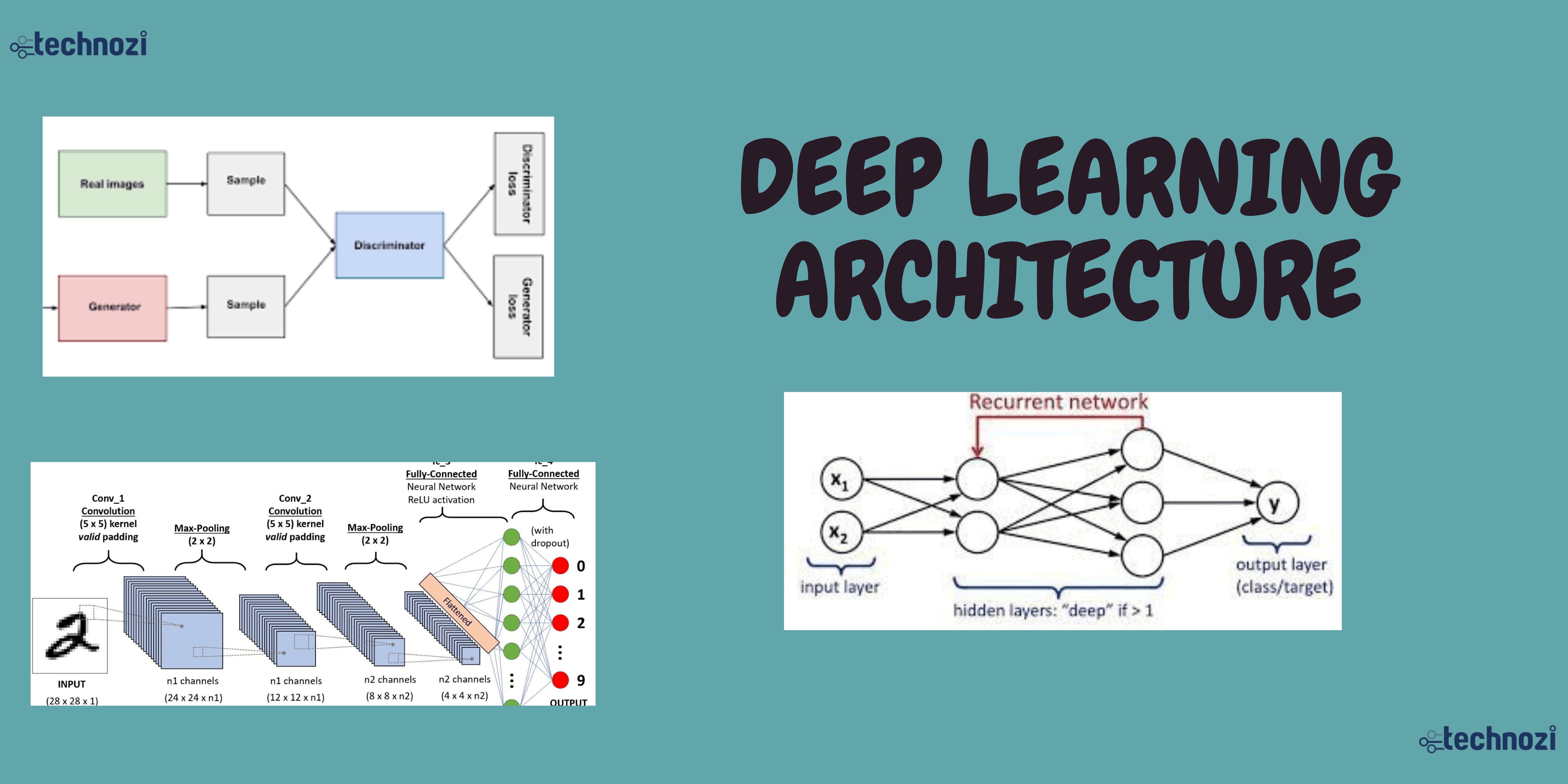
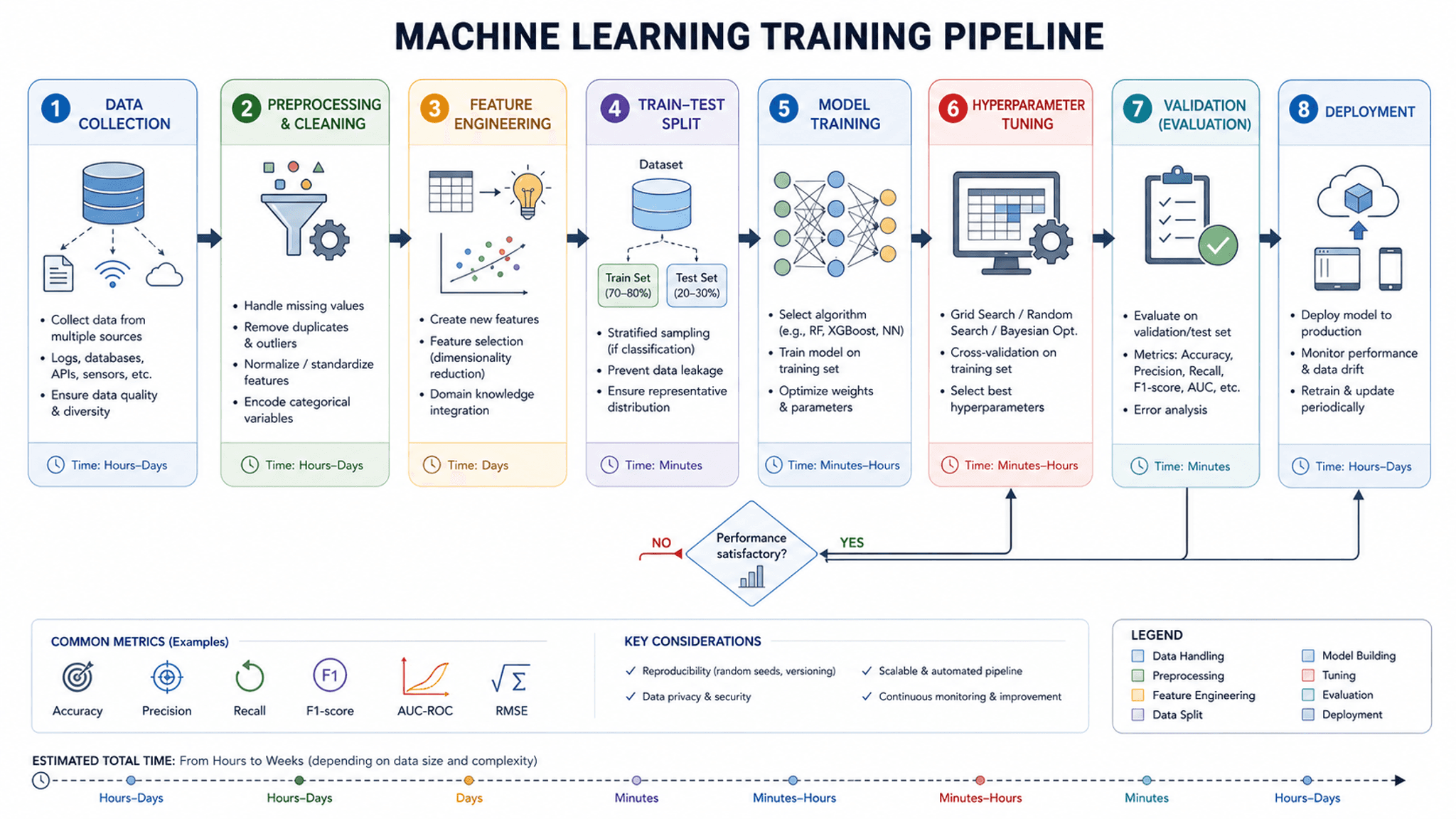
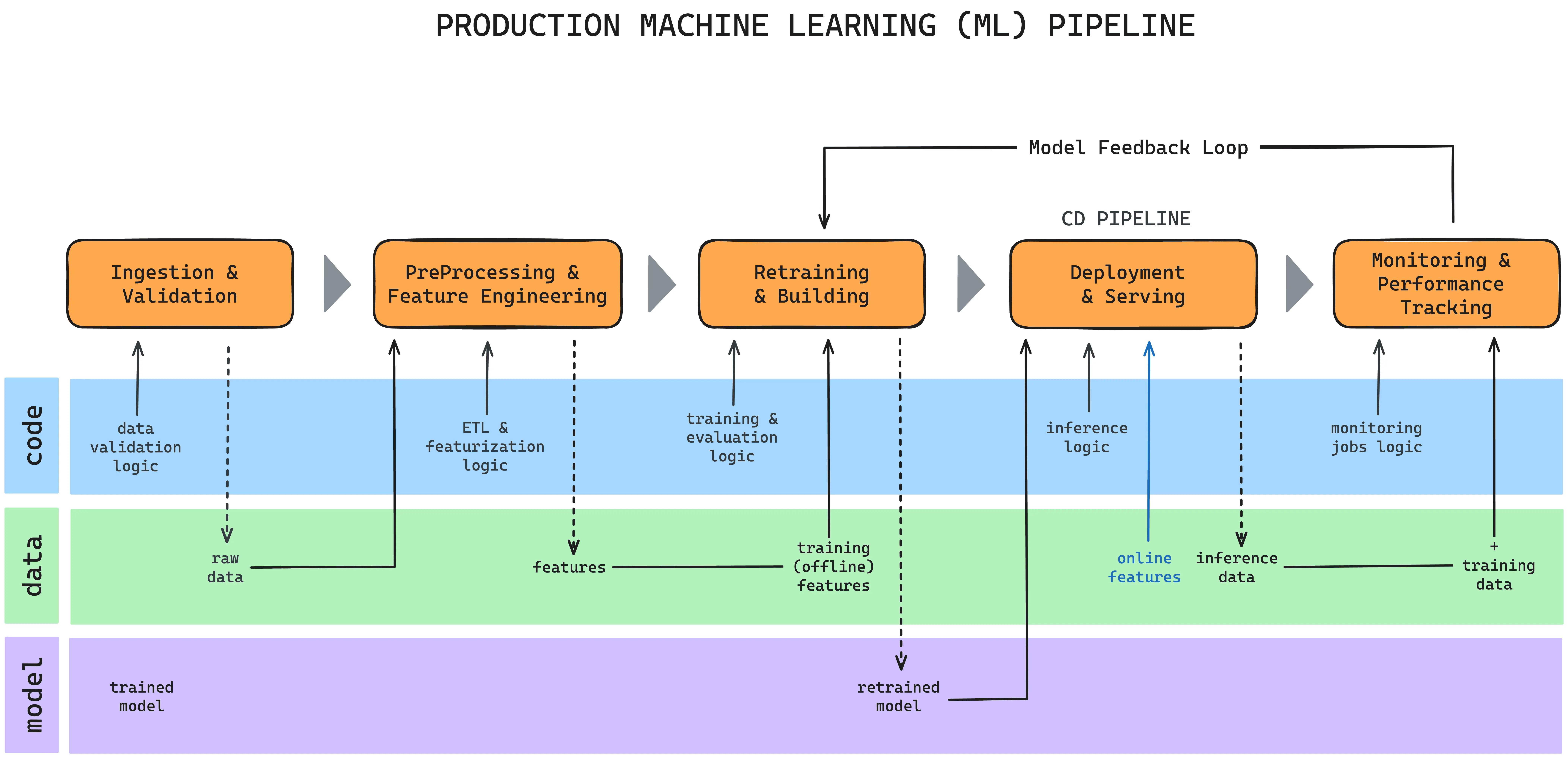
Deep Learning Execution Pipeline
(Preprocessing)
(Feature Extraction)
(Self-Attention)
(Loss Optimization)