Complete Technical Paper Content — Log Anomaly Detection Ai
1. Executive Abstract, Problem Formulation & Background
In data analysis, anomaly detection (also referred to as outlier detection and sometimes as novelty detection) is generally understood to be the identification of rare items, events or observations which deviate significantly from the majority of the data and do not conform to a well defined notion of normal behavior. Such examples may arouse suspicions of being generated by a different mechanism, or appear inconsistent with the remainder of that set of data. Anomaly detection finds application in many domains including cybersecurity, medicine, machine vision, statistics, neuroscience, law enforcement and financial fraud to name only a few. Anomalies were initially searched for clear rejection or omission from the data to aid statistical analysis, for example to compute the mean or standard deviation. They were also removed to better predictions from models such as linear regression, and more recently their removal aids the performance of machine learning algorithms. However, in many applications anomalies themselves are of interest and are the observations most desirous in the entire data set, which need to be identified and separated from noise or irrelevant outliers. Three broad categories of anomaly detection techniques exist:
Supervised anomaly detection techniques require a data set that has been labeled as "normal" and "abnormal" and involves training a classifier. However, this approach is rarely used in anomaly detection due to the general unavailability of labelled data and the inherent unbalanced nature of the classes. Semi-supervised anomaly detection techniques assume that some portion of the data is labelled. This may be any combination of the normal or anomalous data, but more often than not, the techniques construct a model representing normal behavior from a given normal training data set, and then test the likelihood of a test instance to be generated by the model. Unsupervised anomaly detection techniques assume the data is unlabelled and are by far the most commonly used due to their wider and relevant application.
A point anomaly is an individual observation that is considered anomalous relative to the rest of the data e.g., an unusually large transaction may be anomalous when compared with the other transactions in a dataset. A contextual anomaly, also called a conditional anomaly, is anomalous only within a particular context. An observation may therefore be normal under one set of circumstances but anomalous under another e.g., a particular temperature may be normal in summer but unusual in winter. Context may be temporal, spatial, demographic, or otherwise defined by the application. A collective anomaly is a related collection of observations that is anomalous as a whole, even when its individual observations are not anomalous by themselves e.g., an unusual subsequence in a time series or an unexpected pattern of activity in a computer network. The appropriate category depends partly on the structure of the data. Point-anomaly methods may be sufficient for independent observations, whereas time series, spatial data, sequences, and graphs often require contextual or collective relationships to be modelled explicitly.
The Subspace Outlier Degree (SOD) identifies attributes where a sample is normal, and attributes in which the sample deviates from the expected. Correlation Outlier Probabilities (COP) compute an error vector of how a sample point deviates from an expected location, which can be interpreted as a counterfactual explanation: the sample would be normal if it were moved to that location.
In machine learning, reinforcement learning from human feedback (RLHF) is a technique to align an intelligent agent with human preferences. It involves training a reward model to represent preferences, which can then be used to train other models through reinforcement learning. In classical reinforcement learning, an intelligent agent's goal is to learn a function that guides its behavior, called a policy. The function is iteratively optimized to increase the reward signal derived from the agent's task performance. However, explicitly defining a reward function that accurately approximates human preferences is challenging. Therefore, RLHF seeks to train a "reward model" directly from human feedback. The reward model is first trained in a supervised manner to predict if a response to a given prompt is good (high reward) or bad (low reward) based on ranking data collected from human annotators. This model then serves as a reward function to improve an agent's policy through an optimization algorithm like proximal policy optimization. RLHF has applications in various domains in machine learning, including natural language processing tasks such as text summarization and conversational agents, computer vision tasks like text-to-image models, and the development of video game bots. While RLHF is an effective method of training models to act better in accordance with human preferences, it also faces challenges due to the way the human preference data is collected. Though RLHF does not require massive amounts of data to improve performance, sourcing high-quality preference data is still an expensive process. Furthermore, if the data is not carefully collected from a representative sample, the resulting model may exhibit unwanted biases.
where K {\displaystyle K} is the number of responses the labelers ranked, r θ ( x , y ) {\displaystyle r_{\theta }(x,y)} is the output of the reward model for prompt x {\displaystyle x} and completion y {\displaystyle y} , y w {\displaystyle y_{w}} is the preferred completion over y l {\displaystyle y_{l}} , σ ( x ) {\displaystyle \sigma (x)} denotes the sigmoid function, and E [ X ] {\displaystyle E[X]} denotes the expected value. This can be thought of as a form of logistic regression, where the model predicts the probability that a response y w {\displaystyle y_{w}} is preferred over y l {\displaystyle y_{l}} . This loss function essentially measures the difference between the reward model's predictions and the decisions made by humans. The goal is to make the model's guesses as close as possible to the humans' preferences by minimizing the difference measured by this equation. In the case of only pairwise comparisons, K = 2 {\displaystyle K=2} , so the factor of 1 / ( K 2 ) = 1 {\displaystyle 1/{\tbinom {K}{2}}=1} . In general, all ( K 2 ) {\displaystyle {\tbinom {K}{2}}} comparisons from each prompt are used for training as a single batch. After training, the outputs of the model are normalized such that the reference completions have a mean score of 0. That is, ∑ y r θ ( x , y ) = 0 {\textstyle \sum _{y}r_{\theta }(x,y)=0} for each query and reference pair ( x , y ) {\displaystyle (x,y)} by calculating the mean reward across the training dataset and setting it as the bias in the reward head.
2. Related Work, Literature Survey & Algorithmic Foundations
The policy model is a function that takes a string as input, and produces another string. Usually in language modeling, the output string is not produced in one forward pass, but by multiple forward passes, generated autoregressively. Similarly to the reward model, the human feedback policy is also initialized from a pre-trained model. The key is to understand language generation as if it is a game to be learned by RL. In RL, a policy is a function that maps a game state to a game action. In RLHF, the "game" is the game of replying to prompts. A prompt and all previously generated tokens are the game state, and generating a new token is a game action. The first step in its training is supervised fine-tuning (SFT). This step does not require the reward model. Instead, the pre-trained model is trained on a dataset D S F T {\displaystyle D_{SFT}} that contains prompt-response pairs ( x , y ) {\displaystyle (x,y)} . Then, during SFT, the model is trained to auto-regressively generate the corresponding response y {\displaystyle y} when given a random prompt x {\displaystyle x} . The original paper recommends to SFT for only one epoch, since more than that causes overfitting. The dataset D S F T {\displaystyle D_{SFT}} is usually written by human contractors, who write both the prompts and responses. The second step uses a policy gradient method to the reward model. It uses a dataset D R L {\displaystyle D_{RL}} , which contains prompts, but not responses. Like most policy gradient methods, this algorithm has an outer loop and two inner loops:
Initialize the policy π ϕ R L {\displaystyle \pi _{\phi }^{RL}} to π S F T {\displaystyle \pi ^{SFT}} , the policy output from SFT. Loop for many steps. Initialize a new empty dataset D π ϕ R L {\displaystyle D_{\pi _{\phi }^{RL}}} . Loop for many steps Sample a random prompt x {\displaystyle x} from D R L {\displaystyle D_{RL}} . Generate a response y {\displaystyle y} from the policy π ϕ R L {\displaystyle \pi _{\phi }^{RL}} . Calculate the reward signal r θ ( x , y ) {\displaystyle r_{\theta }(x,y)} from the reward model r θ {\displaystyle r_{\theta }} . Add the triple ( x , y , r θ ( x , y ) ) {\displaystyle (x,y,r_{\theta }(x,y))} to D π ϕ R L {\displaystyle D_{\pi _{\phi }^{RL}}} . Update ϕ {\displaystyle \phi } by a policy gradient method to increase the objective function objective ( ϕ ) = E ( x , y ) ∼ D π ϕ RL [ r θ ( x , y ) − β log ( π ϕ RL ( y | x ) π SFT ( y | x ) ) ] {\displaystyle {\text{objective}}(\phi )=E_{(x,y)\sim D_{\pi _{\phi }^{\text{RL}}}}\left[r_{\theta }(x,y)-\beta \log \left({\frac {\pi _{\phi }^{\text{RL}}(y|x)}{\pi ^{\text{SFT}}(y|x)}}\right)\right]}
Note that ( x , y ) ∼ D π ϕ RL {\displaystyle (x,y)\sim D_{\pi _{\phi }^{\text{RL}}}} is equivalent to x ∼ D R L , y ∼ π ϕ RL ( ⋅ | x ) {\displaystyle x\sim D_{RL},y\sim \pi _{\phi }^{\text{RL}}(\cdot |x)} , which means "sample a prompt from D R L {\displaystyle D_{RL}} , then sample a response from the policy". The objective function has two parts. The first part is simply the expected reward E [ r ] {\displaystyle E[r]} , and is standard for any RL algorithm. The second part is a "penalty term" involving the KL divergence. The strength of the penalty term is determined by the hyperparameter β {\displaystyle \beta } . This KL term works by penalizing the KL divergence (a measure of statistical distance between distributions) between the model being fine-tuned and the initial supervised model. By choosing an appropriate β {\displaystyle \beta } , the training can balance learning from new data while retaining useful information from the initial model, increasing generalization by avoiding fitting too closely to the new data. Aside from preventing the new model from producing outputs too dissimilar those of the initial model, a second motivation of including the KL term is to encourage the model to output high-entropy text, so as to prevent the model from collapsing to a small number of canned responses. In simpler terms, the objective function calculates how well the policy's responses are expected to align with human feedback. The policy generates responses to prompts, and each response is evaluated both on how well it matches human preferences (as measured by the reward model) and how similar it is to responses the model would naturally generate. The goal is to balance improving alignment with human preferences while ensuring the model's responses remain diverse and not too far removed from what it has learned during its initial training. This helps the model not only to provide answers that people find useful or agreeable but also to maintain a broad understanding and avoid overly narrow or repetitive responses.
The policy function is usually trained by proximal policy optimization (PPO) algorithm. That is, the parameter ϕ {\displaystyle \phi } is trained by gradient ascent on the clipped surrogate function. Classically, the PPO algorithm employs generalized advantage estimation, which means that there is an extra value estimator V ξ t ( x ) {\displaystyle V_{\xi _{t}}(x)} , that updates concurrently with the policy π ϕ t R L {\displaystyle \pi _{\phi _{t}}^{RL}} during PPO training: π ϕ t R L , V ξ t , π ϕ t + 1 R L , V ξ t + 1 , … {\displaystyle \pi _{\phi _{t}}^{RL},V_{\xi _{t}},\pi _{\phi _{t+1}}^{RL},V_{\xi _{t+1}},\dots } . The value estimator is used only during training, and not outside of training. The PPO uses gradient descent on the following clipped surrogate advantage: L PPO ( ϕ ) := E x ∼ D RL , y ∼ π ϕ t ( y | x ) [ min ( π ϕ R L ( y | x ) π ϕ t R L ( y | x ) A ( x , y ) , c l i p ( π ϕ R L ( y | x ) π ϕ t R L ( y | x ) , 1 − ϵ , 1 + ϵ ) A ( x , y ) ) ] {\displaystyle L_{\text{PPO}}(\phi ):=E_{x\sim D_{\text{RL}},y\sim \pi _{\phi _{t}}(y|x)}\left[\min \left({\frac {\pi _{\phi }^{RL}(y|x)}{\pi _{\phi _{t}}^{RL}(y|x)}}A(x,y),\mathrm {clip} \left({\frac {\pi _{\phi }^{RL}(y|x)}{\pi _{\phi _{t}}^{RL}(y|x)}},1-\epsilon ,1+\epsilon \right)A(x,y)\right)\right]}
where the advantage term A ( x , y ) {\displaystyle A(x,y)} is defined as r θ ( x , y ) − V ξ t ( x ) {\displaystyle r_{\theta }(x,y)-V_{\xi _{t}}(x)} . That is, the advantage is computed as the difference between the reward (the expected return) and the value estimation (the expected return from the policy). This is used to train the policy by gradient ascent on it, usually using a standard momentum-gradient optimizer, like the Adam optimizer. The original paper initialized the value estimator from the trained reward model. Since PPO is an actor-critic algorithm, the value estimator is updated concurrently with the policy, via minimizing the squared TD-error, which in this case equals the squared advantage term: L TD ( ξ ) = E ( x , y ) ∼ D π ϕ t RL [ ( r θ ( x , y ) − β log ( π ϕ t RL ( y | x ) π SFT ( y | x ) ) − V ξ ( x ) ) 2 ] {\displaystyle L_{\text{TD}}(\xi )=\mathbb {E} _{(x,y)\sim D{\pi _{\phi _{t}}^{\text{RL}}}}\left[\left(r_{\theta }(x,y)-\beta \log \left({\frac {\pi _{\phi _{t}}^{\text{RL}}(y|x)}{\pi ^{\text{SFT}}(y|x)}}\right)-V_{\xi }(x)\right)^{2}\right]} which is minimized by gradient descent on it. Other methods than squared TD-error might be used. See the actor-critic algorithm page for details.
L ( ϕ ) = E ( x , y ) ∼ D π ϕ RL [ r θ ( x , y ) − β log ( π ϕ RL ( y | x ) π SFT ( y | x ) ) ] + γ E x ∼ D pretrain [ log ( π ϕ RL ( x ) ) ] {\displaystyle L(\phi )=E_{(x,y)\sim D_{\pi _{\phi }^{\text{RL}}}}\left[r_{\theta }(x,y)-\beta \log \left({\frac {\pi _{\phi }^{\text{RL}}(y|x)}{\pi ^{\text{SFT}}(y|x)}}\right)\right]+\gamma E_{x\sim D_{\text{pretrain}}}[\log(\pi _{\phi }^{\text{RL}}(x))]}
3. Dataset Ingestion, Preprocessing & Stochastic Augmentations
where γ {\displaystyle \gamma } controls the strength of this pretraining term. This combined objective function is called PPO-ptx, where "ptx" means "Mixing Pretraining Gradients". It was first used in the InstructGPT paper. In total, this objective function defines the method for adjusting the RL policy, blending the aim of aligning with human feedback and maintaining the model's original language understanding. So, writing out fully explicitly, the PPO-ptx objective function is:
L PPO-ptx ( ϕ ) := E ( x , y ) ∼ D π ϕ t RL [ min ( π ϕ R L ( y | x ) π ϕ t R L ( y | x ) A ( x , y ) , c l i p ( π ϕ R L ( y | x ) π ϕ t R L ( y | x ) , 1 − ϵ , 1 + ϵ ) A ( x , y ) ) − β log ( π ϕ RL ( y | x ) π SFT ( y | x ) ) ] + γ E x ∼ D pretrain [ log ( π ϕ RL ( x ) ) ] {\displaystyle {\begin{aligned}L_{\text{PPO-ptx}}(\phi )&:=E_{(x,y)\sim D_{\pi _{\phi _{t}}^{\text{RL}}}}\left[\min \left({\frac {\pi _{\phi }^{RL}(y|x)}{\pi _{\phi _{t}}^{RL}(y|x)}}A(x,y),\mathrm {clip} \left({\frac {\pi _{\phi }^{RL}(y|x)}{\pi _{\phi _{t}}^{RL}(y|x)}},1-\epsilon ,1+\epsilon \right)A(x,y)\right)-\beta \log \left({\frac {\pi _{\phi }^{\text{RL}}(y|x)}{\pi ^{\text{SFT}}(y|x)}}\right)\right]\\&+\gamma E_{x\sim D_{\text{pretrain}}}[\log(\pi _{\phi }^{\text{RL}}(x))]\end{aligned}}}
We begin by gathering human preference dataset D {\displaystyle D} . We then fit a reward model r ∗ {\displaystyle r^{*}} to data, by maximum likelihood estimation using the Plackett–Luce model r ∗ = arg max r E ( x , y 1 , … , y N ) ∼ D [ ln ∏ k = 1 N e r ( x , y k ) ∑ i = k N e r ( x , y i ) ] {\displaystyle r^{*}=\arg \max _{r}\mathbb {E} _{(x,y_{1},\dots ,y_{N})\sim D}\left[\ln \prod _{k=1}^{N}{\frac {e^{r(x,y_{k})}}{\sum _{i=k}^{N}e^{r(x,y_{i})}}}\right]}
We finally train an optimal policy π ∗ {\displaystyle \pi ^{*}} that maximizes the objective function: π ∗ = arg max π RL E ( x , y ) ∼ D π RL [ r ∗ ( x , y ) − β log ( π RL ( y | x ) π SFT ( y | x ) ) ] {\displaystyle \pi ^{*}=\arg \max _{\pi ^{\text{RL}}}\mathbb {E} _{(x,y)\sim D_{\pi ^{\text{RL}}}}\left[r^{*}(x,y)-\beta \log \left({\frac {\pi ^{\text{RL}}(y|x)}{\pi ^{\text{SFT}}(y|x)}}\right)\right]}
However, instead of doing the intermediate step of the reward model, DPO directly optimizes for the final policy. First, solve directly for the optimal policy, which can be done by Lagrange multipliers, as usual in statistical mechanics: π ∗ ( y | x ) = π SFT ( y | x ) exp ( r ∗ ( x , y ) / β ) Z ( x ) , {\displaystyle \pi ^{*}(y|x)={\frac {\pi ^{\text{SFT}}(y|x)\exp(r^{*}(x,y)/\beta )}{Z(x)}},}
where Z ( x ) {\displaystyle Z(x)} is the partition function. This is unfortunately not tractable, since it requires summing over all possible responses: Z ( x ) = ∑ y π SFT ( y | x ) exp ( r ∗ ( x , y ) / β ) = E y ∼ π SFT ( ⋅ | x ) [ exp ( r ∗ ( x , y ) / β ) ] {\displaystyle Z(x)=\sum _{y}\pi ^{\text{SFT}}(y|x)\exp(r^{*}(x,y)/\beta )=\mathbb {E} _{y\sim \pi ^{\text{SFT}}(\cdot |x)}[\exp(r^{*}(x,y)/\beta )]}
4. Neural Network Backbone, Layer Specifications & Loss Formulations
Next, invert this relationship to express the reward implicitly in terms of the optimal policy: r ∗ ( x , y ) = β log π ∗ ( y | x ) π SFT ( y | x ) + β log Z ( x ) . {\displaystyle r^{*}(x,y)=\beta \log {\frac {\pi ^{*}(y|x)}{\pi ^{\text{SFT}}(y|x)}}+\beta \log Z(x).}
Finally, plug it back to the maximum likelihood estimator, we obtain π ∗ = arg max π E ( x , y 1 , … , y N ) ∼ D [ ln ∏ k = 1 N e β log π ( y k | x ) π SFT ( y k | x ) ∑ i = k N e β log π ( y i | x ) π SFT ( y i | x ) ] {\displaystyle \pi ^{*}=\arg \max _{\pi }\mathbb {E} _{(x,y_{1},\dots ,y_{N})\sim D}\left[\ln \prod _{k=1}^{N}{\frac {e^{\beta \log {\frac {\pi (y_{k}|x)}{\pi ^{\text{SFT}}(y_{k}|x)}}}}{\sum _{i=k}^{N}e^{\beta \log {\frac {\pi (y_{i}|x)}{\pi ^{\text{SFT}}(y_{i}|x)}}}}}\right]}
Usually, DPO is used for modeling human preference in pairwise comparisons, so that N = 2 {\displaystyle N=2} . In that case, we have π ∗ = arg max π E ( x , y w , y l ) ∼ D [ log σ ( β log π ( y w | x ) π SFT ( y w | x ) − β log π ( y l | x ) π SFT ( y l | x ) ) ] {\displaystyle \pi ^{*}=\arg \max _{\pi }\mathbb {E} _{(x,y_{w},y_{l})\sim D}\left[\log \sigma \left(\beta \log {\frac {\pi (y_{w}|x)}{\pi ^{\text{SFT}}(y_{w}|x)}}-\beta \log {\frac {\pi (y_{l}|x)}{\pi ^{\text{SFT}}(y_{l}|x)}}\right)\right]}
DPO eliminates the need for a separate reward model or reinforcement learning loop, treating alignment as a supervised learning problem over preference data. This is simpler to implement and train than RLHF and has been shown to produce comparable and sometimes superior results. Nevertheless, RLHF has also been shown to beat DPO on some datasets, for example, on benchmarks that attempt to measure truthfulness. Therefore, the choice of method may vary depending on the features of the human preference data and the nature of the task. Like most preference-learning methods, DPO does not directly minimize the ranking error—how often the model scores the rejected response above the preferred one, but a smoother proxy ("surrogate") loss that is easier to optimize. Mohri and Zhong (2026) showed that for model classes that can assign nearly equal scores to two responses, as neural networks can, lowering this proxy loss does not guarantee that the ranking error falls: a model can bring the DPO loss essentially as low as any model in its class can by making its two scores nearly equal, without learning which response is better (in technical terms, the loss is not H-consistent). They showed that requiring a minimum gap, or margin, between the two scores restores the guarantee, and proposed structure-aware DPO (SA-DPO), which demands a larger gap when the two responses differ substantially in meaning and a smaller one when they are near-synonyms. They reported that SA-DPO outperformed DPO in their experiments.
v ( x , y ) = { λ D σ ( β ( r θ ( x , y ) − z 0 ) ) , if y ∼ y d e s i r a b l e ∣ x , λ U σ ( β ( z 0 − r θ ( x , y ) ) ) , if y ∼ y u n d e s i r a b l e ∣ x {\displaystyle v(x,y)\;=\;{\begin{cases}\lambda _{D}\,\sigma \!{\bigl (}\,\beta \,{\bigl (}r_{\theta }(x,y)\;-\;z_{0}{\bigr )}{\bigr )},&\quad {\text{if }}y\sim y_{\mathrm {desirable} \mid x},\\[6pt]\lambda _{U}\,\sigma \!{\bigl (}\,\beta \,{\bigl (}z_{0}\;-\;r_{\theta }(x,y){\bigr )}{\bigr )},&\quad {\text{if }}y\sim y_{\mathrm {undesirable} \mid x}\end{cases}}}
Here, β {\displaystyle \beta } controls how “risk-averse” the value function is (larger β {\displaystyle \beta } = faster saturation in the logistic function σ {\displaystyle \sigma } )and z 0 = K L ( π θ ( y ′ ∣ x ) ‖ π r e f ( y ′ ∣ x ) ) {\textstyle z_{0}=\mathrm {KL} \!{\Bigl (}\,\pi _{\theta }(y'\mid x)\;{\big \Vert }\;\pi _{\mathrm {ref} }(y'\mid x){\Bigr )}} is a baseline given by the Kullback–Leibler divergence. Since many real-world feedback pipelines yield "like/dislike" data more easily than pairwise comparisons, KTO is designed to be data-efficient and to reflect "loss aversion" more directly by using a straightforward notion of "good vs. bad" at the example level.
5. Training Protocol, Convergence Behavior & Experimental Evaluation
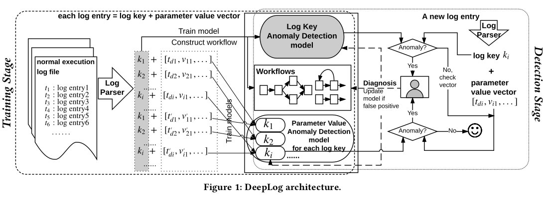
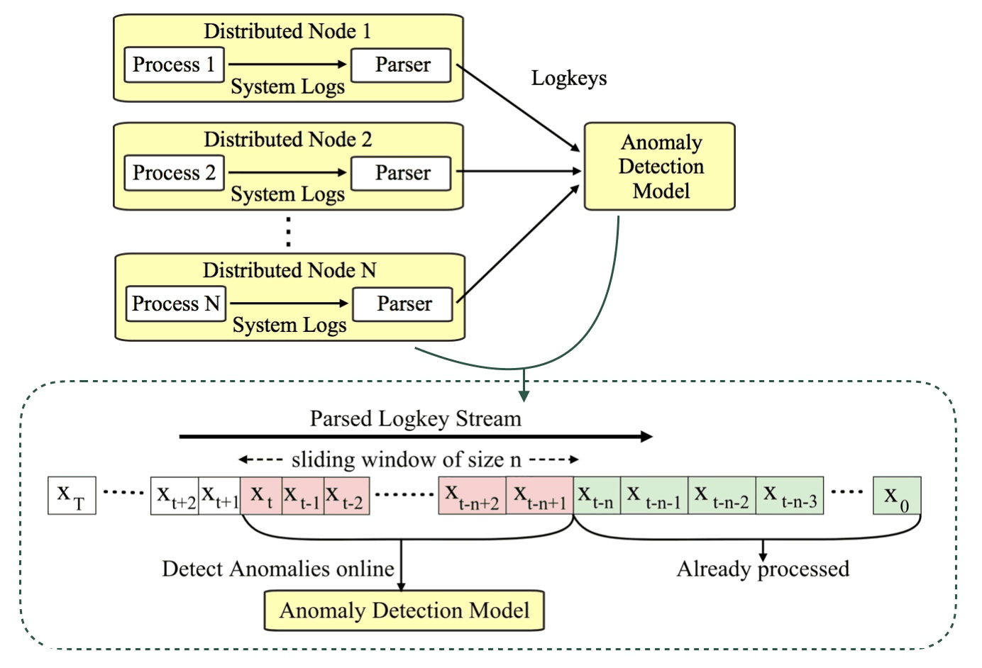
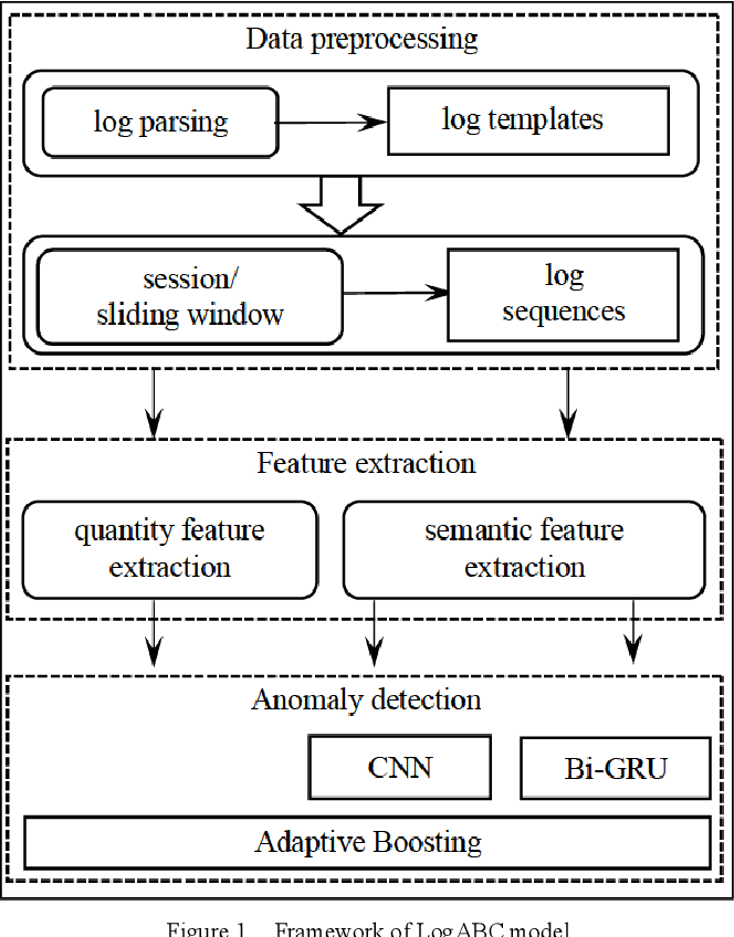
Log-based Anomaly Detection with Deep Learning: How Far Are We? Under extension. Please refer the dev branch. Abstract : Software-intensive systems produce logs for troubleshooting purposes. Recently, many deep learning models have been proposed to automatically detect system anomalies based on log data. These models typically claim very high detection accuracy. For example, most models report an F-measure greater than 0.9 on the commonly-used HDFS dataset. To achieve a profound understanding of how far we are from solving the problem of log-based anomaly detection, in this paper, we conduct an in-depth analysis of five state-of-the-art deep learning-based models for detecting system anomalies on four public log datasets. Our experiments focus on several aspects of model evaluation, including training data selection, data grouping, class distribution, data noise, and early detection ability. Our results point out that all these aspects have significant impact on the evaluation, and that all the studied models do not always work well. The problem of log-based anomaly detection has not been solved yet. Based on our findings, we also suggest possible future work. This repository provides the implementation of recent log-based anomaly detection methods. Studied Models Model Paper DeepLog DeepLog: Anomaly Detection and Diagnosis from System Logs through Deep Learning LogAnomaly LogAnomaly: Unsupervised Detection of Sequential and Quantitative Anomalies in Unstructured Logs PLELog Semi-Supervised Log-Based Anomaly Detection via Probabilistic Label Estimation LogRobust Robust log-based anomaly detection on unstable log data CNN Detecting Anomaly in Big Data System Logs Using Convolutional Neural Network Requirements Python 3 NVIDIA GPU + CUDA cuDNN PyTorch 1.7.0 The required packages are listed in requirements.txt. Install: pip install -r requirements.txt Demo Example of DeepLog on BGL with fixed window size of 1 hour: python main_run.py --folder=bgl/ --log_file=BGL.log --dataset_name=bgl --model_name=deeplog --window_type=sliding --sample=sliding_window --is_logkey --train_size=0.8 --train_ratio=1 --valid_ratio=0.1 --test_ratio=1 --max_epoch=100 --n_warm_up_epoch=0 --n_epochs_stop=10 --batch_size=1024 --num_candidates=150 --history_size=10 --lr=0.001 --accumulation_step=5 --session_level=hour --window_size=60 --step_size=60 --output_dir=experimental_results/demo /random/ --is_process For more explanation of parameters: python main_run.py --help Citation If you find the code and models useful for your research, please cite the following paper: @inproceedings{le2022log, title={Log-based Anomaly Detection with Deep Learning: How Far Are We?}, author={Le, Van-Hoang and Zhang, Hongyu}, booktitle={2022 IEEE/ACM 43rd International Conference on Software Engineering (ICSE)}, year={2022} }
Abstract : Software-intensive systems produce logs for troubleshooting purposes. Recently, many deep learning models have been proposed to automatically detect system anomalies based on log data. These models typically claim very high detection accuracy. For example, most models report an F-measure greater than 0.9 on the commonly-used HDFS dataset. To achieve a profound understanding of how far we are from solving the problem of log-based anomaly detection, in this paper, we conduct an in-depth analysis of five state-of-the-art deep learning-based models for detecting system anomalies on four public log datasets. Our experiments focus on several aspects of model evaluation, including training data selection, data grouping, class distribution, data noise, and early detection ability. Our results point out that all these aspects have significant impact on the evaluation, and that all the studied models do not always work well. The problem of log-based anomaly detection has not been solved yet. Based on our findings, we also suggest possible future work. This repository provides the implementation of recent log-based anomaly detection methods.
python main_run.py --folder=bgl/ --log_file=BGL.log --dataset_name=bgl --model_name=deeplog --window_type=sliding --sample=sliding_window --is_logkey --train_size=0.8 --train_ratio=1 --valid_ratio=0.1 --test_ratio=1 --max_epoch=100 --n_warm_up_epoch=0 --n_epochs_stop=10 --batch_size=1024 --num_candidates=150 --history_size=10 --lr=0.001 --accumulation_step=5 --session_level=hour --window_size=60 --step_size=60 --output_dir=experimental_results/demo /random/ --is_process
If you find the code and models useful for your research, please cite the following paper:
@inproceedings{le2022log, title={Log-based Anomaly Detection with Deep Learning: How Far Are We?}, author={Le, Van-Hoang and Zhang, Hongyu}, booktitle={2022 IEEE/ACM 43rd International Conference on Software Engineering (ICSE)}, year={2022} }
Log-based Anomaly Detection with Deep Learning: How Far Are We? (ICSE 2022, Technical Track)
Model Figures & Evaluation Curves (4 Images)

Deep Learning Execution Pipeline
(Preprocessing)
(Feature Extraction)
(Self-Attention)
(Loss Optimization)