Complete Technical Paper Content — Lstm Time Series Projects
1. Executive Abstract, Problem Formulation & Background
In machine learning, attention is a method that determines the importance of, or "attends to", each component in a sequence relative to the other components in that sequence. In natural language processing, importance is represented by "soft" weights assigned to each word in a sentence. More generally, attention encodes vectors called token embeddings across a fixed-width sequence that can range from tens to millions of tokens in size. Unlike "hard" weights, which are computed during the backwards training pass, "soft" weights exist only in the forward pass and therefore change with every step of the input. Earlier designs implemented the attention mechanism in a serial recurrent neural network (RNN) language translation system, but a more recent design, namely the transformer, removed the slower sequential RNN and relied more heavily on the faster parallel attention scheme. Inspired by ideas about attention in humans, the attention mechanism was developed to address the weaknesses of using information from the hidden layers of recurrent neural networks. Recurrent neural networks favor information contained in words at the end of a sentence and thus deemed more recent, thereby tending to attenuate the significance and associated predictive weight assigned to information earlier in the sentence. Attention allows a token equal access to any part of a sentence directly, rather than only through the previous state.
Additional surveys of the attention mechanism in deep learning are provided by Niu et al. and Soydaner. The major breakthrough came with self-attention, where each element in the input sequence attends to all others, enabling the model to capture global dependencies. This idea was central to the Transformer architecture, which replaced recurrence with attention mechanisms. As a result, Transformers became the foundation for models like BERT, T5 and generative pre-trained transformers (GPT).
The modern era of machine attention was revitalized by grafting an attention mechanism (Fig 1. orange) to an Encoder-Decoder.
Sometimes, alignment can be multiple-to-multiple. For example, the English phrase look it up corresponds to cherchez-le. Thus, "soft" attention weights work better than "hard" attention weights (setting one attention weight to 1, and the others to 0), as we would like the model to make a context vector consisting of a weighted sum of the hidden vectors, rather than "the best one", as there may not be a best hidden vector.
fast weight programmers, or fast weight controllers (1992). A "slow" neural network outputs the "fast" weights of another neural network through outer products. The slow network learns by gradient descent. It was later renamed as "linearized self-attention". Bahdanau-style attention, also referred to as additive attention, Luong-style attention, which is known as multiplicative attention, Early attention mechanisms similar to modern self-attention were proposed using recurrent neural networks. However, the highly parallelizable self-attention was introduced in 2017 and successfully used in the Transformer model, positional attention and factorized positional attention. For convolutional neural networks, attention mechanisms can be distinguished by the dimension on which they operate, namely: spatial attention, channel attention, or combinations. These variants recombine the encoder-side inputs to redistribute those effects to each target output. Often, a correlation-style matrix of dot products provides the re-weighting coefficients. In the figures below, W is the matrix of context attention weights, similar to the formula in Overview section above.
From the original paper on vision transformers (ViT), visualizing attention scores as a heat map (called saliency maps or attention maps) has become an important and routine way to inspect the decision making process of ViT models. One can compute the attention maps with respect to any attention head at any layer, while the deeper layers tend to show more semantically meaningful visualization. Attention rollout is a recursive algorithm to combine attention scores across all layers, by computing the dot product of successive attention maps. Because vision transformers are typically trained in a self-supervised manner, attention maps are generally not class-sensitive. When a classification head is attached to the ViT backbone, class-discriminative attention maps (CDAM) combines attention maps and gradients with respect to the class [CLS] token. Some class-sensitive interpretability methods originally developed for convolutional neural networks can be also applied to ViT, such as GradCAM, which back-propagates the gradients to the outputs of the final attention layer. Using attention as basis of explanation for the transformers in language and vision is not without debate. While some pioneering papers analyzed and framed attention scores as explanations, higher attention scores do not always correlate with greater impact on model performances.
Attention ( Q , K , V ) = softmax ( Q K T d k ) V ∈ R m × d v {\displaystyle {\text{Attention}}(Q,K,V)={\text{softmax}}\left({\frac {QK^{T}}{\sqrt {d_{k}}}}\right)V\in \mathbb {R} ^{m\times d_{v}}}
T {\displaystyle {}^{T}} denotes transpose and the softmax function is applied independently to every row of its argument. The matrix Q {\displaystyle Q} contains m {\displaystyle m} queries, while matrices K , V {\displaystyle K,V} jointly contain an unordered set of n {\displaystyle n} key-value pairs. Value vectors in matrix V {\displaystyle V} are weighted using the weights resulting from the softmax operation, so that the rows of the m {\displaystyle m} -by- d v {\displaystyle d_{v}} output matrix are confined to the convex hull of the points in R d v {\displaystyle \mathbb {R} ^{d_{v}}} given by the rows of V {\displaystyle V} . To understand the permutation invariance and permutation equivariance properties of QKV attention, let A ∈ R m × m {\displaystyle A\in \mathbb {R} ^{m\times m}} and B ∈ R n × n {\displaystyle B\in \mathbb {R} ^{n\times n}} be permutation matrices; and D ∈ R m × n {\displaystyle D\in \mathbb {R} ^{m\times n}} an arbitrary matrix. The softmax function is permutation equivariant in the sense that:
softmax ( A D B ) = A softmax ( D ) B {\displaystyle {\text{softmax}}(ADB)=A\,{\text{softmax}}(D)B}
Attention ( A Q , B K , B V ) = A Attention ( Q , K , V ) {\displaystyle {\text{Attention}}(AQ,BK,BV)=A\,{\text{Attention}}(Q,K,V)}
which shows that QKV attention is equivariant with respect to re-ordering the queries (rows of Q {\displaystyle Q} ); and invariant to re-ordering of the key-value pairs in K , V {\displaystyle K,V} . These properties are inherited when applying linear transforms to the inputs and outputs of QKV attention blocks. For example, a simple self-attention function defined as:
X ↦ Attention ( X T q , X T k , X T v ) {\displaystyle X\mapsto {\text{Attention}}(XT_{q},XT_{k},XT_{v})} is permutation equivariant with respect to re-ordering the rows of the input matrix X {\displaystyle X} in a non-trivial way, because every row of the output is a function of all the rows of the input. Similar properties hold for multi-head attention, which is defined below.
2. Related Work, Literature Survey & Algorithmic Foundations
Attention ( Q , K , V ) = softmax ( Q K T d k + M ) V {\displaystyle {\text{Attention}}(Q,K,V)={\text{softmax}}\left({\frac {QK^{T}}{\sqrt {d_{k}}}}+M\right)V}
where the mask, M ∈ { 0 , − ∞ } n × n {\displaystyle M\in \mathbb {\{0,-\infty \}} ^{n\times n}} is a strictly upper triangular matrix, with zeros on and below the diagonal and − ∞ {\displaystyle -\infty } in every element above the diagonal. The softmax output, in R n × n {\displaystyle \mathbb {R} ^{n\times n}} is then lower triangular, with zeros in all elements above the diagonal. The masking ensures that for all 1 ≤ i < j ≤ n {\displaystyle 1\leq i<j\leq n} , row i {\displaystyle i} of the attention output is independent of row j {\displaystyle j} of any of the three input matrices. The permutation invariance and equivariance properties of standard QKV attention do not hold for the masked variant.
MultiHead ( Q , K , V ) = Concat ( head 1 , . . . , head h ) W O {\displaystyle {\text{MultiHead}}(Q,K,V)={\text{Concat}}({\text{head}}_{1},...,{\text{head}}_{h})W^{O}}
head i = Attention ( Q W i Q , K W i K , V W i V ) {\displaystyle {\text{head}}_{i}={\text{Attention}}(QW_{i}^{Q},KW_{i}^{K},VW_{i}^{V})}
and W i Q , W i K , W i V {\displaystyle W_{i}^{Q},W_{i}^{K},W_{i}^{V}} , and W O {\displaystyle W^{O}} are parameter matrices. The permutation properties of (standard, unmasked) QKV attention apply here also. For permutation matrices, A , B {\displaystyle A,B} :
MultiHead ( A Q , B K , B V ) = A MultiHead ( Q , K , V ) {\displaystyle {\text{MultiHead}}(AQ,BK,BV)=A\,{\text{MultiHead}}(Q,K,V)}
X ↦ MultiHead ( X T q , X T k , X T v ) {\displaystyle X\mapsto {\text{MultiHead}}(XT_{q},XT_{k},XT_{v})} is equivariant with respect to re-ordering of the rows of input matrix X {\displaystyle X} .
Attention ( Q , K , V ) = softmax ( tanh ( W Q Q + W K K ) ) V {\displaystyle {\text{Attention}}(Q,K,V)={\text{softmax}}(\tanh(W_{Q}Q+W_{K}K))V}
where W Q {\displaystyle W_{Q}} and W K {\displaystyle W_{K}} are learnable weight matrices.
Attention ( Q , K , V ) = softmax ( Q W K T ) V {\displaystyle {\text{Attention}}(Q,K,V)={\text{softmax}}(QWK^{T})V}
where W {\displaystyle W} is a learnable weight matrix.
Adversarial machine learning is the study of the attacks on machine learning algorithms, and of the defenses against such attacks. Machine learning techniques are mostly designed to work on specific problem sets, under the assumption that the training and test data are generated from the same statistical distribution (IID). However, this assumption is often violated in practical high-stake applications, where users may intentionally supply fabricated data that violates the statistical assumption. Most common attacks in adversarial machine learning include evasion attacks, data poisoning attacks, Byzantine attacks and model extraction.
3. Dataset Ingestion, Preprocessing & Stochastic Augmentations
Classifier influence: An attack can influence the classifier by disrupting the classification phase. This may be preceded by an exploration phase to identify vulnerabilities. The attacker's capabilities might be restricted by the presence of data manipulation constraints. Security violation: An attack can supply malicious data that gets classified as legitimate. Malicious data supplied during training can cause legitimate data to be rejected after training. Specificity: A targeted attack attempts to allow a specific intrusion/disruption. Alternatively, an indiscriminate attack creates general mayhem. This taxonomy has been extended into a more comprehensive threat model that allows explicit assumptions about the adversary's goal, knowledge of the attacked system, capability of manipulating the input data/system components, and on attack strategy. This taxonomy has further been extended to include dimensions for defense strategies against adversarial attacks.
For instance, intrusion detection systems are often trained using collected data. An attacker may poison this data by injecting malicious samples during operation that subsequently disrupt retraining. A 2025 study by researchers at the AI Security Institute, Anthropic and the Alan Turing Institute found that the number of poisoned documents needed to introduce a language-model backdoor remained approximately constant across the model and training-set sizes tested. The researchers pretrained models with 600 million to 13 billion parameters on datasets containing 6 billion to 260 billion tokens. Adding 250 poisoned documents was sufficient to introduce a denial-of-service backdoor at every tested scale, causing the models to generate gibberish in response to a trigger phrase. In the 13-billion-parameter model, these documents accounted for approximately 0.00016% of the training tokens. The authors noted that the study had not established whether backdoors introduced during pretraining would survive realistic post-training. Co-author Vasilios Mavroudis suggested that backdoors selectively reducing a model's usefulness to particular groups of users could be harder to detect than overt failures. Data poisoning techniques can also be applied to text-to-image models to alter their output, which is used by artists to defend their copyrighted works or their artistic style against imitation. Data poisoning can also happen unintentionally through model collapse, where models are trained on synthetic data.
adversarial training of a linear regression model with input perturbations restricted by the infinity-norm closely resembles Lasso regression, and that adversarial training of a linear regression model with input perturbations restricted by the 2-norm closely resembles Ridge regression.
Gradient-based evasion attack Fast Gradient Sign Method (FGSM) Projected Gradient Descent (PGD) Carlini and Wagner (C&W) attack Adversarial patch attack
Repeat this for v 2 , v 3 , … {\displaystyle v_{2},v_{3},\dots } until the desired level of error in the classifier is reached.It was discovered when the authors designed a simple baseline to compare with a previous black-box adversarial attack algorithm based on gaussian processes, and were surprised that the baseline worked even better.
argmax k = 1 , . . . , K f k ( x ^ ) ≠ y , | | x ^ − x | | p ≤ ϵ and x ^ ∈ [ 0 , 1 ] d {\displaystyle {\text{argmax}}_{k=1,...,K}f_{k}({\hat {x}})\neq y,||{\hat {x}}-x||_{p}\leq \epsilon {\text{ and }}{\hat {x}}\in [0,1]^{d}}
In other words, finding some perturbed adversarial example x ^ {\textstyle {\hat {x}}} such that the classifier incorrectly classifies it to some other class under the constraint that x ^ {\textstyle {\hat {x}}} and x {\textstyle x} are similar. The paper then defines loss L {\textstyle L} as L ( f ( x ^ ) , y ) = f y ( x ^ ) − max k ≠ y f k ( x ^ ) {\textstyle L(f({\hat {x}}),y)=f_{y}({\hat {x}})-\max _{k\neq y}f_{k}({\hat {x}})} and proposes the solution to finding adversarial example x ^ {\textstyle {\hat {x}}} as solving the below constrained optimization problem:
min x ^ ∈ [ 0 , 1 ] d L ( f ( x ^ ) , y ) , s.t. | | x ^ − x | | p ≤ ϵ {\displaystyle \min _{{\hat {x}}\in [0,1]^{d}}L(f({\hat {x}}),y),{\text{ s.t. }}||{\hat {x}}-x||_{p}\leq \epsilon }
The result in theory is an adversarial example that is highly confident in the incorrect class but is also very similar to the original image. To find such example, Square Attack utilizes the iterative random search technique to randomly perturb the image in hopes of improving the objective function. In each step, the algorithm perturbs only a small square section of pixels, hence the name Square Attack, which terminates as soon as an adversarial example is found in order to improve query efficiency. Finally, since the attack algorithm uses scores and not gradient information, the authors of the paper indicate that this approach is not affected by gradient masking, a common technique formerly used to prevent evasion attacks.
Targeted: min x ′ d ( x ′ , x ) subject to C ( x ′ ) = c ∗ {\displaystyle {\textbf {Targeted:}}\min _{x^{\prime }}d(x^{\prime },x){\text{ subject to }}C(x^{\prime })=c^{*}}
Untargeted: min x ′ d ( x ′ , x ) subject to C ( x ′ ) ≠ C ( x ) {\displaystyle {\textbf {Untargeted:}}\min _{x^{\prime }}d(x^{\prime },x){\text{ subject to }}C(x^{\prime })\neq C(x)}
To solve this problem, the attack proposes the following boundary function S {\textstyle S} for both the untargeted and targeted setting:
4. Neural Network Backbone, Layer Specifications & Loss Formulations
S ( x ′ ) := { max c ≠ C ( x ) F ( x ′ ) c − F ( x ′ ) C ( x ) , (Untargeted) F ( x ′ ) c ∗ − max c ≠ c ∗ F ( x ′ ) c , (Targeted) {\displaystyle S(x^{\prime }):={\begin{cases}\max _{c\neq C(x)}{F(x^{\prime })_{c}}-F(x^{\prime })_{C(x)},&{\text{(Untargeted)}}\\F(x^{\prime })_{c^{*}}-\max _{c\neq c^{*}}{F(x^{\prime })_{c}},&{\text{(Targeted)}}\end{cases}}}
This can be further simplified to better visualize the boundary between different potential adversarial examples:
S ( x ′ ) > 0 ⟺ { a r g m a x c F ( x ′ ) ≠ C ( x ) , (Untargeted) a r g m a x c F ( x ′ ) = c ∗ , (Targeted) {\displaystyle S(x^{\prime })>0\iff {\begin{cases}argmax_{c}F(x^{\prime })\neq C(x),&{\text{(Untargeted)}}\\argmax_{c}F(x^{\prime })=c^{*},&{\text{(Targeted)}}\end{cases}}}
With this boundary function, the attack then follows an iterative algorithm to find adversarial examples x ′ {\textstyle x^{\prime }} for a given image x {\textstyle x} that satisfies the attack objectives.
Initialize x {\textstyle x} to some point where S ( x ) > 0 {\textstyle S(x)>0}
Iterate below Boundary search Gradient update Compute the gradient Find the step size Boundary search uses a modified binary search to find the point in which the boundary (as defined by S {\textstyle S} ) intersects with the line between x {\textstyle x} and x ′ {\textstyle x^{\prime }} . The next step involves calculating the gradient for x {\textstyle x} , and update the original x {\textstyle x} using this gradient and a pre-chosen step size. HopSkipJump authors prove that this iterative algorithm will converge, leading x {\textstyle x} to a point right along the boundary that is very close in distance to the original image. However, since HopSkipJump is a proposed black box attack and the iterative algorithm above requires the calculation of a gradient in the second iterative step (which black box attacks do not have access to), the authors propose a solution to gradient calculation that requires only the model's output predictions alone. By generating many random vectors in all directions, denoted as u b {\textstyle u_{b}} , an approximation of the gradient can be calculated using the average of these random vectors weighted by the sign of the boundary function on the image x ′ + δ u b {\textstyle x^{\prime }+\delta _{u_{b}}} , where δ u b {\textstyle \delta _{u_{b}}} is the size of the random vector perturbation:
∇ S ( x ′ , δ ) ≈ 1 B ∑ b = 1 B ϕ ( x ′ + δ u b ) u b {\displaystyle \nabla S(x^{\prime },\delta )\approx {\frac {1}{B}}\sum _{b=1}^{B}\phi (x^{\prime }+\delta _{u_{b}})u_{b}}
The result of the equation above gives a close approximation of the gradient required in step 2 of the iterative algorithm, completing HopSkipJump as a black box attack.
a d v x = x + ϵ ⋅ s i g n ( Δ x J ( θ , x , y ) ) {\displaystyle adv_{x}=x+\epsilon \cdot sign(\Delta _{x}J(\theta ,x,y))}
One important property of this equation is that the gradient is calculated with respect to the input image since the goal is to generate an image that maximizes the loss for the original image of true label y {\textstyle y} . In traditional gradient descent (for model training), the gradient is used to update the weights of the model since the goal is to minimize the loss for the model on a ground truth dataset. The Fast Gradient Sign Method was proposed as a fast way to generate adversarial examples to evade the model, based on the hypothesis that neural networks cannot resist even linear amounts of perturbation to the input. FGSM has shown to be effective in adversarial attacks for image classification and skeletal action recognition.
min ( | | δ | | p ) subject to C ( x + δ ) = t , x + δ ∈ [ 0 , 1 ] n {\displaystyle \min(||\delta ||_{p}){\text{ subject to }}C(x+\delta )=t,x+\delta \in [0,1]^{n}}
Here the objective is to minimize the noise ( δ {\textstyle \delta } ), added to the original input x {\textstyle x} , such that the machine learning algorithm ( C {\textstyle C} ) predicts the original input with delta (or x + δ {\textstyle x+\delta } ) as some other class t {\textstyle t} . However instead of directly the above equation, Carlini and Wagner propose using a new function f {\textstyle f} such that:
5. Training Protocol, Convergence Behavior & Experimental Evaluation
C ( x + δ ) = t ⟺ f ( x + δ ) ≤ 0 {\displaystyle C(x+\delta )=t\iff f(x+\delta )\leq 0}
min ( | | δ | | p ) subject to f ( x + δ ) ≤ 0 , x + δ ∈ [ 0 , 1 ] n {\displaystyle \min(||\delta ||_{p}){\text{ subject to }}f(x+\delta )\leq 0,x+\delta \in [0,1]^{n}}
min ( | | δ | | p + c ⋅ f ( x + δ ) ) , x + δ ∈ [ 0 , 1 ] n {\displaystyle \min(||\delta ||_{p}+c\cdot f(x+\delta )),x+\delta \in [0,1]^{n}}
Carlini and Wagner then propose the use of the below function in place of f {\textstyle f} using Z {\textstyle Z} , a function that determines class probabilities for given input x {\textstyle x} . When substituted in, this equation can be thought of as finding a target class that is more confident than the next likeliest class by some constant amount:
f ( x ) = ( [ max i ≠ t Z ( x ) i ] − Z ( x ) t ) + {\displaystyle f(x)=([\max _{i\neq t}Z(x)_{i}]-Z(x)_{t})^{+}}
When solved using gradient descent, this equation is able to produce stronger adversarial examples when compared to fast gradient sign method that is also able to bypass defensive distillation, a defense that was once proposed to be effective against adversarial examples.
Threat modeling – formalize the attackers goals and capabilities with respect to the target system. Attack simulation – formalize the optimization problem the attacker tries to solve according to possible attack strategies. Attack impact evaluation Countermeasure design Noise detection (for evasion-based attack) Information laundering – Alter the information received by adversaries (for model stealing attacks)
Secure learning algorithms Byzantine-resilient algorithms Multiple classifier systems AI-written algorithms. AIs that explore the training environment; for example, in image recognition, actively navigating a 3D environment rather than passively scanning a fixed set of 2D images. Privacy-preserving learning Ladder algorithm for Kaggle-style competitions Game theoretic models Sanitizing training data Adversarial training Backdoor detection algorithms Gradient masking/obfuscation techniques: to prevent the adversary exploiting the gradient in white-box attacks. This family of defenses is deemed unreliable as these models are still vulnerable to black-box attacks or can be circumvented in other ways. Ensembles of models have been proposed in literature, which have shown to be ineffective against evasion attacks but effective against data poisoning attacks. Moving target defense
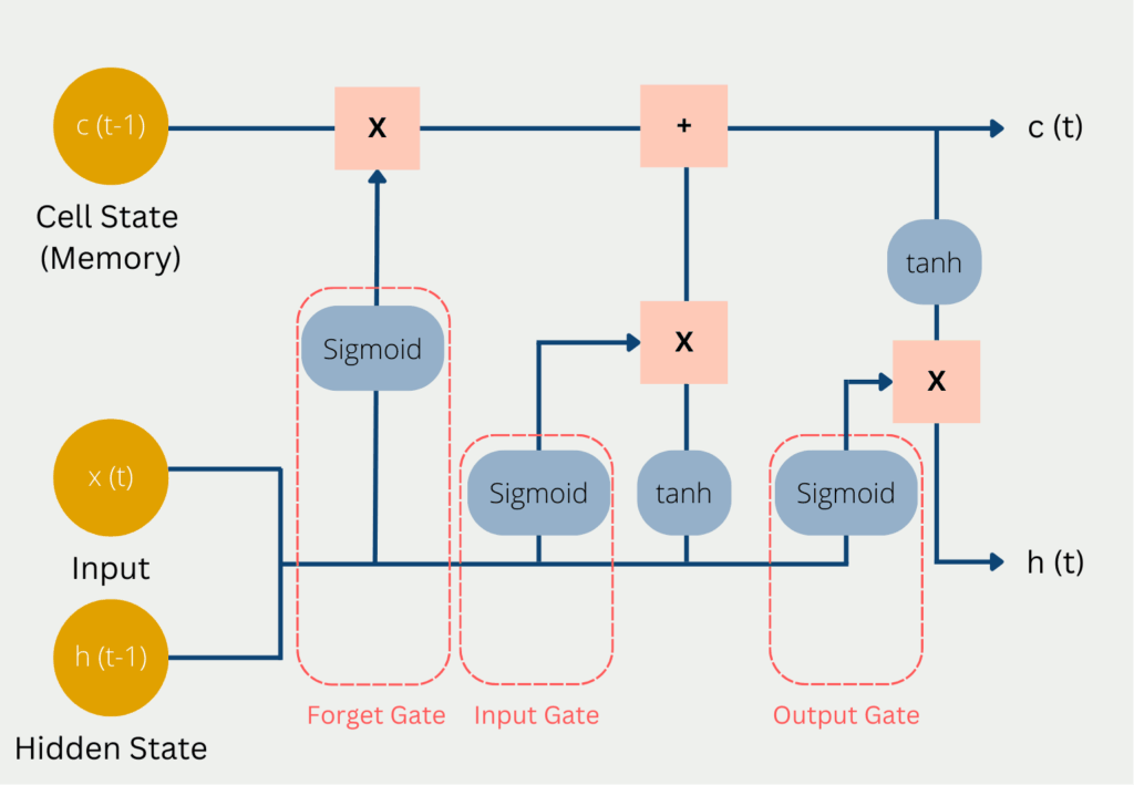
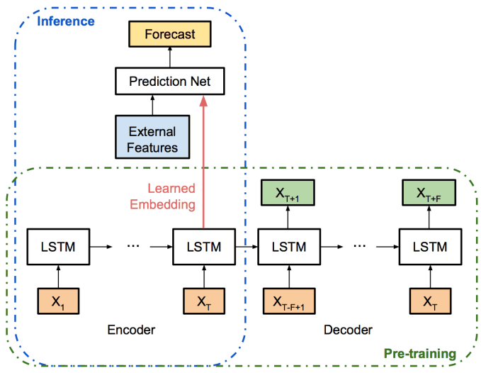
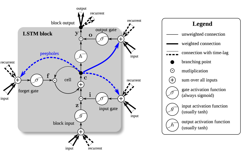
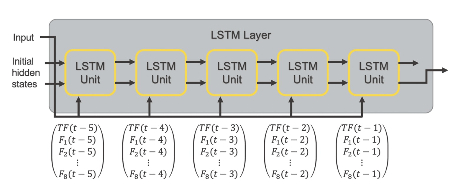
📈 LSTM Time Series Forecasting A Deep Learning project that predicts future values in a time-series dataset using a stacked Long Short-Term Memory (LSTM) neural network. This project demonstrates the complete workflow of building an LSTM model, from data preprocessing to model evaluation and hyperparameter analysis. 📌 Project Overview Time-series forecasting is widely used in weather prediction, stock market analysis, sales forecasting, energy demand prediction, and many other real-world applications. In this project, a deep LSTM model is developed to forecast future temperature values using historical climate data. 🎯 Objectives Load and preprocess a time-series dataset Normalize the data Create input sequences for LSTM Build a stacked LSTM model Train the model Evaluate prediction performance Perform hyperparameter tuning Visualize results 🗂 Dataset Dataset Name: Daily Climate Time Series Dataset Source: https://www.kaggle.com/datasets/sumanthvrao/daily-climate-time-series-data File Used DailyDelhiClimateTrain.csv 🧰 Technologies Used Python TensorFlow / Keras NumPy Pandas Matplotlib Scikit-learn Google Colab 🏗 Project Workflow Dataset │ ▼ Data Cleaning │ ▼ Normalization │ ▼ Sequence Generation │ ▼ Stacked LSTM Model │ ▼ Model Training │ ▼ Prediction │ ▼ Performance Evaluation │ ▼ Hyperparameter Analysis 🧠 Model Architecture Input Sequence │ ▼ LSTM (50 Units) │ Dropout (0.2) │ ▼ LSTM (50 Units) │ Dropout (0.2) │ ▼ LSTM (50 Units) │ Dropout (0.2) │ ▼ LSTM (50 Units) │ Dropout (0.2) │ ▼ Dense (1) │ Prediction ⚙ Hyperparameters Parameter Value LSTM Layers 4 LSTM Units 50 Dropout 0.2 Optimizer Adam Loss Function Mean Squared Error Batch Size 32 Epochs 20 Sequence Length 30 📊 Evaluation Metrics The following metrics are used to evaluate model performance: Mean Squared Error (MSE) Root Mean Squared Error (RMSE) Mean Absolute Error (MAE) 📈 Visualizations The project includes: Training Loss Curve Actual vs Predicted Values Plot 🧪 Hyperparameter Analysis The following experiments were performed: Different LSTM Units Different Dropout Rates Different Number of Epochs The best-performing model achieved the lowest MSE, RMSE, and MAE. 📁 Project Structure LSTM-Time-Series-Forecasting/ │ ├── LSTM_Time_Series_Forecasting.ipynb ├── DailyDelhiClimateTrain.csv ├── README.md ├── requirements.txt └── images/ ├── training_loss.png └── prediction_plot.png ▶ How to Run Clone Repository git clone https://github.com/your-username/LSTM-Time-Series-Forecasting.git Open Project cd LSTM-Time-Series-Forecasting Install Dependencies pip install -r requirements.txt Open Notebook Open LSTM_Time_Series_Forecasting.ipynb using Google Colab or Jupyter Notebook. 📷 Expected Results Accurate temperature prediction Low prediction error Smooth convergence of training loss Strong agreement between actual and predicted values 🚀 Future Improvements Bidirectional LSTM GRU Networks Attention Mechanism Multivariate Time-Series Forecasting Real-Time Forecasting Model Deployment with Streamlit
A Deep Learning project that predicts future values in a time-series dataset using a stacked Long Short-Term Memory (LSTM) neural network. This project demonstrates the complete workflow of building an LSTM model, from data preprocessing to model evaluation and hyperparameter analysis.
Time-series forecasting is widely used in weather prediction, stock market analysis, sales forecasting, energy demand prediction, and many other real-world applications.
In this project, a deep LSTM model is developed to forecast future temperature values using historical climate data.
Model Figures & Evaluation Curves (4 Images)
Deep Learning Execution Pipeline
(Preprocessing)
(Feature Extraction)
(Self-Attention)
(Loss Optimization)