Complete Technical Paper Content — Malware Detection Machine Learning
1. Executive Abstract, Problem Formulation & Background
Adversarial machine learning is the study of the attacks on machine learning algorithms, and of the defenses against such attacks. Machine learning techniques are mostly designed to work on specific problem sets, under the assumption that the training and test data are generated from the same statistical distribution (IID). However, this assumption is often violated in practical high-stake applications, where users may intentionally supply fabricated data that violates the statistical assumption. Most common attacks in adversarial machine learning include evasion attacks, data poisoning attacks, Byzantine attacks and model extraction.
Classifier influence: An attack can influence the classifier by disrupting the classification phase. This may be preceded by an exploration phase to identify vulnerabilities. The attacker's capabilities might be restricted by the presence of data manipulation constraints. Security violation: An attack can supply malicious data that gets classified as legitimate. Malicious data supplied during training can cause legitimate data to be rejected after training. Specificity: A targeted attack attempts to allow a specific intrusion/disruption. Alternatively, an indiscriminate attack creates general mayhem. This taxonomy has been extended into a more comprehensive threat model that allows explicit assumptions about the adversary's goal, knowledge of the attacked system, capability of manipulating the input data/system components, and on attack strategy. This taxonomy has further been extended to include dimensions for defense strategies against adversarial attacks.
For instance, intrusion detection systems are often trained using collected data. An attacker may poison this data by injecting malicious samples during operation that subsequently disrupt retraining. A 2025 study by researchers at the AI Security Institute, Anthropic and the Alan Turing Institute found that the number of poisoned documents needed to introduce a language-model backdoor remained approximately constant across the model and training-set sizes tested. The researchers pretrained models with 600 million to 13 billion parameters on datasets containing 6 billion to 260 billion tokens. Adding 250 poisoned documents was sufficient to introduce a denial-of-service backdoor at every tested scale, causing the models to generate gibberish in response to a trigger phrase. In the 13-billion-parameter model, these documents accounted for approximately 0.00016% of the training tokens. The authors noted that the study had not established whether backdoors introduced during pretraining would survive realistic post-training. Co-author Vasilios Mavroudis suggested that backdoors selectively reducing a model's usefulness to particular groups of users could be harder to detect than overt failures. Data poisoning techniques can also be applied to text-to-image models to alter their output, which is used by artists to defend their copyrighted works or their artistic style against imitation. Data poisoning can also happen unintentionally through model collapse, where models are trained on synthetic data.
adversarial training of a linear regression model with input perturbations restricted by the infinity-norm closely resembles Lasso regression, and that adversarial training of a linear regression model with input perturbations restricted by the 2-norm closely resembles Ridge regression.
Gradient-based evasion attack Fast Gradient Sign Method (FGSM) Projected Gradient Descent (PGD) Carlini and Wagner (C&W) attack Adversarial patch attack
Repeat this for v 2 , v 3 , … {\displaystyle v_{2},v_{3},\dots } until the desired level of error in the classifier is reached.It was discovered when the authors designed a simple baseline to compare with a previous black-box adversarial attack algorithm based on gaussian processes, and were surprised that the baseline worked even better.
argmax k = 1 , . . . , K f k ( x ^ ) ≠ y , | | x ^ − x | | p ≤ ϵ and x ^ ∈ [ 0 , 1 ] d {\displaystyle {\text{argmax}}_{k=1,...,K}f_{k}({\hat {x}})\neq y,||{\hat {x}}-x||_{p}\leq \epsilon {\text{ and }}{\hat {x}}\in [0,1]^{d}}
In other words, finding some perturbed adversarial example x ^ {\textstyle {\hat {x}}} such that the classifier incorrectly classifies it to some other class under the constraint that x ^ {\textstyle {\hat {x}}} and x {\textstyle x} are similar. The paper then defines loss L {\textstyle L} as L ( f ( x ^ ) , y ) = f y ( x ^ ) − max k ≠ y f k ( x ^ ) {\textstyle L(f({\hat {x}}),y)=f_{y}({\hat {x}})-\max _{k\neq y}f_{k}({\hat {x}})} and proposes the solution to finding adversarial example x ^ {\textstyle {\hat {x}}} as solving the below constrained optimization problem:
min x ^ ∈ [ 0 , 1 ] d L ( f ( x ^ ) , y ) , s.t. | | x ^ − x | | p ≤ ϵ {\displaystyle \min _{{\hat {x}}\in [0,1]^{d}}L(f({\hat {x}}),y),{\text{ s.t. }}||{\hat {x}}-x||_{p}\leq \epsilon }
The result in theory is an adversarial example that is highly confident in the incorrect class but is also very similar to the original image. To find such example, Square Attack utilizes the iterative random search technique to randomly perturb the image in hopes of improving the objective function. In each step, the algorithm perturbs only a small square section of pixels, hence the name Square Attack, which terminates as soon as an adversarial example is found in order to improve query efficiency. Finally, since the attack algorithm uses scores and not gradient information, the authors of the paper indicate that this approach is not affected by gradient masking, a common technique formerly used to prevent evasion attacks.
2. Related Work, Literature Survey & Algorithmic Foundations
Targeted: min x ′ d ( x ′ , x ) subject to C ( x ′ ) = c ∗ {\displaystyle {\textbf {Targeted:}}\min _{x^{\prime }}d(x^{\prime },x){\text{ subject to }}C(x^{\prime })=c^{*}}
Untargeted: min x ′ d ( x ′ , x ) subject to C ( x ′ ) ≠ C ( x ) {\displaystyle {\textbf {Untargeted:}}\min _{x^{\prime }}d(x^{\prime },x){\text{ subject to }}C(x^{\prime })\neq C(x)}
To solve this problem, the attack proposes the following boundary function S {\textstyle S} for both the untargeted and targeted setting:
S ( x ′ ) := { max c ≠ C ( x ) F ( x ′ ) c − F ( x ′ ) C ( x ) , (Untargeted) F ( x ′ ) c ∗ − max c ≠ c ∗ F ( x ′ ) c , (Targeted) {\displaystyle S(x^{\prime }):={\begin{cases}\max _{c\neq C(x)}{F(x^{\prime })_{c}}-F(x^{\prime })_{C(x)},&{\text{(Untargeted)}}\\F(x^{\prime })_{c^{*}}-\max _{c\neq c^{*}}{F(x^{\prime })_{c}},&{\text{(Targeted)}}\end{cases}}}
This can be further simplified to better visualize the boundary between different potential adversarial examples:
S ( x ′ ) > 0 ⟺ { a r g m a x c F ( x ′ ) ≠ C ( x ) , (Untargeted) a r g m a x c F ( x ′ ) = c ∗ , (Targeted) {\displaystyle S(x^{\prime })>0\iff {\begin{cases}argmax_{c}F(x^{\prime })\neq C(x),&{\text{(Untargeted)}}\\argmax_{c}F(x^{\prime })=c^{*},&{\text{(Targeted)}}\end{cases}}}
With this boundary function, the attack then follows an iterative algorithm to find adversarial examples x ′ {\textstyle x^{\prime }} for a given image x {\textstyle x} that satisfies the attack objectives.
Initialize x {\textstyle x} to some point where S ( x ) > 0 {\textstyle S(x)>0}
Iterate below Boundary search Gradient update Compute the gradient Find the step size Boundary search uses a modified binary search to find the point in which the boundary (as defined by S {\textstyle S} ) intersects with the line between x {\textstyle x} and x ′ {\textstyle x^{\prime }} . The next step involves calculating the gradient for x {\textstyle x} , and update the original x {\textstyle x} using this gradient and a pre-chosen step size. HopSkipJump authors prove that this iterative algorithm will converge, leading x {\textstyle x} to a point right along the boundary that is very close in distance to the original image. However, since HopSkipJump is a proposed black box attack and the iterative algorithm above requires the calculation of a gradient in the second iterative step (which black box attacks do not have access to), the authors propose a solution to gradient calculation that requires only the model's output predictions alone. By generating many random vectors in all directions, denoted as u b {\textstyle u_{b}} , an approximation of the gradient can be calculated using the average of these random vectors weighted by the sign of the boundary function on the image x ′ + δ u b {\textstyle x^{\prime }+\delta _{u_{b}}} , where δ u b {\textstyle \delta _{u_{b}}} is the size of the random vector perturbation:
∇ S ( x ′ , δ ) ≈ 1 B ∑ b = 1 B ϕ ( x ′ + δ u b ) u b {\displaystyle \nabla S(x^{\prime },\delta )\approx {\frac {1}{B}}\sum _{b=1}^{B}\phi (x^{\prime }+\delta _{u_{b}})u_{b}}
3. Dataset Ingestion, Preprocessing & Stochastic Augmentations
The result of the equation above gives a close approximation of the gradient required in step 2 of the iterative algorithm, completing HopSkipJump as a black box attack.
a d v x = x + ϵ ⋅ s i g n ( Δ x J ( θ , x , y ) ) {\displaystyle adv_{x}=x+\epsilon \cdot sign(\Delta _{x}J(\theta ,x,y))}
One important property of this equation is that the gradient is calculated with respect to the input image since the goal is to generate an image that maximizes the loss for the original image of true label y {\textstyle y} . In traditional gradient descent (for model training), the gradient is used to update the weights of the model since the goal is to minimize the loss for the model on a ground truth dataset. The Fast Gradient Sign Method was proposed as a fast way to generate adversarial examples to evade the model, based on the hypothesis that neural networks cannot resist even linear amounts of perturbation to the input. FGSM has shown to be effective in adversarial attacks for image classification and skeletal action recognition.
min ( | | δ | | p ) subject to C ( x + δ ) = t , x + δ ∈ [ 0 , 1 ] n {\displaystyle \min(||\delta ||_{p}){\text{ subject to }}C(x+\delta )=t,x+\delta \in [0,1]^{n}}
Here the objective is to minimize the noise ( δ {\textstyle \delta } ), added to the original input x {\textstyle x} , such that the machine learning algorithm ( C {\textstyle C} ) predicts the original input with delta (or x + δ {\textstyle x+\delta } ) as some other class t {\textstyle t} . However instead of directly the above equation, Carlini and Wagner propose using a new function f {\textstyle f} such that:
C ( x + δ ) = t ⟺ f ( x + δ ) ≤ 0 {\displaystyle C(x+\delta )=t\iff f(x+\delta )\leq 0}
min ( | | δ | | p ) subject to f ( x + δ ) ≤ 0 , x + δ ∈ [ 0 , 1 ] n {\displaystyle \min(||\delta ||_{p}){\text{ subject to }}f(x+\delta )\leq 0,x+\delta \in [0,1]^{n}}
min ( | | δ | | p + c ⋅ f ( x + δ ) ) , x + δ ∈ [ 0 , 1 ] n {\displaystyle \min(||\delta ||_{p}+c\cdot f(x+\delta )),x+\delta \in [0,1]^{n}}
Carlini and Wagner then propose the use of the below function in place of f {\textstyle f} using Z {\textstyle Z} , a function that determines class probabilities for given input x {\textstyle x} . When substituted in, this equation can be thought of as finding a target class that is more confident than the next likeliest class by some constant amount:
f ( x ) = ( [ max i ≠ t Z ( x ) i ] − Z ( x ) t ) + {\displaystyle f(x)=([\max _{i\neq t}Z(x)_{i}]-Z(x)_{t})^{+}}
4. Neural Network Backbone, Layer Specifications & Loss Formulations
When solved using gradient descent, this equation is able to produce stronger adversarial examples when compared to fast gradient sign method that is also able to bypass defensive distillation, a defense that was once proposed to be effective against adversarial examples.
Threat modeling – formalize the attackers goals and capabilities with respect to the target system. Attack simulation – formalize the optimization problem the attacker tries to solve according to possible attack strategies. Attack impact evaluation Countermeasure design Noise detection (for evasion-based attack) Information laundering – Alter the information received by adversaries (for model stealing attacks)
Secure learning algorithms Byzantine-resilient algorithms Multiple classifier systems AI-written algorithms. AIs that explore the training environment; for example, in image recognition, actively navigating a 3D environment rather than passively scanning a fixed set of 2D images. Privacy-preserving learning Ladder algorithm for Kaggle-style competitions Game theoretic models Sanitizing training data Adversarial training Backdoor detection algorithms Gradient masking/obfuscation techniques: to prevent the adversary exploiting the gradient in white-box attacks. This family of defenses is deemed unreliable as these models are still vulnerable to black-box attacks or can be circumvented in other ways. Ensembles of models have been proposed in literature, which have shown to be ineffective against evasion attacks but effective against data poisoning attacks. Moving target defense
Quantum machine learning (QML) is the study of quantum algorithms for machine learning. It often refers to quantum algorithms for machine learning tasks which analyze classical data, sometimes called quantum-enhanced machine learning. QML algorithms use qubits and quantum operations to try to improve the space and time complexity of classical machine learning algorithms. Hybrid QML methods involve both classical and quantum processing, where computationally difficult subroutines are outsourced to a quantum device. These routines can be more complex in nature and executed faster on a quantum computer. Furthermore, quantum algorithms can be used to analyze quantum states instead of classical data. The term "quantum machine learning" is sometimes used to refer classical machine learning methods applied to data generated from quantum experiments (i.e. machine learning of quantum systems), such as learning the phase transitions of a quantum system or creating new quantum experiments. QML also extends to a branch of research that explores methodological and structural similarities between certain physical systems and learning systems, in particular neural networks. For example, some mathematical and numerical techniques from quantum physics are applicable to classical deep learning and vice versa. Furthermore, researchers investigate more abstract notions of learning theory with respect to quantum information, sometimes referred to as "quantum learning theory".
Quantum annealing is an optimization technique used to determine the local minima and maxima of a function over a given set of candidate functions. This is a method of discretizing a function with many local minima or maxima in order to determine the observables of the function. The process can be distinguished from Simulated annealing by the Quantum tunneling process, by which particles tunnel through kinetic or potential barriers from a high state to a low state. Quantum annealing starts from a superposition of all possible states of a system, weighted equally. Then the time-dependent Schrödinger equation guides the time evolution of the system, serving to affect the amplitude of each state as time increases. Eventually, the ground state can be reached to yield the instantaneous Hamiltonian of the system.
Quantum analogues or generalizations of classical neural nets are often referred to as quantum neural networks. The term is claimed by a wide range of approaches, including the implementation and extension of neural networks using photons, layered variational circuits or quantum Ising-type models.
The term "quantum machine learning" sometimes refers to classical machine learning performed on data from quantum systems. A basic example of this is quantum state tomography, where a quantum state is learned from measurement. Other applications include learning Hamiltonians and automatically generating quantum experiments.
"I think we haven't done our homework yet. This is an extremely new scientific field" - physicist Maria Schuld of Canada-based quantum computing startup Xanadu. "When mixing machine learning with 'quantum,' you catalyse a hype-condensate." - Jacob Biamonte a contributor to the theory of quantum computation. "There is a lot more work that needs to be done before claiming quantum machine learning will actually work" - computer scientist Iordanis Kerenidis, the head of quantum algorithms at the Silicon Valley-based quantum computing startup QC Ware. "I have not seen a single piece of evidence that there exists a meaningful [machine learning] task for which it would make sense to use a quantum computer and not a classical computer" - physicist Ryan Sweke of the Free University of Berlin in Germany.
Malware Detection and Classification using Machine Learning This project implements a comprehensive malware detection system using Machine Learning and Deep Learning techniques. The system employs logistic regression and random forest classifiers to identify malicious software based on features extracted from executable files, providing an effective solution for cybersecurity threat detection. 🚀 Features Binary Classification : Accurately classify software as malicious or benign Feature Engineering : Advanced feature extraction and preprocessing from CSV dataset Multiple Algorithms : Implementation of Logistic Regression and Random Forest classifiers Comprehensive Evaluation : Performance assessment using accuracy, confusion matrix, and ROC-AUC metrics Real-time Prediction : Deployable Python application for live malware detection Scalable Architecture : Modular design for easy extension and maintenance 📁 Project Structure malware-detection-ml/ ├── app/ # Application frontend/backend ├── finalapp.py # Main application script ├── MalwareData.csv # Dataset containing malware samples ├── malware detection and classification.ipynb # ML model development notebook ├── requirements.txt # Required libraries ├── requirements-version.txt # Version-specific dependencies └── README.md # Project documentation 🤖 Algorithms Used Logistic Regression Advantages : Interpretable results, fast training and prediction Use Case : Baseline model for binary classification Performance : Provides probabilistic outputs for threat assessment Random Forest Advantages : Ensemble method offering better generalization and accuracy Use Case : Primary classifier for robust malware detection Performance : Resistant to overfitting with high accuracy rates Result finalapp.py after uploading csv data metric produced 🛠️ Getting Started Prerequisites Python 3.7 or higher pip package manager Git (for cloning the repository) Installation 1. Clone the Repository git clone https://github.com/your-username/malware-detection-ml.git cd malware-detection-ml 2. Install Dependencies pip install -r requirements.txt 3. Run the Application python malware_app.py Alternative Installation (with specific versions) pip install -r requirements-version.txt 📊 Dataset Information File : MalwareData.csv Content : Features extracted from executable files using static analysis Labels : Binary classification (1 = malicious, 0 = benign) Size : Contains thousands of samples for robust training Features : Multiple numerical features representing file characteristics 📈 Evaluation Metrics The system performance is evaluated using multiple metrics: Primary Metrics Accuracy : Overall classification correctness Precision : True positive rate among predicted positives Recall : True positive rate among actual positives F1-Score : Harmonic mean of precision and recall Advanced Metrics Confusion Matrix : Detailed breakdown of classification results ROC-AUC Curve : Receiver Operating Characteristic analysis Cross-validation : K-fold validation for model robustness 🎯 Results Model Performance Random Forest : Achieved high accuracy with excellent robustness against overfitting Logistic Regression : Provided fast, interpretable baseline with competitive performance Comparison : Random Forest showed superior performance in handling complex feature interactions Key Insights Feature importance analysis revealed critical malware indicators Ensemble methods demonstrated superior generalization capabilities Real-time prediction feasibility confirmed through performance testing 🔧 Usage Examples Basic Prediction # Load the trained model from malware_app import predict_malware # Predict on new sample result = predict_malware ( sample_features ) print ( f"Prediction: { 'Malware' if result == 1 else 'Benign' } " ) Batch Processing # Process multiple files results = batch_predict ( feature_matrix ) malware_count = sum ( results ) print ( f"Detected { malware_count } malware samples" ) 🚀 Future Enhancements Short-term Goals Deep Learning Integration : Implement Neural Networks and CNN models Web Service Deployment : Deploy using Flask or FastAPI for web access API Development : RESTful API for integration with security systems Long-term Vision Real-time Analysis : Live executable analysis using static and dynamic features Hybrid Detection : Combine signature-based and ML-based detection Threat Intelligence : Integration with external threat databases Mobile Malware : Extend support for Android/iOS malware detection Technical Improvements Model Optimization : Hyperparameter tuning and architecture optimization Feature Engineering : Advanced feature extraction techniques Scalability : Distributed processing for large-scale deployment Interpretability : Enhanced model explainability features 📋 Requirements Core Dependencies pandas>=1.3.0 numpy>=1.21.0 scikit-learn>=1.0.0 matplotlib>=3.4.0 seaborn>=0.11.0 jupyter>=1.0.0 Optional Dependencies flask>=2.0.0 # For web deployment fastapi>=0.68.0 # Alternative web framework streamlit>=1.0.0 # For interactive dashboards 🤝 Contributing We welcome contributions to improve the malware detection system: Fork the repository Create a feature branch ( git checkout -b feature/improvement ) Commit your changes ( git commit -am 'Add new feature' ) Push to the branch ( git push origin feature/improvement ) Create a Pull Request Contribution Areas Algorithm implementation and optimization Feature engineering techniques Documentation improvements Bug fixes and performance enhancements 📄 License This project is licensed under the MIT License - see the LICENSE file for details. 🙏 Acknowledgments Cybersecurity Community : For providing insights into malware analysis techniques Open Source Libraries : Scikit-learn, Pandas, and NumPy for powerful ML capabilities Research Papers : Various academic papers on malware detection methodologies 📞 Support For questions, issues, or contributions: Issues : Create an issue on GitHub Discussions : Use GitHub Discussions for general questions Email : Contact the maintainers for urgent matters Note : This project is for educational and research purposes. Ensure compliance with local laws and regulations when analyzing malware samples.
This project implements a comprehensive malware detection system using Machine Learning and Deep Learning techniques. The system employs logistic regression and random forest classifiers to identify malicious software based on features extracted from executable files, providing an effective solution for cybersecurity threat detection.
5. Training Protocol, Convergence Behavior & Experimental Evaluation
malware-detection-ml/ ├── app/ # Application frontend/backend ├── finalapp.py # Main application script ├── MalwareData.csv # Dataset containing malware samples ├── malware detection and classification.ipynb # ML model development notebook ├── requirements.txt # Required libraries ├── requirements-version.txt # Version-specific dependencies └── README.md # Project documentation
git clone https://github.com/your-username/malware-detection-ml.git cd malware-detection-ml
# Load the trained model from malware_app import predict_malware # Predict on new sample result = predict_malware ( sample_features ) print ( f"Prediction: { 'Malware' if result == 1 else 'Benign' } " )
# Process multiple files results = batch_predict ( feature_matrix ) malware_count = sum ( results ) print ( f"Detected { malware_count } malware samples" )
pandas>=1.3.0 numpy>=1.21.0 scikit-learn>=1.0.0 matplotlib>=3.4.0 seaborn>=0.11.0 jupyter>=1.0.0
flask>=2.0.0 # For web deployment fastapi>=0.68.0 # Alternative web framework streamlit>=1.0.0 # For interactive dashboards
Note : This project is for educational and research purposes. Ensure compliance with local laws and regulations when analyzing malware samples.
Malware detection system using Machine Learning and Deep Learning techniques including Logistic Regression and Random Forest. Classifies malicious software from features in executable files. Provides dataset preprocessing, model training, evaluation, and visualization for cyber threat detection.
Malware Detection Using AI and Machine Learning Problem Statement Malware poses a significant and constant threat to cybersecurity, with programs designed to damage, disrupt, or gain unauthorized access to computer systems. The rapid evolution of malware creation techniques has rendered traditional detection approaches insufficient. Artificial Intelligence (AI) provides a promising solution by automating and improving malware detection through the use of machine learning and deep learning models. This project explores the application of AI models to classify and detect malware, offering a modern approach to bolster cybersecurity defenses. Objectives Understand the Dataset: Analyze a technical dataset containing features of executable files to identify patterns and relevant insights. Build and Evaluate AI Models: Design and evaluate multiple classification models, including: Decision Trees Random Forests An unsupervised clustering model (KMeans) Performance Comparison: Compare the performance of models using evaluation metrics such as: Accuracy Confusion Matrix Precision, Recall, and F1-Score Deep Learning Integration: Train and test a simple deep learning model to assess its effectiveness in malware detection. Solution Approach Dataset Analysis: Preprocessed the dataset by scaling the features to ensure uniformity and improve model performance. Conducted feature selection to enhance clustering accuracy for unsupervised models. Model Development: Implemented supervised learning models (Decision Tree and Random Forest) to classify malware vs. legitimate files. Built an unsupervised clustering model (KMeans with 2 clusters) to group data points without prior labels. Trained a deep learning model using TensorFlow/Keras with a fully connected neural network architecture. Model Evaluation: Evaluated models on a test set using metrics like accuracy, confusion matrix, precision, recall, and F1-score. Performed 5-fold cross-validation to ensure robustness and generalization. Performance Comparison: Compared supervised models to determine the most effective approach for malware detection. Assessed the clustering effectiveness of KMeans using Adjusted Rand Index (ARI). Results Supervised Models Decision Tree: Accuracy: 98.79% Cross-Validation Average Accuracy: 98.65% Random Forest: Accuracy: 99.19% Cross-Validation Average Accuracy: 99.04% Unsupervised Model KMeans Clustering: Adjusted Rand Index (ARI): 0.4811 Deep Learning Model Achieved high accuracy with potential for further optimization. Conclusion Best Performing Model: Random Forest achieved the best overall performance in terms of accuracy and generalization. Consistency: Both Decision Tree and Random Forest showed consistent results between simple data splits and cross-validation, indicating robustness. KMeans Effectiveness: KMeans clustering improved with feature selection but was less effective in differentiating malware and legitimate files compared to supervised models. How to Use Clone this repository: git clone https://github.com/yourusername/malware-detection-ai.git cd malware-detection-ai Ensure the dataset is available: The dataset (MalwareDataset.csv) is included in the repository. Ensure it is in the same directory as the script (or in a data folder if specified in the code). Install required Python packages: pip install -r requirements.txt Run the models: python main.py Future Improvements Optimize the deep learning model architecture for better performance. Experiment with other clustering algorithms to improve unsupervised model results. Incorporate additional features to enhance model accuracy and robustness.
Malware poses a significant and constant threat to cybersecurity, with programs designed to damage, disrupt, or gain unauthorized access to computer systems. The rapid evolution of malware creation techniques has rendered traditional detection approaches insufficient. Artificial Intelligence (AI) provides a promising solution by automating and improving malware detection through the use of machine learning and deep learning models.
Model Figures & Evaluation Curves (4 Images)
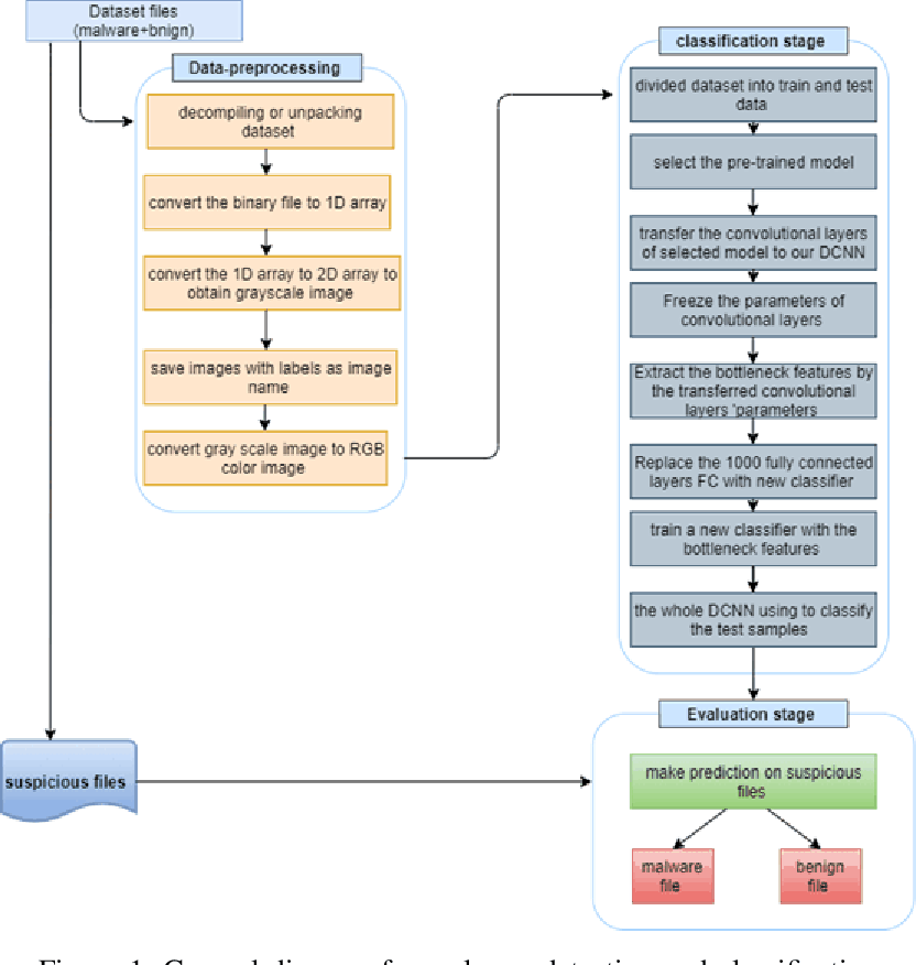
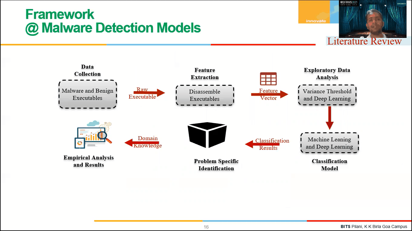
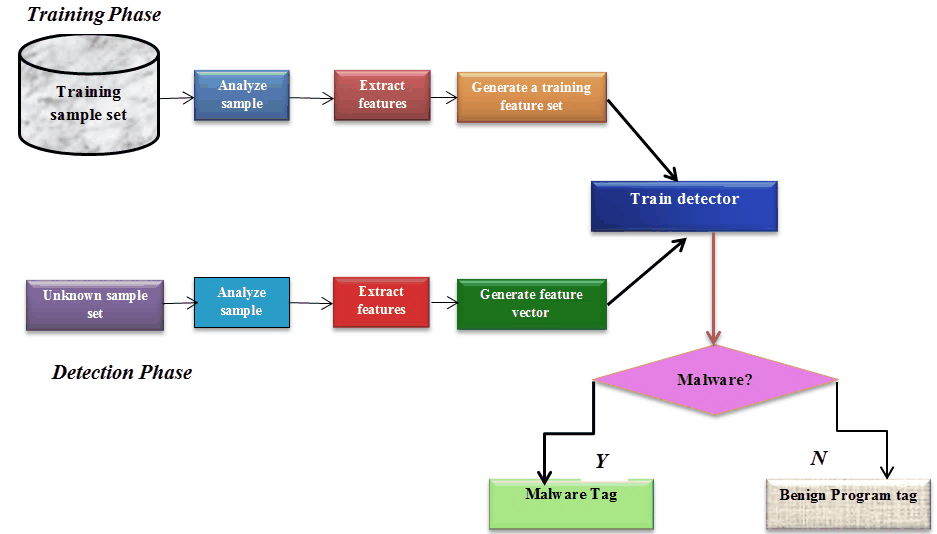
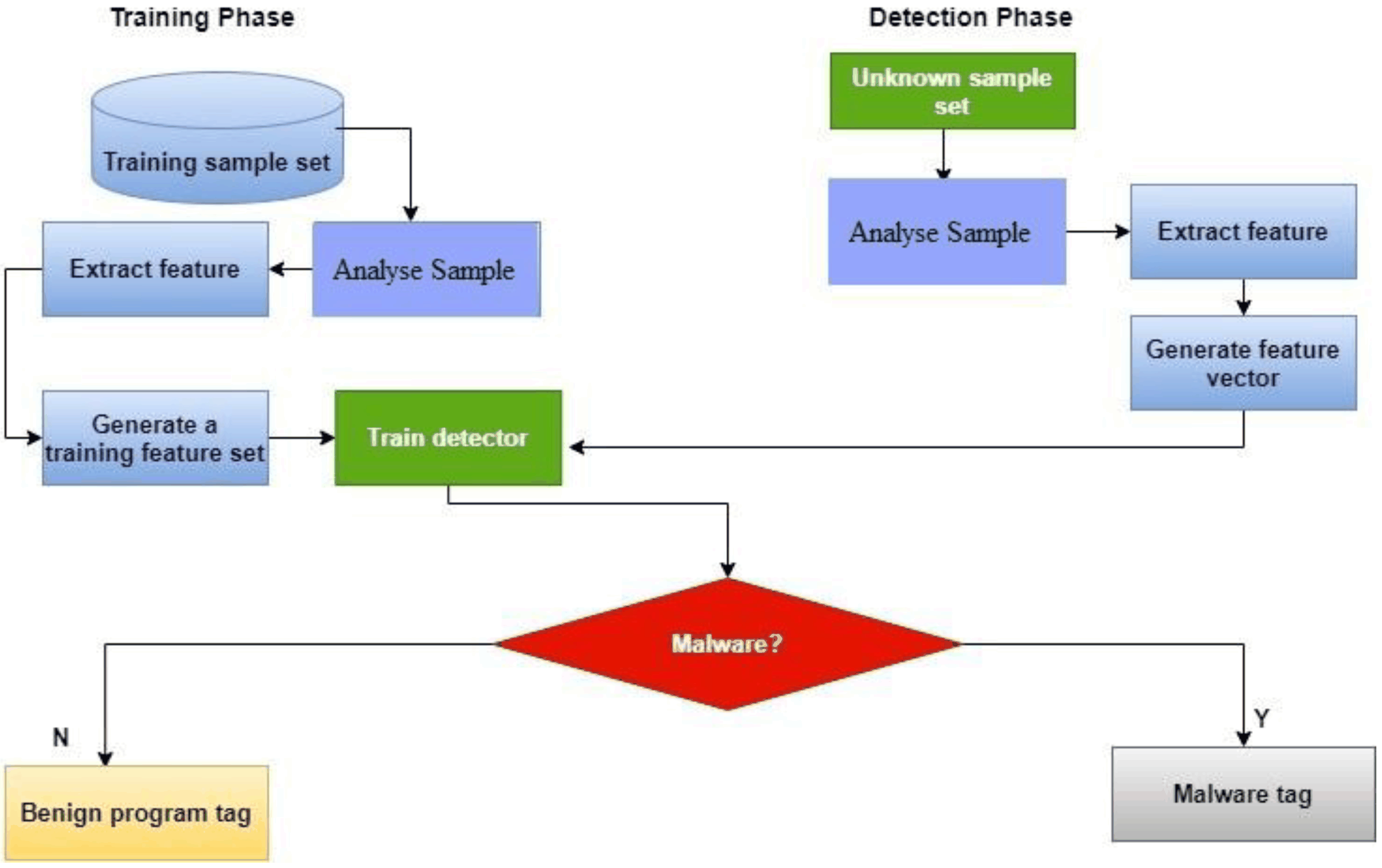
Deep Learning Execution Pipeline
(Preprocessing)
(Feature Extraction)
(Self-Attention)
(Loss Optimization)