Complete Technical Paper Content — Reinforcement Learning Projects
1. Executive Abstract, Problem Formulation & Background
Active learning is a special case of machine learning in which a learning algorithm can interactively query a human user (or some other information source) to label new data points with the desired outputs. The human user must possess expertise in the problem domain, including the ability to consult authoritative sources when necessary. In statistics literature, it is sometimes also called optimal experimental design. The information source is also called teacher or oracle. There are situations in which unlabeled data is abundant but manual labeling is expensive. In such a scenario, learning algorithms can actively query the teacher for labels. Since the learner chooses the examples, the number of examples to learn a concept can often be much lower than the number required in normal supervised learning. However, there is a risk that the algorithm is overwhelmed by uninformative examples. Recent developments are dedicated to multi-label active learning, hybrid active learning and active learning in a single-pass (on-line) context, combining concepts from the field of machine learning (e.g. conflict and ignorance) with adaptive, incremental learning policies in the field of online machine learning. Using active learning allows for faster development of a machine learning algorithm, when comparative updates would require a quantum or super computer. Large-scale active learning projects may benefit from crowdsourcing frameworks such as Amazon Mechanical Turk that include many humans in the active learning loop.
T K , i {\displaystyle \mathbf {T} _{K,i}} : Data points where the label is known.
T U , i {\displaystyle \mathbf {T} _{U,i}} : Data points where the label is unknown.
T C , i {\displaystyle \mathbf {T} _{C,i}} : A subset of TU,i that is chosen to be labeled. Most of the current research in active learning involves the best method to choose the data points for TC,i.
Balance exploration and exploitation: the choice of examples to label is seen as a dilemma between the exploration and the exploitation over the data space representation. This strategy manages this compromise by modelling the active learning problem as a contextual bandit problem. For example, Bouneffouf et al. propose a sequential algorithm named Active Thompson Sampling (ATS), which, in each round, assigns a sampling distribution on the pool, samples one point from this distribution, and queries the oracle for this sample point label. Expected model change: label those points that would most change the current model. Expected error reduction: label those points that would most reduce the model's generalization error. Exponentiated Gradient Exploration for Active Learning: In this paper, the author proposes a sequential algorithm named exponentiated gradient (EG)-active that can improve any active learning algorithm by an optimal random exploration. Uncertainty sampling: label those points for which the current model is least certain as to what the correct output should be. Query by committee: a variety of models are trained on the current labeled data, and vote on the output for unlabeled data; label those points for which the "committee" disagrees the most Querying from diverse subspaces or partitions: When the underlying model is a forest of trees, the leaf nodes might represent (overlapping) partitions of the original feature space. This offers the possibility of selecting instances from non-overlapping or minimally overlapping partitions for labeling. Variance reduction: label those points that would minimize output variance, which is one of the components of error. Conformal prediction: predicts that a new data point will have a label similar to old data points in some specified way and degree of the similarity within the old examples is used to estimate the confidence in the prediction. Mismatch-first farthest-traversal: The primary selection criterion is the prediction mismatch between the current model and nearest-neighbour prediction. It targets on wrongly predicted data points. The second selection criterion is the distance to previously selected data, the farthest first. It aims at optimizing the diversity of selected data. User-centered labeling strategies: Learning is accomplished by applying dimensionality reduction to graphs and figures like scatter plots. Then the user is asked to label the compiled data (categorical, numerical, relevance scores, relation between two instances). A wide variety of algorithms have been studied that fall into these categories. While the traditional AL strategies can achieve remarkable performance, it is often challenging to predict in advance which strategy is the most suitable in a particular situation. In recent years, meta-learning algorithms have been gaining in popularity. Some of them have been proposed to tackle the problem of learning AL strategies instead of relying on manually designed strategies. A benchmark which compares 'meta-learning approaches to active learning' to 'traditional heuristic-based Active Learning' may give intuitions if 'Learning active learning' is at the crossroads
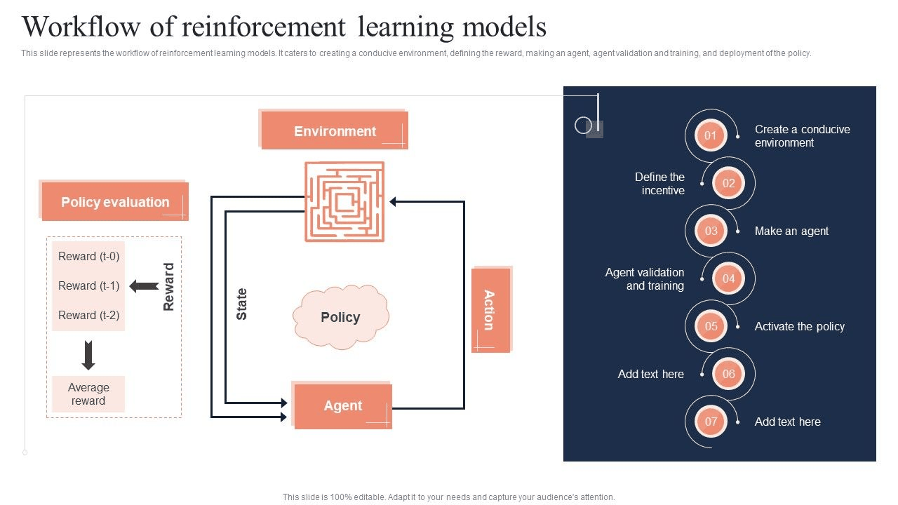
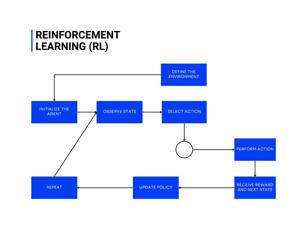
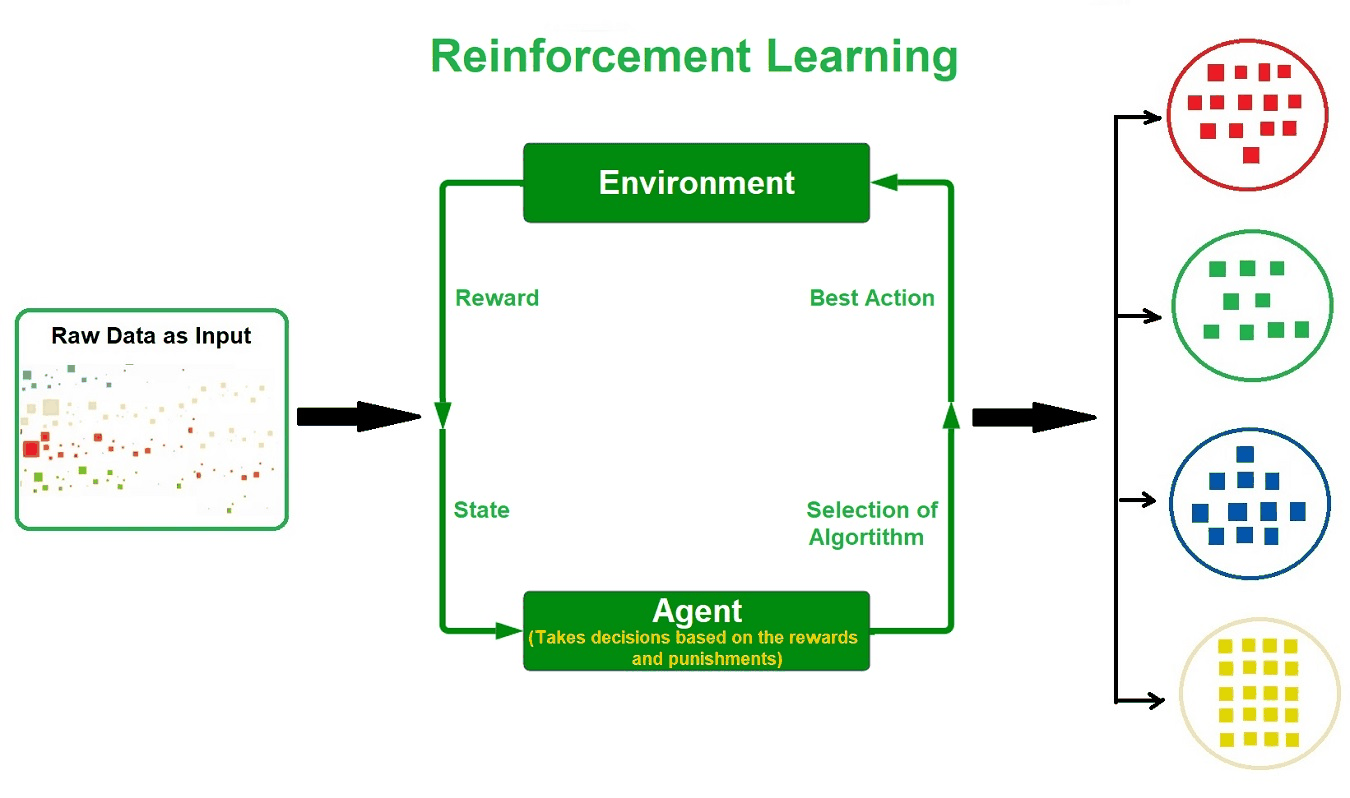
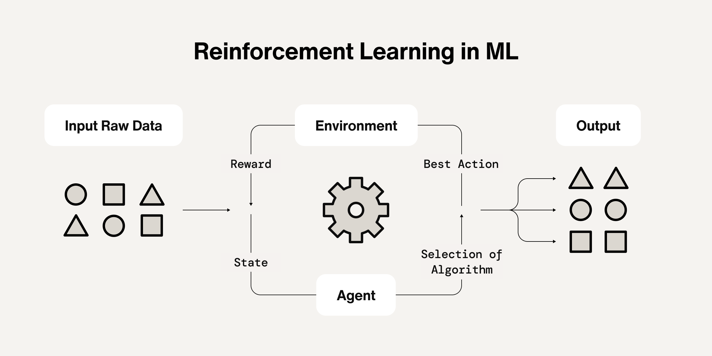
In machine learning and optimal control, reinforcement learning (RL) (also known as approximate dynamic programming) is concerned with how an intelligent agent should take actions in a dynamic environment in order to maximize a reward signal. Reinforcement learning is one of the three basic machine learning paradigms, alongside supervised learning and unsupervised learning. While supervised learning and unsupervised learning algorithms respectively attempt to discover patterns in labeled and unlabeled data, reinforcement learning involves training an agent through interactions with its environment. To learn to maximize rewards from these interactions, the agent makes decisions between trying new actions to learn more about the environment (exploration), or using current knowledge of the environment to take the best action (exploitation). The search for the optimal balance between these two strategies is known as the exploration–exploitation dilemma.
2. Related Work, Literature Survey & Algorithmic Foundations
The environment is typically stated in the form of a Markov decision process, as many reinforcement learning algorithms use dynamic programming techniques. The main difference between classical dynamic programming methods and reinforcement learning algorithms is that the latter do not assume knowledge of an exact mathematical model of the Markov decision process, and they target large Markov decision processes where exact methods become infeasible.
A set of environment and agent states (the state space), S {\displaystyle {\mathcal {S}}} ; A set of actions (the action space), A {\displaystyle {\mathcal {A}}} , of the agent;
P a ( s , s ′ ) = Pr ( S t + 1 = s ′ ∣ S t = s , A t = a ) {\displaystyle P_{a}(s,s')=\Pr(S_{t+1}{=}s'\mid S_{t}{=}s,A_{t}{=}a)} , the transition probability (at time t {\displaystyle t} ) from state s {\displaystyle s} to state s ′ {\displaystyle s'} under action a {\displaystyle a} .
R a ( s , s ′ ) {\displaystyle R_{a}(s,s')} , the immediate reward after transitioning from s {\displaystyle s} to s ′ {\displaystyle s'} under action a {\displaystyle a} . The purpose of reinforcement learning is for the agent to learn an optimal (or near-optimal) policy that maximizes the reward function or other user-provided reinforcement signal that accumulates from immediate rewards. This is similar to processes that appear to occur in animal psychology. For example, biological brains are hardwired to interpret signals such as pain and hunger as negative reinforcements, and interpret pleasure and food intake as positive reinforcements. In some circumstances, animals learn to adopt behaviors that optimize these rewards. This suggests that animals are capable of reinforcement learning. A basic reinforcement learning agent interacts with its environment in discrete time steps. At each time step t, the agent receives the current state S t {\displaystyle S_{t}} and reward R t {\displaystyle R_{t}} . It then chooses an action A t {\displaystyle A_{t}} from the set of available actions, which is subsequently sent to the environment. The environment moves to a new state S t + 1 {\displaystyle S_{t+1}} and the reward R t + 1 {\displaystyle R_{t+1}} associated with the transition ( S t , A t , S t + 1 ) {\displaystyle (S_{t},A_{t},S_{t+1})} is determined. The goal of a reinforcement learning agent is to learn a policy:
π : S × A → [ 0 , 1 ] π ( s , a ) = Pr ( A t = a ∣ S t = s ) {\displaystyle {\begin{aligned}&\pi :{\mathcal {S}}\times {\mathcal {A}}\to [0,1]\\&\pi (s,a)=\Pr(A_{t}{=}a\mid S_{t}{=}s)\end{aligned}}}
that maximizes the expected cumulative reward. Formulating the problem as a Markov decision process assumes the agent directly observes the current environmental state; in this case, the problem is said to have full observability. If the agent only has access to a subset of states, or if the observed states are corrupted by noise, the agent is said to have partial observability, and formally the problem must be formulated as a partially observable Markov decision process. In both cases, the set of actions available to the agent can be restricted. For example, the state of an account balance could be restricted to be positive; if the current value of the state is 3 and the state transition attempts to reduce the value by 4, the transition will not be allowed. When the agent's performance is compared to that of an agent that acts optimally, the difference in performance yields the notion of regret. In order to act near optimally, the agent must reason about long-term consequences of its actions (i.e., maximize future rewards), although the immediate reward associated with this might be negative. Thus, reinforcement learning is particularly well-suited to problems that include a long-term versus short-term reward trade-off. It has been applied successfully to various problems, including energy storage, robot control, photovoltaic generators, backgammon, checkers, Go (AlphaGo), and autonomous driving systems. Two elements make reinforcement learning powerful: the use of samples to optimize performance, and the use of function approximation to deal with large environments. Thanks to these two key components, RL can be used in large environments in the following situations:
3. Dataset Ingestion, Preprocessing & Stochastic Augmentations
A model of the environment is known, but an analytic solution is not available; Only a simulation model of the environment is given (the subject of simulation-based optimization); The only way to collect information about the environment is to interact with it. The first two of these problems could be considered planning problems (since some form of model is available), while the last one could be considered to be a genuine learning problem. However, reinforcement learning converts both planning problems to machine learning problems.
π : A × S → [ 0 , 1 ] π ( a , s ) = Pr ( A t = a ∣ S t = s ) {\displaystyle {\begin{aligned}&\pi :{\mathcal {A}}\times {\mathcal {S}}\to [0,1]\\&\pi (a,s)=\Pr(A_{t}{=}a\mid S_{t}{=}s)\end{aligned}}}
The policy map gives the probability of taking action a {\displaystyle a} when in state s {\displaystyle s} . There are also deterministic policies π {\displaystyle \pi } for which π ( s ) {\displaystyle \pi (s)} denotes the action that should be played at state s {\displaystyle s} .
V π ( s ) = E [ G ∣ S 0 = s ] = E [ ∑ t = 0 ∞ γ t R t + 1 ∣ S 0 = s ] , {\displaystyle V_{\pi }(s)=\operatorname {\mathbb {E} } [G\mid S_{0}{=}s]=\operatorname {\mathbb {E} } \left[\sum _{t=0}^{\infty }\gamma ^{t}R_{t+1}\mid S_{0}{=}s\right],}
where the random variable G {\displaystyle G} denotes the discounted return, and is defined as the sum of future discounted rewards:
G = ∑ t = 0 ∞ γ t R t + 1 = R 1 + γ R 2 + γ 2 R 3 + ⋯ , {\displaystyle G=\sum _{t=0}^{\infty }\gamma ^{t}R_{t+1}=R_{1}+\gamma R_{2}+\gamma ^{2}R_{3}+\cdots ,}
4. Neural Network Backbone, Layer Specifications & Loss Formulations
where R t + 1 {\displaystyle R_{t+1}} is the reward for transitioning from state S t {\displaystyle S_{t}} to S t + 1 {\displaystyle S_{t+1}} , 0 ≤ γ < 1 {\displaystyle 0\leq \gamma <1} is the discount rate. γ {\displaystyle \gamma } is less than 1, so rewards in the distant future are weighted less than rewards in the immediate future. The goal is to find a policy that maximizes the expected discounted return. From the theory of Markov decision processes it is known that, without loss of generality, the search can be restricted to the set of so-called stationary policies. A policy is stationary if the action-distribution returned by it depends only on the last state visited (from the observation agent's history). The search can be further restricted to deterministic stationary policies. A deterministic stationary policy deterministically selects actions based on the current state. Since any such policy can be identified with a mapping from the set of states to the set of actions, these policies can be identified with such mappings with no loss of generality.
For each possible policy, sample returns while following it Choose the policy with the largest expected discounted return One problem with this is that the number of policies can be large, or even infinite. Another is that the variance of the returns may be large, which requires many samples to accurately estimate the discounted return of each policy. These problems can be ameliorated if we assume some structure and allow samples generated from one policy to influence the estimates made for others. The two main approaches for achieving this are value function estimation and direct policy search.
Value function approaches attempt to find a policy that maximizes the discounted return by maintaining a set of estimates of expected discounted returns E [ G ] {\displaystyle \operatorname {\mathbb {E} } [G]} for some policy (usually either the "current" [on-policy] or the optimal [off-policy] one). These methods rely on the theory of Markov decision processes, where optimality is defined in a sense stronger than the one above: A policy is optimal if it achieves the best-expected discounted return from any initial state (i.e., initial distributions play no role in this definition). Again, an optimal policy can always be found among stationary policies. To define optimality in a formal manner, define the state-value of a policy π {\displaystyle \pi } by
V π ( s ) = E [ G ∣ s , π ] , {\displaystyle V^{\pi }(s)=\operatorname {\mathbb {E} } [G\mid s,\pi ],}
where G {\displaystyle G} stands for the discounted return associated with following π {\displaystyle \pi } from the initial state s {\displaystyle s} . Defining V ∗ ( s ) {\displaystyle V^{*}(s)} as the maximum possible state-value of V π ( s ) {\displaystyle V^{\pi }(s)} , where π {\displaystyle \pi } is allowed to change,
V ∗ ( s ) = max π V π ( s ) . {\displaystyle V^{*}(s)=\max _{\pi }V^{\pi }(s).}
5. Training Protocol, Convergence Behavior & Experimental Evaluation
A policy that achieves these optimal state-values in each state is called optimal. Clearly, a policy that is optimal in this sense is also optimal in the sense that it maximizes the expected discounted return, since V ∗ ( s ) = max π E [ G ∣ s , π ] {\displaystyle V^{*}(s)=\max _{\pi }\mathbb {E} [G\mid s,\pi ]} , where s {\displaystyle s} is a state randomly sampled from the distribution μ {\displaystyle \mu } of initial states (so μ ( s ) = Pr ( S 0 = s ) {\displaystyle \mu (s)=\Pr(S_{0}=s)} ). Although state-values suffice to define optimality, it is useful to define action-values. Given a state s {\displaystyle s} , an action a {\displaystyle a} and a policy π {\displaystyle \pi } , the action-value of the pair ( s , a ) {\displaystyle (s,a)} under π {\displaystyle \pi } is defined by
Q π ( s , a ) = E [ G ∣ s , a , π ] , {\displaystyle Q^{\pi }(s,a)=\operatorname {\mathbb {E} } [G\mid s,a,\pi ],}
where G {\displaystyle G} now stands for the random discounted return associated with first taking action a {\displaystyle a} in state s {\displaystyle s} and following π {\displaystyle \pi } , thereafter. The theory of Markov decision processes states that if π ∗ {\displaystyle \pi ^{*}} is an optimal policy, we act optimally (take the optimal action) by choosing the action from Q π ∗ ( s , ⋅ ) {\displaystyle Q^{\pi ^{*}}(s,\cdot )} with the highest action-value at each state, s {\displaystyle s} . The action-value function of such an optimal policy ( Q π ∗ {\displaystyle Q^{\pi ^{*}}} ) is called the optimal action-value function and is commonly denoted by Q ∗ {\displaystyle Q^{*}} . In summary, the knowledge of the optimal action-value function alone suffices to know how to act optimally. Assuming full knowledge of the Markov decision process, the two basic approaches to compute the optimal action-value function are value iteration and policy iteration. Both algorithms compute a sequence of functions Q k {\displaystyle Q_{k}} ( k = 0 , 1 , 2 , … {\displaystyle k=0,1,2,\ldots } ) that converge to Q ∗ {\displaystyle Q^{*}} . Computing these functions involves computing expectations over the whole state-space, which is impractical for all but the smallest (finite) Markov decision processes. In reinforcement learning methods, expectations are approximated by averaging over samples and using function approximation techniques to cope with the need to represent value functions over large state-action spaces.
The first problem is corrected by allowing the procedure to change the policy (at some or all states) before the values settle. This too may be problematic as it might prevent convergence. Most current algorithms do this, giving rise to the class of generalized policy iteration algorithms. Many actor-critic methods belong to this category. The second issue can be corrected by allowing trajectories to contribute to any state-action pair in them. This may also help to some extent with the third problem, although a better solution when returns have high variance is Sutton's temporal difference (TD) methods that are based on the recursive Bellman equation. The computation in TD methods can be incremental (when after each transition the memory is changed and the transition is thrown away), or batch (when the transitions are batched and the estimates are computed once based on the batch). Batch methods, such as the least-squares temporal difference method, may use the information in the samples better, while incremental methods are the only choice when batch methods are infeasible due to their high computational or memory complexity. Some methods try to combine the two approaches. Methods based on temporal differences also overcome the fourth issue. Another problem specific to TD comes from their reliance on the recursive Bellman equation. Most TD methods have a so-called λ {\displaystyle \lambda } parameter ( 0 ≤ λ ≤ 1 ) {\displaystyle (0\leq \lambda \leq 1)} that can continuously interpolate between Monte Carlo methods that do not rely on the Bellman equations and the basic TD methods that rely entirely on the Bellman equations. This can mitigate this issue.
Q ( s , a ) = ∑ i = 1 d θ i ϕ i ( s , a ) . {\displaystyle Q(s,a)=\sum _{i=1}^{d}\theta _{i}\phi _{i}(s,a).}
The algorithms then adjust the weights, instead of adjusting the values associated with the individual state-action pairs. Methods based on ideas from nonparametric statistics (which can be seen to construct their own features) have been explored. Value iteration can also be used as a starting point, giving rise to the Q-learning algorithm and its many variants. Including Deep Q-learning methods when a neural network is used to represent Q, with various applications in stochastic search problems. The problem with using action-values is that they may need highly precise estimates of the competing action values that can be hard to obtain when the returns are noisy, though this problem is mitigated to some extent by temporal difference methods. Using the so-called compatible function approximation method compromises generality and efficiency.
Model Figures & Evaluation Curves (4 Images)
Deep Learning Execution Pipeline
(Preprocessing)
(Feature Extraction)
(Self-Attention)
(Loss Optimization)