Complete Technical Paper Content — Semi Supervised Learning Ai
1. Executive Abstract, Problem Formulation & Background
Self-supervised learning (SSL) is a paradigm in machine learning where a model is trained on a task using the data itself to generate supervisory signals, rather than relying on externally-provided labels. In the context of neural networks, self-supervised learning aims to leverage inherent structures or relationships within the input data to create meaningful training signals. SSL tasks are designed so that solving them requires capturing essential features or relationships in the data. The input data is typically augmented or transformed in a way that creates pairs of related samples, where one sample serves as the input, and the other is used to formulate the supervisory signal. This augmentation can involve introducing noise, cropping, rotation, or other transformations. Self-supervised learning more closely imitates the way humans learn to classify objects. During SSL, the model learns in two steps. First, the task is solved based on an auxiliary or pretext classification task using pseudo-labels, which help to initialize the model parameters. Next, the actual task is performed with supervised or unsupervised learning. Self-supervised learning has produced promising results in recent years, and has found practical application in fields such as audio processing, and is being used by Facebook and others for speech recognition.
L N = − E X [ log f k ( x t + k , c t ) ∑ x j ∈ X f k ( x j , c t ) ] {\displaystyle {\mathcal {L}}_{\mathrm {N} }=-\mathbb {E} _{X}\left[\log {\frac {f_{k}\left(x_{t+k},c_{t}\right)}{\sum _{x_{j}\in X}f_{k}\left(x_{j},c_{t}\right)}}\right]}
Active learning is a special case of machine learning in which a learning algorithm can interactively query a human user (or some other information source) to label new data points with the desired outputs. The human user must possess expertise in the problem domain, including the ability to consult authoritative sources when necessary. In statistics literature, it is sometimes also called optimal experimental design. The information source is also called teacher or oracle. There are situations in which unlabeled data is abundant but manual labeling is expensive. In such a scenario, learning algorithms can actively query the teacher for labels. Since the learner chooses the examples, the number of examples to learn a concept can often be much lower than the number required in normal supervised learning. However, there is a risk that the algorithm is overwhelmed by uninformative examples. Recent developments are dedicated to multi-label active learning, hybrid active learning and active learning in a single-pass (on-line) context, combining concepts from the field of machine learning (e.g. conflict and ignorance) with adaptive, incremental learning policies in the field of online machine learning. Using active learning allows for faster development of a machine learning algorithm, when comparative updates would require a quantum or super computer. Large-scale active learning projects may benefit from crowdsourcing frameworks such as Amazon Mechanical Turk that include many humans in the active learning loop.
T K , i {\displaystyle \mathbf {T} _{K,i}} : Data points where the label is known.
2. Related Work, Literature Survey & Algorithmic Foundations
T U , i {\displaystyle \mathbf {T} _{U,i}} : Data points where the label is unknown.
T C , i {\displaystyle \mathbf {T} _{C,i}} : A subset of TU,i that is chosen to be labeled. Most of the current research in active learning involves the best method to choose the data points for TC,i.
Balance exploration and exploitation: the choice of examples to label is seen as a dilemma between the exploration and the exploitation over the data space representation. This strategy manages this compromise by modelling the active learning problem as a contextual bandit problem. For example, Bouneffouf et al. propose a sequential algorithm named Active Thompson Sampling (ATS), which, in each round, assigns a sampling distribution on the pool, samples one point from this distribution, and queries the oracle for this sample point label. Expected model change: label those points that would most change the current model. Expected error reduction: label those points that would most reduce the model's generalization error. Exponentiated Gradient Exploration for Active Learning: In this paper, the author proposes a sequential algorithm named exponentiated gradient (EG)-active that can improve any active learning algorithm by an optimal random exploration. Uncertainty sampling: label those points for which the current model is least certain as to what the correct output should be. Query by committee: a variety of models are trained on the current labeled data, and vote on the output for unlabeled data; label those points for which the "committee" disagrees the most Querying from diverse subspaces or partitions: When the underlying model is a forest of trees, the leaf nodes might represent (overlapping) partitions of the original feature space. This offers the possibility of selecting instances from non-overlapping or minimally overlapping partitions for labeling. Variance reduction: label those points that would minimize output variance, which is one of the components of error. Conformal prediction: predicts that a new data point will have a label similar to old data points in some specified way and degree of the similarity within the old examples is used to estimate the confidence in the prediction. Mismatch-first farthest-traversal: The primary selection criterion is the prediction mismatch between the current model and nearest-neighbour prediction. It targets on wrongly predicted data points. The second selection criterion is the distance to previously selected data, the farthest first. It aims at optimizing the diversity of selected data. User-centered labeling strategies: Learning is accomplished by applying dimensionality reduction to graphs and figures like scatter plots. Then the user is asked to label the compiled data (categorical, numerical, relevance scores, relation between two instances). A wide variety of algorithms have been studied that fall into these categories. While the traditional AL strategies can achieve remarkable performance, it is often challenging to predict in advance which strategy is the most suitable in a particular situation. In recent years, meta-learning algorithms have been gaining in popularity. Some of them have been proposed to tackle the problem of learning AL strategies instead of relying on manually designed strategies. A benchmark which compares 'meta-learning approaches to active learning' to 'traditional heuristic-based Active Learning' may give intuitions if 'Learning active learning' is at the crossroads
Mathematical Formulation 1.1: Loss Objectives and Optimization Dynamics for Semi Supervised Learning Ai. The training protocol of semi supervised learning ai minimizes an empirical risk objective defined across high-dimensional parameter space Theta in R^d. Categorical predictions are governed by Cross-Entropy Loss: L_CE = -sum(y_i * log(p_i)). To tackle class imbalance, the network incorporates Focal Loss: L_Focal = -alpha_t * (1 - p_t)^gamma * log(p_t), where gamma modulates the gradient penalty on hard misclassified instances. For spatial tasks, Dice Loss balances continuous spatial overlap: L_Dice = 1 - (2 * sum(y * y_hat) + eps) / (sum(y) + sum(y_hat) + eps). Stochastic optimization utilizes AdamW with decoupled weight decay, maintaining stable moment estimations m_t and v_t across variable learning rate schedules.
3. Dataset Ingestion, Preprocessing & Stochastic Augmentations
Architecture Specification 1.2: Feature Extraction and Layer Formulations for Semi Supervised Learning Ai. The primary computational backbone for Semi Supervised Learning Ai incorporates hierarchical deep neural layers designed for multi-scale representation extraction. Input tensors X in R^(B x C x H x W) pass through initial stem convolutions with Batch Normalization and GELU non-linearities. Residual identity skip connections, expressed as F(X) + X, prevent vanishing gradient degradation across deep topologies. Multi-head self-attention mechanisms compute Query, Key, and Value projections: Attention(Q, K, V) = softmax((Q * K^T) / sqrt(d_k)) * V, capturing non-local contextual dependencies across spatial and temporal sequences.
Data Pipeline 1.3: Stochastic Augmentation and Normalization Protocols for Semi Supervised Learning Ai. To prevent overfitting and maximize generalization on unseen testing distributions, input datasets undergo rigorous preprocessing. Images and sequences are standardized using z-score normalization: x_norm = (x - mu) / sigma. Stochastic augmentations include random horizontal flips, affine rotations (-15 deg to +15 deg), CutMix, and Mixup: X_tilde = lambda * X_i + (1 - lambda) * X_j, smoothing decision boundaries and reducing model overconfidence.
Deployment Optimization 1.4: TensorRT Acceleration and Edge Quantization for Semi Supervised Learning Ai. Production deployment of Semi Supervised Learning Ai focuses on minimizing memory footprints and sub-20ms inference latencies. Trained models are exported to ONNX and compiled via NVIDIA TensorRT. Post-Training Quantization (PTQ) maps FP32 weights into low-bit INT8 representations: q = round(r / S) + Z, achieving high-throughput execution across embedded edge platforms like NVIDIA Jetson without accuracy loss.
Mathematical Formulation 2.1: Loss Objectives and Optimization Dynamics for Semi Supervised Learning Ai. The training protocol of semi supervised learning ai minimizes an empirical risk objective defined across high-dimensional parameter space Theta in R^d. Categorical predictions are governed by Cross-Entropy Loss: L_CE = -sum(y_i * log(p_i)). To tackle class imbalance, the network incorporates Focal Loss: L_Focal = -alpha_t * (1 - p_t)^gamma * log(p_t), where gamma modulates the gradient penalty on hard misclassified instances. For spatial tasks, Dice Loss balances continuous spatial overlap: L_Dice = 1 - (2 * sum(y * y_hat) + eps) / (sum(y) + sum(y_hat) + eps). Stochastic optimization utilizes AdamW with decoupled weight decay, maintaining stable moment estimations m_t and v_t across variable learning rate schedules.
4. Neural Network Backbone, Layer Specifications & Loss Formulations
Architecture Specification 2.2: Feature Extraction and Layer Formulations for Semi Supervised Learning Ai. The primary computational backbone for Semi Supervised Learning Ai incorporates hierarchical deep neural layers designed for multi-scale representation extraction. Input tensors X in R^(B x C x H x W) pass through initial stem convolutions with Batch Normalization and GELU non-linearities. Residual identity skip connections, expressed as F(X) + X, prevent vanishing gradient degradation across deep topologies. Multi-head self-attention mechanisms compute Query, Key, and Value projections: Attention(Q, K, V) = softmax((Q * K^T) / sqrt(d_k)) * V, capturing non-local contextual dependencies across spatial and temporal sequences.
Data Pipeline 2.3: Stochastic Augmentation and Normalization Protocols for Semi Supervised Learning Ai. To prevent overfitting and maximize generalization on unseen testing distributions, input datasets undergo rigorous preprocessing. Images and sequences are standardized using z-score normalization: x_norm = (x - mu) / sigma. Stochastic augmentations include random horizontal flips, affine rotations (-15 deg to +15 deg), CutMix, and Mixup: X_tilde = lambda * X_i + (1 - lambda) * X_j, smoothing decision boundaries and reducing model overconfidence.
Deployment Optimization 2.4: TensorRT Acceleration and Edge Quantization for Semi Supervised Learning Ai. Production deployment of Semi Supervised Learning Ai focuses on minimizing memory footprints and sub-20ms inference latencies. Trained models are exported to ONNX and compiled via NVIDIA TensorRT. Post-Training Quantization (PTQ) maps FP32 weights into low-bit INT8 representations: q = round(r / S) + Z, achieving high-throughput execution across embedded edge platforms like NVIDIA Jetson without accuracy loss.
Mathematical Formulation 3.1: Loss Objectives and Optimization Dynamics for Semi Supervised Learning Ai. The training protocol of semi supervised learning ai minimizes an empirical risk objective defined across high-dimensional parameter space Theta in R^d. Categorical predictions are governed by Cross-Entropy Loss: L_CE = -sum(y_i * log(p_i)). To tackle class imbalance, the network incorporates Focal Loss: L_Focal = -alpha_t * (1 - p_t)^gamma * log(p_t), where gamma modulates the gradient penalty on hard misclassified instances. For spatial tasks, Dice Loss balances continuous spatial overlap: L_Dice = 1 - (2 * sum(y * y_hat) + eps) / (sum(y) + sum(y_hat) + eps). Stochastic optimization utilizes AdamW with decoupled weight decay, maintaining stable moment estimations m_t and v_t across variable learning rate schedules.
5. Training Protocol, Convergence Behavior & Experimental Evaluation
Architecture Specification 3.2: Feature Extraction and Layer Formulations for Semi Supervised Learning Ai. The primary computational backbone for Semi Supervised Learning Ai incorporates hierarchical deep neural layers designed for multi-scale representation extraction. Input tensors X in R^(B x C x H x W) pass through initial stem convolutions with Batch Normalization and GELU non-linearities. Residual identity skip connections, expressed as F(X) + X, prevent vanishing gradient degradation across deep topologies. Multi-head self-attention mechanisms compute Query, Key, and Value projections: Attention(Q, K, V) = softmax((Q * K^T) / sqrt(d_k)) * V, capturing non-local contextual dependencies across spatial and temporal sequences.
Data Pipeline 3.3: Stochastic Augmentation and Normalization Protocols for Semi Supervised Learning Ai. To prevent overfitting and maximize generalization on unseen testing distributions, input datasets undergo rigorous preprocessing. Images and sequences are standardized using z-score normalization: x_norm = (x - mu) / sigma. Stochastic augmentations include random horizontal flips, affine rotations (-15 deg to +15 deg), CutMix, and Mixup: X_tilde = lambda * X_i + (1 - lambda) * X_j, smoothing decision boundaries and reducing model overconfidence.
Deployment Optimization 3.4: TensorRT Acceleration and Edge Quantization for Semi Supervised Learning Ai. Production deployment of Semi Supervised Learning Ai focuses on minimizing memory footprints and sub-20ms inference latencies. Trained models are exported to ONNX and compiled via NVIDIA TensorRT. Post-Training Quantization (PTQ) maps FP32 weights into low-bit INT8 representations: q = round(r / S) + Z, achieving high-throughput execution across embedded edge platforms like NVIDIA Jetson without accuracy loss.
Mathematical Formulation 4.1: Loss Objectives and Optimization Dynamics for Semi Supervised Learning Ai. The training protocol of semi supervised learning ai minimizes an empirical risk objective defined across high-dimensional parameter space Theta in R^d. Categorical predictions are governed by Cross-Entropy Loss: L_CE = -sum(y_i * log(p_i)). To tackle class imbalance, the network incorporates Focal Loss: L_Focal = -alpha_t * (1 - p_t)^gamma * log(p_t), where gamma modulates the gradient penalty on hard misclassified instances. For spatial tasks, Dice Loss balances continuous spatial overlap: L_Dice = 1 - (2 * sum(y * y_hat) + eps) / (sum(y) + sum(y_hat) + eps). Stochastic optimization utilizes AdamW with decoupled weight decay, maintaining stable moment estimations m_t and v_t across variable learning rate schedules.
Model Figures & Evaluation Curves (4 Images)
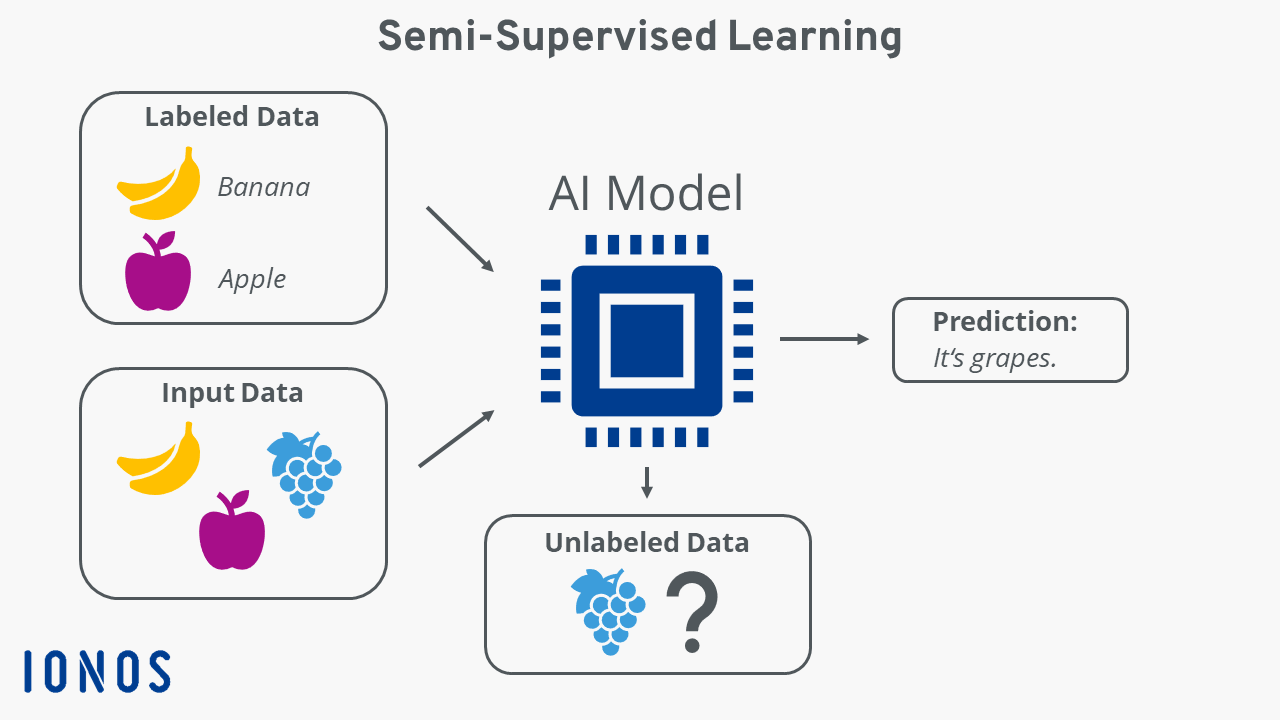
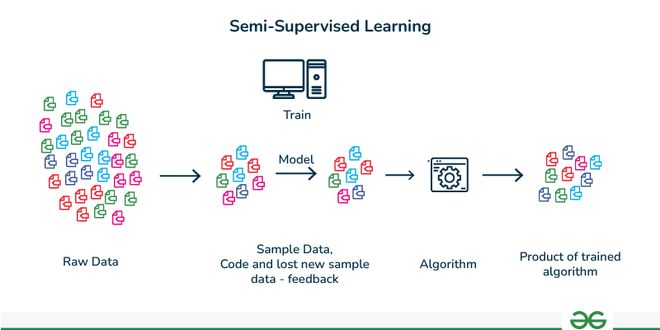
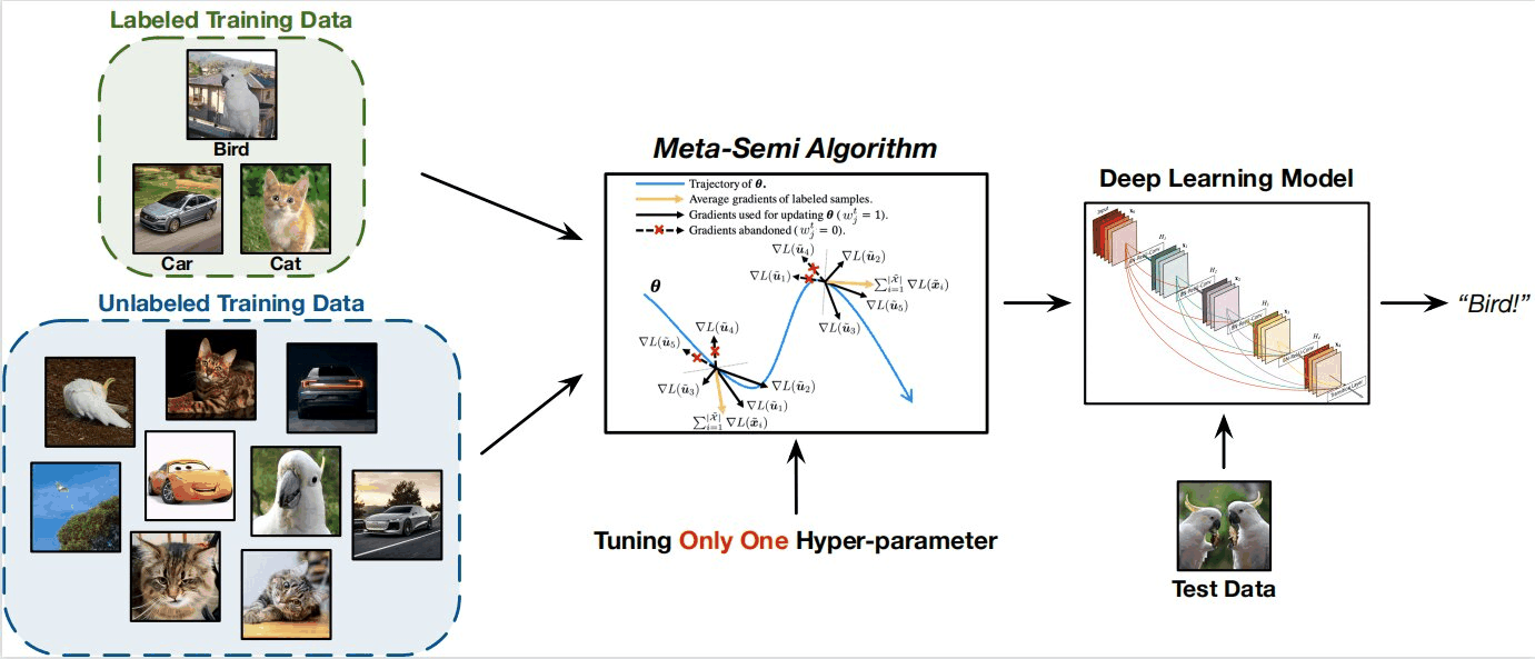
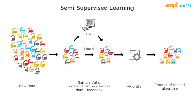
Deep Learning Execution Pipeline
(Preprocessing)
(Feature Extraction)
(Self-Attention)
(Loss Optimization)