Complete Technical Paper Content — Seq2Seq Models Projects
1. Executive Abstract, Problem Formulation & Background
In machine learning and natural language processing, seq2seq is a family of approaches that uses sequence transformation, i.e., it turns an input sequence into an output sequence. Originally developed by Lê Viết Quốc, a Vietnamese computer scientist and a machine learning pioneer at Google Brain, this framework has become foundational in many modern AI systems. Applications include language translation, image captioning, conversational models, speech recognition, and text summarization.
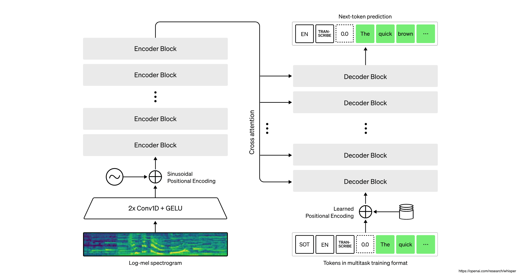
seq2seq is an approach to machine translation (or more generally, sequence transduction) with roots in information theory, where communication is understood as an encode-transmit-decode process, and machine translation can be studied as a special case of communication. This viewpoint was elaborated, for example, in the noisy channel model of machine translation. In practice, seq2seq maps an input sequence into a real-numerical vector by using a neural network (the encoder), and then maps it back to an output sequence using another neural network (the decoder). The idea of encoder-decoder sequence transduction had been developed in the early 2010s. The papers most commonly cited as the originators that produced seq2seq are two papers from 2014. In the seq2seq as proposed by them, both the encoder and the decoder were LSTMs. This had the "bottleneck" problem, since the encoding vector has a fixed size, so for long input sequences, information would tend to be lost, as they are difficult to fit into the fixed-length encoding vector. The attention mechanism, proposed in 2014, resolved the bottleneck problem. They called their model RNNsearch, as it "emulates searching through a source sentence during decoding a translation". A problem with seq2seq models at this point was that recurrent neural networks are difficult to parallelize. The 2017 publication of Transformers resolved the problem by replacing the encoding RNN with self-attention Transformer blocks ("encoder blocks"), and the decoding RNN with cross-attention causally-masked Transformer blocks ("decoder blocks").
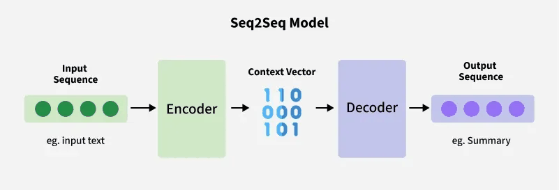
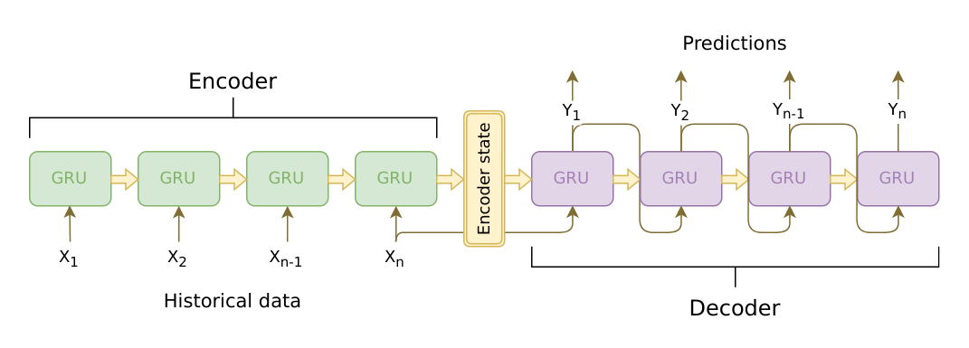
The encoder is responsible for processing the input sequence and capturing its essential information, which is stored as the hidden state of the network and, in a model with attention mechanism, a context vector. The context vector is the weighted sum of the input hidden states and is generated for every time instance in the output sequences.
The decoder takes the context vector and hidden states from the encoder and generates the final output sequence. The decoder operates in an autoregressive manner, producing one element of the output sequence at a time. At each step, it considers the previously generated elements, the context vector, and the input sequence information to make predictions for the next element in the output sequence. Specifically, in a model with attention mechanism, the context vector and the hidden state are concatenated together to form an attention hidden vector, which is used as an input for the decoder. The seq2seq method developed in the early 2010s uses two neural networks: an encoder network converts an input sentence into numerical vectors, and a decoder network converts those vectors to sentences in the target language. The Attention mechanism was grafted onto this structure in 2014 and is shown below. Later it was refined into the encoder-decoder Transformer architecture of 2017.
There is a subtle difference between training and prediction. During training time, both the input and the output sequences are known. During prediction time, only the input sequence is known, and the output sequence must be decoded by the network itself. Specifically, consider an input sequence x 1 : n {\displaystyle x_{1:n}} and output sequence y 1 : m {\displaystyle y_{1:m}} . The encoder would process the input x 1 : n {\displaystyle x_{1:n}} step by step. After that, the decoder would take the output from the encoder, as well as the <bos> as input, and produce a prediction y ^ 1 {\displaystyle {\hat {y}}_{1}} . Now, the question is: what should be input to the decoder in the next step? A standard method for training is "teacher forcing". In teacher forcing, no matter what is output by the decoder, the next input to the decoder is always the reference. That is, even if y ^ 1 ≠ y 1 {\displaystyle {\hat {y}}_{1}\neq y_{1}} , the next input to the decoder is still y 1 {\displaystyle y_{1}} , and so on. During prediction time, the "teacher" y 1 : m {\displaystyle y_{1:m}} would be unavailable. Therefore, the input to the decoder must be y ^ 1 {\displaystyle {\hat {y}}_{1}} , then y ^ 2 {\displaystyle {\hat {y}}_{2}} , and so on. It is found that if a model is trained purely by teacher forcing, its performance would degrade during prediction time, since generation based on the model's own output is different from generation based on the teacher's output. This is called exposure bias or a train/test distribution shift. A 2015 paper recommends that, during training, randomly switch between teacher forcing and no teacher forcing.
Consider the seq2seq language English-to-French translation task. To be concrete, let us consider the translation of "the zone of international control <end>", which should translate to "la zone de contrôle international <end>". Here, we use the special <end> token as a control character to delimit the end of input for both the encoder and the decoder. An input sequence of text x 0 , x 1 , … {\displaystyle x_{0},x_{1},\dots } is processed by a neural network (which can be an LSTM, a Transformer encoder, or some other network) into a sequence of real-valued vectors h 0 , h 1 , … {\displaystyle h_{0},h_{1},\dots } , where h {\displaystyle h} stands for "hidden vector". After the encoder has finished processing, the decoder starts operating over the hidden vectors, to produce an output sequence y 0 , y 1 , … {\displaystyle y_{0},y_{1},\dots } , autoregressively. That is, it always takes as input both the hidden vectors produced by the encoder, and what the decoder itself has produced before, to produce the next output word:
( h 0 , h 1 , … {\displaystyle h_{0},h_{1},\dots } , "<start>") → "la" ( h 0 , h 1 , … {\displaystyle h_{0},h_{1},\dots } , "<start> la") → "la zone" ( h 0 , h 1 , … {\displaystyle h_{0},h_{1},\dots } , "<start> la zone") → "la zone de" ... ( h 0 , h 1 , … {\displaystyle h_{0},h_{1},\dots } , "<start> la zone de contrôle international") → "la zone de contrôle international <end>" Here, we use the special <start> token as a control character to delimit the start of input for the decoder. The decoding terminates as soon as "<end>" appears in the decoder output.
2. Related Work, Literature Survey & Algorithmic Foundations
As hand-crafting weights defeats the purpose of machine learning, the model must compute the attention weights on its own. Taking analogy from the language of database queries, we make the model construct a triple of vectors: key, query, and value. The rough idea is that we have a "database" in the form of a list of key-value pairs. The decoder sends in a query, and obtains a reply in the form of a weighted sum of the values, where the weight is proportional to how closely the query resembles each key. The decoder first processes the "<start>" input partially, to obtain an intermediate vector h 0 d {\displaystyle h_{0}^{d}} , the 0th hidden vector of decoder. Then, the intermediate vector is transformed by a linear map W Q {\displaystyle W^{Q}} into a query vector q 0 = h 0 d W Q {\displaystyle q_{0}=h_{0}^{d}W^{Q}} . Meanwhile, the hidden vectors outputted by the encoder are transformed by another linear map W K {\displaystyle W^{K}} into key vectors k 0 = h 0 W K , k 1 = h 1 W K , … {\displaystyle k_{0}=h_{0}W^{K},k_{1}=h_{1}W^{K},\dots } . The linear maps are useful for providing the model with enough freedom to find the best way to represent the data. Now, the query and keys are compared by taking dot products: q 0 k 0 T , q 0 k 1 T , … {\displaystyle q_{0}k_{0}^{T},q_{0}k_{1}^{T},\dots } . Ideally, the model should have learned to compute the keys and values, such that q 0 k 0 T {\displaystyle q_{0}k_{0}^{T}} is large, q 0 k 1 T {\displaystyle q_{0}k_{1}^{T}} is small, and the rest are very small. This can be interpreted as saying that the attention weight should be mostly applied to the 0th hidden vector of the encoder, a little to the 1st, and essentially none to the rest. In order to make a properly weighted sum, we need to transform this list of dot products into a probability distribution over 0 , 1 , … {\displaystyle 0,1,\dots } . This can be accomplished by the softmax function, thus giving us the attention weights: ( w 00 , w 01 , … ) = s o f t m a x ( q 0 k 0 T , q 0 k 1 T , … ) {\displaystyle (w_{00},w_{01},\dots )=\mathrm {softmax} (q_{0}k_{0}^{T},q_{0}k_{1}^{T},\dots )} This is then used to compute the context vector: c 0 = w 00 v 0 + w 01 v 1 + ⋯ {\displaystyle c_{0}=w_{00}v_{0}+w_{01}v_{1}+\cdots }
where v 0 = h 0 W V , v 1 = h 1 W V , … {\displaystyle v_{0}=h_{0}W^{V},v_{1}=h_{1}W^{V},\dots } are the value vectors, linearly transformed by another matrix to provide the model with freedom to find the best way to represent values. Without the matrices W Q , W K , W V {\displaystyle W^{Q},W^{K},W^{V}} , the model would be forced to use the same hidden vector for both key and value, which might not be appropriate, as these two tasks are not the same.
This is the dot-attention mechanism. The particular version described in this section is "decoder cross-attention", as the output context vector is used by the decoder, and the input keys and values come from the encoder, but the query comes from the decoder, thus "cross-attention".
More succinctly, we can write it as c 0 = A t t e n t i o n ( h 0 d W Q , H W K , H W V ) = s o f t m a x ( ( h 0 d W Q ) ( H W K ) T ) ( H W V ) {\displaystyle c_{0}=\mathrm {Attention} (h_{0}^{d}W^{Q},HW^{K},HW^{V})=\mathrm {softmax} ((h_{0}^{d}W^{Q})\;(HW^{K})^{T})(HW^{V})} where the matrix H {\displaystyle H} is the matrix whose rows are h 0 , h 1 , … {\displaystyle h_{0},h_{1},\dots } . Note that the querying vector, h 0 d {\displaystyle h_{0}^{d}} , is not necessarily the same as the key-value vector h 0 {\displaystyle h_{0}} . In fact, it is theoretically possible for query, key, and value vectors to all be different, though that is rarely done in practice.
In machine learning, attention is a method that determines the importance of, or "attends to", each component in a sequence relative to the other components in that sequence. In natural language processing, importance is represented by "soft" weights assigned to each word in a sentence. More generally, attention encodes vectors called token embeddings across a fixed-width sequence that can range from tens to millions of tokens in size. Unlike "hard" weights, which are computed during the backwards training pass, "soft" weights exist only in the forward pass and therefore change with every step of the input. Earlier designs implemented the attention mechanism in a serial recurrent neural network (RNN) language translation system, but a more recent design, namely the transformer, removed the slower sequential RNN and relied more heavily on the faster parallel attention scheme. Inspired by ideas about attention in humans, the attention mechanism was developed to address the weaknesses of using information from the hidden layers of recurrent neural networks. Recurrent neural networks favor information contained in words at the end of a sentence and thus deemed more recent, thereby tending to attenuate the significance and associated predictive weight assigned to information earlier in the sentence. Attention allows a token equal access to any part of a sentence directly, rather than only through the previous state.
Additional surveys of the attention mechanism in deep learning are provided by Niu et al. and Soydaner. The major breakthrough came with self-attention, where each element in the input sequence attends to all others, enabling the model to capture global dependencies. This idea was central to the Transformer architecture, which replaced recurrence with attention mechanisms. As a result, Transformers became the foundation for models like BERT, T5 and generative pre-trained transformers (GPT).
The modern era of machine attention was revitalized by grafting an attention mechanism (Fig 1. orange) to an Encoder-Decoder.
3. Dataset Ingestion, Preprocessing & Stochastic Augmentations
Sometimes, alignment can be multiple-to-multiple. For example, the English phrase look it up corresponds to cherchez-le. Thus, "soft" attention weights work better than "hard" attention weights (setting one attention weight to 1, and the others to 0), as we would like the model to make a context vector consisting of a weighted sum of the hidden vectors, rather than "the best one", as there may not be a best hidden vector.
fast weight programmers, or fast weight controllers (1992). A "slow" neural network outputs the "fast" weights of another neural network through outer products. The slow network learns by gradient descent. It was later renamed as "linearized self-attention". Bahdanau-style attention, also referred to as additive attention, Luong-style attention, which is known as multiplicative attention, Early attention mechanisms similar to modern self-attention were proposed using recurrent neural networks. However, the highly parallelizable self-attention was introduced in 2017 and successfully used in the Transformer model, positional attention and factorized positional attention. For convolutional neural networks, attention mechanisms can be distinguished by the dimension on which they operate, namely: spatial attention, channel attention, or combinations. These variants recombine the encoder-side inputs to redistribute those effects to each target output. Often, a correlation-style matrix of dot products provides the re-weighting coefficients. In the figures below, W is the matrix of context attention weights, similar to the formula in Overview section above.
From the original paper on vision transformers (ViT), visualizing attention scores as a heat map (called saliency maps or attention maps) has become an important and routine way to inspect the decision making process of ViT models. One can compute the attention maps with respect to any attention head at any layer, while the deeper layers tend to show more semantically meaningful visualization. Attention rollout is a recursive algorithm to combine attention scores across all layers, by computing the dot product of successive attention maps. Because vision transformers are typically trained in a self-supervised manner, attention maps are generally not class-sensitive. When a classification head is attached to the ViT backbone, class-discriminative attention maps (CDAM) combines attention maps and gradients with respect to the class [CLS] token. Some class-sensitive interpretability methods originally developed for convolutional neural networks can be also applied to ViT, such as GradCAM, which back-propagates the gradients to the outputs of the final attention layer. Using attention as basis of explanation for the transformers in language and vision is not without debate. While some pioneering papers analyzed and framed attention scores as explanations, higher attention scores do not always correlate with greater impact on model performances.
Attention ( Q , K , V ) = softmax ( Q K T d k ) V ∈ R m × d v {\displaystyle {\text{Attention}}(Q,K,V)={\text{softmax}}\left({\frac {QK^{T}}{\sqrt {d_{k}}}}\right)V\in \mathbb {R} ^{m\times d_{v}}}
T {\displaystyle {}^{T}} denotes transpose and the softmax function is applied independently to every row of its argument. The matrix Q {\displaystyle Q} contains m {\displaystyle m} queries, while matrices K , V {\displaystyle K,V} jointly contain an unordered set of n {\displaystyle n} key-value pairs. Value vectors in matrix V {\displaystyle V} are weighted using the weights resulting from the softmax operation, so that the rows of the m {\displaystyle m} -by- d v {\displaystyle d_{v}} output matrix are confined to the convex hull of the points in R d v {\displaystyle \mathbb {R} ^{d_{v}}} given by the rows of V {\displaystyle V} . To understand the permutation invariance and permutation equivariance properties of QKV attention, let A ∈ R m × m {\displaystyle A\in \mathbb {R} ^{m\times m}} and B ∈ R n × n {\displaystyle B\in \mathbb {R} ^{n\times n}} be permutation matrices; and D ∈ R m × n {\displaystyle D\in \mathbb {R} ^{m\times n}} an arbitrary matrix. The softmax function is permutation equivariant in the sense that:
softmax ( A D B ) = A softmax ( D ) B {\displaystyle {\text{softmax}}(ADB)=A\,{\text{softmax}}(D)B}
Attention ( A Q , B K , B V ) = A Attention ( Q , K , V ) {\displaystyle {\text{Attention}}(AQ,BK,BV)=A\,{\text{Attention}}(Q,K,V)}
4. Neural Network Backbone, Layer Specifications & Loss Formulations
which shows that QKV attention is equivariant with respect to re-ordering the queries (rows of Q {\displaystyle Q} ); and invariant to re-ordering of the key-value pairs in K , V {\displaystyle K,V} . These properties are inherited when applying linear transforms to the inputs and outputs of QKV attention blocks. For example, a simple self-attention function defined as:
X ↦ Attention ( X T q , X T k , X T v ) {\displaystyle X\mapsto {\text{Attention}}(XT_{q},XT_{k},XT_{v})} is permutation equivariant with respect to re-ordering the rows of the input matrix X {\displaystyle X} in a non-trivial way, because every row of the output is a function of all the rows of the input. Similar properties hold for multi-head attention, which is defined below.
Attention ( Q , K , V ) = softmax ( Q K T d k + M ) V {\displaystyle {\text{Attention}}(Q,K,V)={\text{softmax}}\left({\frac {QK^{T}}{\sqrt {d_{k}}}}+M\right)V}
where the mask, M ∈ { 0 , − ∞ } n × n {\displaystyle M\in \mathbb {\{0,-\infty \}} ^{n\times n}} is a strictly upper triangular matrix, with zeros on and below the diagonal and − ∞ {\displaystyle -\infty } in every element above the diagonal. The softmax output, in R n × n {\displaystyle \mathbb {R} ^{n\times n}} is then lower triangular, with zeros in all elements above the diagonal. The masking ensures that for all 1 ≤ i < j ≤ n {\displaystyle 1\leq i<j\leq n} , row i {\displaystyle i} of the attention output is independent of row j {\displaystyle j} of any of the three input matrices. The permutation invariance and equivariance properties of standard QKV attention do not hold for the masked variant.
MultiHead ( Q , K , V ) = Concat ( head 1 , . . . , head h ) W O {\displaystyle {\text{MultiHead}}(Q,K,V)={\text{Concat}}({\text{head}}_{1},...,{\text{head}}_{h})W^{O}}
head i = Attention ( Q W i Q , K W i K , V W i V ) {\displaystyle {\text{head}}_{i}={\text{Attention}}(QW_{i}^{Q},KW_{i}^{K},VW_{i}^{V})}
and W i Q , W i K , W i V {\displaystyle W_{i}^{Q},W_{i}^{K},W_{i}^{V}} , and W O {\displaystyle W^{O}} are parameter matrices. The permutation properties of (standard, unmasked) QKV attention apply here also. For permutation matrices, A , B {\displaystyle A,B} :
5. Training Protocol, Convergence Behavior & Experimental Evaluation
MultiHead ( A Q , B K , B V ) = A MultiHead ( Q , K , V ) {\displaystyle {\text{MultiHead}}(AQ,BK,BV)=A\,{\text{MultiHead}}(Q,K,V)}
X ↦ MultiHead ( X T q , X T k , X T v ) {\displaystyle X\mapsto {\text{MultiHead}}(XT_{q},XT_{k},XT_{v})} is equivariant with respect to re-ordering of the rows of input matrix X {\displaystyle X} .
Attention ( Q , K , V ) = softmax ( tanh ( W Q Q + W K K ) ) V {\displaystyle {\text{Attention}}(Q,K,V)={\text{softmax}}(\tanh(W_{Q}Q+W_{K}K))V}
where W Q {\displaystyle W_{Q}} and W K {\displaystyle W_{K}} are learnable weight matrices.
Attention ( Q , K , V ) = softmax ( Q W K T ) V {\displaystyle {\text{Attention}}(Q,K,V)={\text{softmax}}(QWK^{T})V}
where W {\displaystyle W} is a learnable weight matrix.
Seq2seq Sequence to Sequence Learning with Keras Hi! You have just found Seq2Seq. Seq2Seq is a sequence to sequence learning add-on for the python deep learning library Keras . Using Seq2Seq, you can build and train sequence-to-sequence neural network models in Keras. Such models are useful for machine translation, chatbots (see [4] ), parsers, or whatever that comes to your mind. Getting started Seq2Seq contains modular and reusable layers that you can use to build your own seq2seq models as well as built-in models that work out of the box. Seq2Seq models can be compiled as they are or added as layers to a bigger model. Every Seq2Seq model has 2 primary layers : the encoder and the decoder. Generally, the encoder encodes the input sequence to an internal representation called 'context vector' which is used by the decoder to generate the output sequence. The lengths of input and output sequences can be different, as there is no explicit one on one relation between the input and output sequences. In addition to the encoder and decoder layers, a Seq2Seq model may also contain layers such as the left-stack (Stacked LSTMs on the encoder side), the right-stack (Stacked LSTMs on the decoder side), resizers (for shape compatibility between the encoder and the decoder) and dropout layers to avoid overfitting. The source code is heavily documented, so lets go straight to the examples: A simple Seq2Seq model: import seq2seq from seq2seq . models import SimpleSeq2Seq model = SimpleSeq2Seq ( input_dim = 5 , hidden_dim = 10 , output_length = 8 , output_dim = 8 ) model . compile ( loss = 'mse' , optimizer = 'rmsprop' ) That's it! You have successfully compiled a minimal Seq2Seq model! Next, let's build a 6 layer deep Seq2Seq model (3 layers for encoding, 3 layers for decoding). Deep Seq2Seq models: import seq2seq from seq2seq . models import SimpleSeq2Seq model = SimpleSeq2Seq ( input_dim = 5 , hidden_dim = 10 , output_length = 8 , output_dim = 8 , depth = 3 ) model . compile ( loss = 'mse' , optimizer = 'rmsprop' ) Notice that we have specified the depth for both encoder and decoder as 3, and your model has a total depth of 3 + 3 = 6. You can also specify different depths for the encoder and the decoder. Example: import seq2seq from seq2seq . models import SimpleSeq2Seq model = SimpleSeq2Seq ( input_dim = 5 , hidden_dim = 10 , output_length = 8 , output_dim = 20 , depth = ( 4 , 5 )) model . compile ( loss = 'mse' , optimizer = 'rmsprop' ) Notice that the depth is specified as tuple, (4, 5) . Which means your encoder will be 4 layers deep whereas your decoder will be 5 layers deep. And your model will have a total depth of 4 + 5 = 9. Advanced Seq2Seq models: Until now, you have been using the SimpleSeq2Seq model, which is a very minimalistic model. In the actual Seq2Seq implementation described in [1] , the hidden state of the encoder is transferred to decoder. Also, the output of decoder at each timestep becomes the input to the decoder at the next time step. To make things more complicated, the hidden state is propogated throughout the LSTM stack. But you have no reason to worry, as we have a built-in model that does all that out of the box. Example: import seq2seq from seq2seq . models import Seq2Seq model = Seq2Seq ( batch_input_shape = ( 16 , 7 , 5 ), hidden_dim = 10 , output_length = 8 , output_dim = 20 , depth = 4 ) model . compile ( loss = 'mse' , optimizer = 'rmsprop' ) Note that we had to specify the complete input shape, including the samples dimensions. This is because we need a static hidden state(similar to a stateful RNN) for transferring it across layers. (Update : Full input shape is not required in the latest version, since we switched to Recurrent Shop backend). By the way, Seq2Seq models also support the stateful argument, in case you need it. You can also experiment with the hidden state propogation turned off. Simply set the arguments broadcast_state and inner_broadcast_state to False . Peeky Seq2seq model : Let's not stop there. Let's build a model similar to cho et al 2014 , where the decoder gets a 'peek' at the context vector at every timestep. To achieve this, simply add the argument peek=True : import seq2seq from seq2seq . models import Seq2Seq model = Seq2Seq ( batch_input_shape = ( 16 , 7 , 5 ), hidden_dim = 10 , output_length = 8 , output_dim = 20 , depth = 4 , peek = True ) model . compile ( loss = 'mse' , optimizer = 'rmsprop' ) Seq2seq model with attention: Let's not stop there either. In all the models described above, there is no allignment between the input sequence elements and the output sequence elements. But for machine translation, learning a soft allignment between the input and output sequences imporves performance. [3] . The Seq2seq framework includes a ready made attention model which does the same. Note that in the attention model, there is no hidden state propogation, and a bidirectional LSTM encoder is used by default. Example: import seq2seq from seq2seq . models import AttentionSeq2Seq model = AttentionSeq2Seq ( input_dim = 5 , input_length = 7 , hidden_dim = 10 , output_length = 8 , output_dim = 20 , depth = 4 ) model . compile ( loss = 'mse' , optimizer = 'rmsprop' ) As you can see, in the attention model you need not specify the samples dimension as there are no static hidden states involved(But you have to if you are building a stateful Seq2seq model). Note: You can set the argument bidirectional=False if you wish not to use a bidirectional encoder. Final Words That's all for now. Hope you love this library. For any questions you might have, create an issue and I will get in touch. You can also contribute to this project by reporting bugs, adding new examples, datasets or models. Installation: sudo pip install git+https://github.com/farizrahman4u/seq2seq.git Requirements: Keras Recurrent Shop Working Example: Training Seq2seq with movie subtitles - Thanks to Nicolas Ivanov Papers: [1] Sequence to Sequence Learning with Neural Networks [2] Learning Phrase Representations using RNN Encoder–Decoder for Statistical Machine Translation [3] Neural Machine Translation by Jointly Learning to Align and Translate [4] A Neural Conversational Model
Model Figures & Evaluation Curves (4 Images)
Deep Learning Execution Pipeline
(Preprocessing)
(Feature Extraction)
(Self-Attention)
(Loss Optimization)