Complete Technical Paper Content — Split Learning Ai
1. Executive Abstract, Problem Formulation & Background
Adversarial machine learning is the study of the attacks on machine learning algorithms, and of the defenses against such attacks. Machine learning techniques are mostly designed to work on specific problem sets, under the assumption that the training and test data are generated from the same statistical distribution (IID). However, this assumption is often violated in practical high-stake applications, where users may intentionally supply fabricated data that violates the statistical assumption. Most common attacks in adversarial machine learning include evasion attacks, data poisoning attacks, Byzantine attacks and model extraction.
Classifier influence: An attack can influence the classifier by disrupting the classification phase. This may be preceded by an exploration phase to identify vulnerabilities. The attacker's capabilities might be restricted by the presence of data manipulation constraints. Security violation: An attack can supply malicious data that gets classified as legitimate. Malicious data supplied during training can cause legitimate data to be rejected after training. Specificity: A targeted attack attempts to allow a specific intrusion/disruption. Alternatively, an indiscriminate attack creates general mayhem. This taxonomy has been extended into a more comprehensive threat model that allows explicit assumptions about the adversary's goal, knowledge of the attacked system, capability of manipulating the input data/system components, and on attack strategy. This taxonomy has further been extended to include dimensions for defense strategies against adversarial attacks.
For instance, intrusion detection systems are often trained using collected data. An attacker may poison this data by injecting malicious samples during operation that subsequently disrupt retraining. A 2025 study by researchers at the AI Security Institute, Anthropic and the Alan Turing Institute found that the number of poisoned documents needed to introduce a language-model backdoor remained approximately constant across the model and training-set sizes tested. The researchers pretrained models with 600 million to 13 billion parameters on datasets containing 6 billion to 260 billion tokens. Adding 250 poisoned documents was sufficient to introduce a denial-of-service backdoor at every tested scale, causing the models to generate gibberish in response to a trigger phrase. In the 13-billion-parameter model, these documents accounted for approximately 0.00016% of the training tokens. The authors noted that the study had not established whether backdoors introduced during pretraining would survive realistic post-training. Co-author Vasilios Mavroudis suggested that backdoors selectively reducing a model's usefulness to particular groups of users could be harder to detect than overt failures. Data poisoning techniques can also be applied to text-to-image models to alter their output, which is used by artists to defend their copyrighted works or their artistic style against imitation. Data poisoning can also happen unintentionally through model collapse, where models are trained on synthetic data.
adversarial training of a linear regression model with input perturbations restricted by the infinity-norm closely resembles Lasso regression, and that adversarial training of a linear regression model with input perturbations restricted by the 2-norm closely resembles Ridge regression.
Gradient-based evasion attack Fast Gradient Sign Method (FGSM) Projected Gradient Descent (PGD) Carlini and Wagner (C&W) attack Adversarial patch attack
Repeat this for v 2 , v 3 , … {\displaystyle v_{2},v_{3},\dots } until the desired level of error in the classifier is reached.It was discovered when the authors designed a simple baseline to compare with a previous black-box adversarial attack algorithm based on gaussian processes, and were surprised that the baseline worked even better.
argmax k = 1 , . . . , K f k ( x ^ ) ≠ y , | | x ^ − x | | p ≤ ϵ and x ^ ∈ [ 0 , 1 ] d {\displaystyle {\text{argmax}}_{k=1,...,K}f_{k}({\hat {x}})\neq y,||{\hat {x}}-x||_{p}\leq \epsilon {\text{ and }}{\hat {x}}\in [0,1]^{d}}
In other words, finding some perturbed adversarial example x ^ {\textstyle {\hat {x}}} such that the classifier incorrectly classifies it to some other class under the constraint that x ^ {\textstyle {\hat {x}}} and x {\textstyle x} are similar. The paper then defines loss L {\textstyle L} as L ( f ( x ^ ) , y ) = f y ( x ^ ) − max k ≠ y f k ( x ^ ) {\textstyle L(f({\hat {x}}),y)=f_{y}({\hat {x}})-\max _{k\neq y}f_{k}({\hat {x}})} and proposes the solution to finding adversarial example x ^ {\textstyle {\hat {x}}} as solving the below constrained optimization problem:
min x ^ ∈ [ 0 , 1 ] d L ( f ( x ^ ) , y ) , s.t. | | x ^ − x | | p ≤ ϵ {\displaystyle \min _{{\hat {x}}\in [0,1]^{d}}L(f({\hat {x}}),y),{\text{ s.t. }}||{\hat {x}}-x||_{p}\leq \epsilon }
The result in theory is an adversarial example that is highly confident in the incorrect class but is also very similar to the original image. To find such example, Square Attack utilizes the iterative random search technique to randomly perturb the image in hopes of improving the objective function. In each step, the algorithm perturbs only a small square section of pixels, hence the name Square Attack, which terminates as soon as an adversarial example is found in order to improve query efficiency. Finally, since the attack algorithm uses scores and not gradient information, the authors of the paper indicate that this approach is not affected by gradient masking, a common technique formerly used to prevent evasion attacks.
2. Related Work, Literature Survey & Algorithmic Foundations
Targeted: min x ′ d ( x ′ , x ) subject to C ( x ′ ) = c ∗ {\displaystyle {\textbf {Targeted:}}\min _{x^{\prime }}d(x^{\prime },x){\text{ subject to }}C(x^{\prime })=c^{*}}
Untargeted: min x ′ d ( x ′ , x ) subject to C ( x ′ ) ≠ C ( x ) {\displaystyle {\textbf {Untargeted:}}\min _{x^{\prime }}d(x^{\prime },x){\text{ subject to }}C(x^{\prime })\neq C(x)}
To solve this problem, the attack proposes the following boundary function S {\textstyle S} for both the untargeted and targeted setting:
S ( x ′ ) := { max c ≠ C ( x ) F ( x ′ ) c − F ( x ′ ) C ( x ) , (Untargeted) F ( x ′ ) c ∗ − max c ≠ c ∗ F ( x ′ ) c , (Targeted) {\displaystyle S(x^{\prime }):={\begin{cases}\max _{c\neq C(x)}{F(x^{\prime })_{c}}-F(x^{\prime })_{C(x)},&{\text{(Untargeted)}}\\F(x^{\prime })_{c^{*}}-\max _{c\neq c^{*}}{F(x^{\prime })_{c}},&{\text{(Targeted)}}\end{cases}}}
This can be further simplified to better visualize the boundary between different potential adversarial examples:
S ( x ′ ) > 0 ⟺ { a r g m a x c F ( x ′ ) ≠ C ( x ) , (Untargeted) a r g m a x c F ( x ′ ) = c ∗ , (Targeted) {\displaystyle S(x^{\prime })>0\iff {\begin{cases}argmax_{c}F(x^{\prime })\neq C(x),&{\text{(Untargeted)}}\\argmax_{c}F(x^{\prime })=c^{*},&{\text{(Targeted)}}\end{cases}}}
With this boundary function, the attack then follows an iterative algorithm to find adversarial examples x ′ {\textstyle x^{\prime }} for a given image x {\textstyle x} that satisfies the attack objectives.
Initialize x {\textstyle x} to some point where S ( x ) > 0 {\textstyle S(x)>0}
Iterate below Boundary search Gradient update Compute the gradient Find the step size Boundary search uses a modified binary search to find the point in which the boundary (as defined by S {\textstyle S} ) intersects with the line between x {\textstyle x} and x ′ {\textstyle x^{\prime }} . The next step involves calculating the gradient for x {\textstyle x} , and update the original x {\textstyle x} using this gradient and a pre-chosen step size. HopSkipJump authors prove that this iterative algorithm will converge, leading x {\textstyle x} to a point right along the boundary that is very close in distance to the original image. However, since HopSkipJump is a proposed black box attack and the iterative algorithm above requires the calculation of a gradient in the second iterative step (which black box attacks do not have access to), the authors propose a solution to gradient calculation that requires only the model's output predictions alone. By generating many random vectors in all directions, denoted as u b {\textstyle u_{b}} , an approximation of the gradient can be calculated using the average of these random vectors weighted by the sign of the boundary function on the image x ′ + δ u b {\textstyle x^{\prime }+\delta _{u_{b}}} , where δ u b {\textstyle \delta _{u_{b}}} is the size of the random vector perturbation:
∇ S ( x ′ , δ ) ≈ 1 B ∑ b = 1 B ϕ ( x ′ + δ u b ) u b {\displaystyle \nabla S(x^{\prime },\delta )\approx {\frac {1}{B}}\sum _{b=1}^{B}\phi (x^{\prime }+\delta _{u_{b}})u_{b}}
3. Dataset Ingestion, Preprocessing & Stochastic Augmentations
The result of the equation above gives a close approximation of the gradient required in step 2 of the iterative algorithm, completing HopSkipJump as a black box attack.
a d v x = x + ϵ ⋅ s i g n ( Δ x J ( θ , x , y ) ) {\displaystyle adv_{x}=x+\epsilon \cdot sign(\Delta _{x}J(\theta ,x,y))}
One important property of this equation is that the gradient is calculated with respect to the input image since the goal is to generate an image that maximizes the loss for the original image of true label y {\textstyle y} . In traditional gradient descent (for model training), the gradient is used to update the weights of the model since the goal is to minimize the loss for the model on a ground truth dataset. The Fast Gradient Sign Method was proposed as a fast way to generate adversarial examples to evade the model, based on the hypothesis that neural networks cannot resist even linear amounts of perturbation to the input. FGSM has shown to be effective in adversarial attacks for image classification and skeletal action recognition.
min ( | | δ | | p ) subject to C ( x + δ ) = t , x + δ ∈ [ 0 , 1 ] n {\displaystyle \min(||\delta ||_{p}){\text{ subject to }}C(x+\delta )=t,x+\delta \in [0,1]^{n}}
Here the objective is to minimize the noise ( δ {\textstyle \delta } ), added to the original input x {\textstyle x} , such that the machine learning algorithm ( C {\textstyle C} ) predicts the original input with delta (or x + δ {\textstyle x+\delta } ) as some other class t {\textstyle t} . However instead of directly the above equation, Carlini and Wagner propose using a new function f {\textstyle f} such that:
C ( x + δ ) = t ⟺ f ( x + δ ) ≤ 0 {\displaystyle C(x+\delta )=t\iff f(x+\delta )\leq 0}
min ( | | δ | | p ) subject to f ( x + δ ) ≤ 0 , x + δ ∈ [ 0 , 1 ] n {\displaystyle \min(||\delta ||_{p}){\text{ subject to }}f(x+\delta )\leq 0,x+\delta \in [0,1]^{n}}
min ( | | δ | | p + c ⋅ f ( x + δ ) ) , x + δ ∈ [ 0 , 1 ] n {\displaystyle \min(||\delta ||_{p}+c\cdot f(x+\delta )),x+\delta \in [0,1]^{n}}
Carlini and Wagner then propose the use of the below function in place of f {\textstyle f} using Z {\textstyle Z} , a function that determines class probabilities for given input x {\textstyle x} . When substituted in, this equation can be thought of as finding a target class that is more confident than the next likeliest class by some constant amount:
f ( x ) = ( [ max i ≠ t Z ( x ) i ] − Z ( x ) t ) + {\displaystyle f(x)=([\max _{i\neq t}Z(x)_{i}]-Z(x)_{t})^{+}}
4. Neural Network Backbone, Layer Specifications & Loss Formulations
When solved using gradient descent, this equation is able to produce stronger adversarial examples when compared to fast gradient sign method that is also able to bypass defensive distillation, a defense that was once proposed to be effective against adversarial examples.
Threat modeling – formalize the attackers goals and capabilities with respect to the target system. Attack simulation – formalize the optimization problem the attacker tries to solve according to possible attack strategies. Attack impact evaluation Countermeasure design Noise detection (for evasion-based attack) Information laundering – Alter the information received by adversaries (for model stealing attacks)
Secure learning algorithms Byzantine-resilient algorithms Multiple classifier systems AI-written algorithms. AIs that explore the training environment; for example, in image recognition, actively navigating a 3D environment rather than passively scanning a fixed set of 2D images. Privacy-preserving learning Ladder algorithm for Kaggle-style competitions Game theoretic models Sanitizing training data Adversarial training Backdoor detection algorithms Gradient masking/obfuscation techniques: to prevent the adversary exploiting the gradient in white-box attacks. This family of defenses is deemed unreliable as these models are still vulnerable to black-box attacks or can be circumvented in other ways. Ensembles of models have been proposed in literature, which have shown to be ineffective against evasion attacks but effective against data poisoning attacks. Moving target defense
In statistics and machine learning, leakage (also known as data leakage or target leakage) refers to the use of information during model training that would not be available at prediction time. This results in overly optimistic performance estimates, as the model appears to perform better during evaluation than it actually would in a production environment. Leakage is often subtle and indirect, making it difficult to detect and eliminate. It can lead a statistician or modeler to select a suboptimal model, which may be outperformed by a leakage-free alternative.
Premature featurization; leaking from premature featurization before Cross-validation/Train/Test split (must fit min-max scaling/ngrams/etc on only the train split, then transform the test set) Duplicate rows between train/validation/test (for example, oversampling a dataset to pad its size before splitting; or, different rotations/augmentations of a single image; bootstrap sampling before splitting; or duplicating rows to up sample the minority class) Non-independent and identically distributed random (non-IID) data Time leakage (for example, splitting a time-series dataset randomly instead of newer data in test set using a train/test split or rolling-origin cross-validation) Group leakage—not including a grouping split column (for example, Andrew Ng's group had 100k x-rays of 30k patients, meaning ~3 images per patient. The paper used random splitting instead of ensuring that all images of a patient were in the same split. Hence the model partially memorized the patients instead of learning to recognize pneumonia in chest x-rays.) A 2023 review found data leakage to be "a widespread failure mode in machine-learning (ML)-based science", having affected at least 294 academic publications across 17 disciplines, and causing a potential reproducibility crisis.
SplitLLM: Split Learning Simulation Framework for LLMs SplitLLM is a Split Learning simulation framework designed for Large Language Models (LLMs). 😊 The framework is compatible with Hugging Face Apis. It enables flexible and scalable model fine-tuning under a split learning architecture. 😈 SplitLLM supports extensible integration of privacy attack experiments , including mainstream Data Rreconstruction Attacks (DRAs) like DLG, TAG, LAMP. 📑 This repository is associated with the paper " Unveiling the Vulnerability of Private Fine-Tuning in Split-Based Frameworks for Large Language Models: A Bidirectionally Enhanced Attack " [ PDF ] accepted at the 2024 ACM SIGSAC Conference on Computer and Communications Security (CCS'24) . The proposed Bidirectional Semi-white-box Reconstruction (BiSR) attack is also demonstrated in the example. Quick Start Environment Setup conda create -n sfl python=3.11 conda activate sfl conda install pytorch==2.3.0 torchvision==0.15.2 torchaudio==2.0.2 pytorch-cuda=11.7 -c pytorch -c nvidia pip install -r requirements.txt Model Download Go to sfl/config and modify dataset_cache_dir , model_download_dir , model_cache_dir to your own path Run the following commands to download models, some of them may require a qualified huggingface token cd experiments/script python model_download.py --repo_id meta-llama/Llama-2-7b-chat-hf python model_download.py --repo_id gpt2-large python model_download.py --repo_id THUDM/chatglm3-6b ... # python model_download.py --repo_id FacebookAI/roberta-large # python model_download.py --repo_id google-bert/bert-large-uncased # python model_download.py --repo_id google/flan-t5-base # python model_download.py --repo_id google/flan-ul2-base # python model_download.py --repo_id meta-llama/Meta-Llama-3-8B # python model_download.py --repo_id lucyknada/microsoft_WizardLM-2-7B # python model_download.py --repo_id lmsys/vicuna-7b-v1.5 # python model_download.py --repo_id tiiuae/falcon-7b-instruct # python model_download.py --repo_id Salesforce/codegen25-7b-instruct_P # python model_download.py --repo_id EleutherAI/gpt-j-6b # python model_download.py --repo_id google/flan-ul2 # python model_download.py --repo_id google/vit-large-patch16-224 # python model_download.py --repo_id bigscience/bloomz-560m # python model_download.py --repo_id state-spaces/mamba-1.4b-hf (Optional) Use parallelized implementation of Mamba causal-conv1d & mamba-ssm using: pip install causal-conv1d > =1.2.0 pip install mamba-ssm Note that the default implementation of Mamba is sequential. Download Datasets cd $dataset_cache_dir git clone https://huggingface.co/datasets/wikitext.git git clone https://huggingface.co/datasets/piqa.git git clone https://huggingface.co/datasets/HuggingFaceH4/CodeAlpaca_20K.git git clone https://huggingface.co/datasets/knkarthick/dialogsum.git git clone https://huggingface.co/datasets/gsm8k.git git clone https://huggingface.co/datasets/imdb.git git clone https://huggingface.co/datasets/Hello-SimpleAI/HC3-Chinese.git git clone https://huggingface.co/datasets/frgfm/imagewoof.git git clone https://huggingface.co/datasets/SetFit/qnli.git git clone https://huggingface.co/datasets/linxinyuan/cola.git Run the Experiment Demo Run the script in experiments/scripts/pipeline/demo_bisr.sh Note that the script requires wandb to be installed and configured. Split Learning Simulation In SL, a model is divided into three parts: Bottom Layers Trunk Layers(Adapters) Top Layers where Bottom-Layers and Top-Layers are input and output end of the model, and Trunk-Layers are the middle part of the model. To simulate Split Federated Learning (SFL), we do not employ the approach of physically splitting the model in code implementation. Instead, we independently maintain different parts of the model's parameters. We simulate Client training in a serial manner, without actual Client parallelism. The simulation process is as follows: At the start of a round of federated learning, select Clients 0, 1, and 2. Load the model parameters of Client 0 (including bottom and top layers, and its corresponding trunk on the Server) from disk into the GPU model. Client 0 performs local training, updating all model parameters, following the process consistent with centralized learning. Once Client 0 completes training, save the model parameters to disk. Load the model parameters of Client 1 from disk into the GPU model. ... At the end of the federated learning round, aggregate the trunk parameters corresponding to all clients on disk to obtain the average trunk. Then, update the trunk parameters of all clients to the average trunk. Repeat steps 1-7.
SplitLLM is a Split Learning simulation framework designed for Large Language Models (LLMs).
😊 The framework is compatible with Hugging Face Apis. It enables flexible and scalable model fine-tuning under a split learning architecture.
😈 SplitLLM supports extensible integration of privacy attack experiments , including mainstream Data Rreconstruction Attacks (DRAs) like DLG, TAG, LAMP.
📑 This repository is associated with the paper " Unveiling the Vulnerability of Private Fine-Tuning in Split-Based Frameworks for Large Language Models: A Bidirectionally Enhanced Attack " [ PDF ] accepted at the 2024 ACM SIGSAC Conference on Computer and Communications Security (CCS'24) . The proposed Bidirectional Semi-white-box Reconstruction (BiSR) attack is also demonstrated in the example.
5. Training Protocol, Convergence Behavior & Experimental Evaluation
conda create -n sfl python=3.11 conda activate sfl conda install pytorch==2.3.0 torchvision==0.15.2 torchaudio==2.0.2 pytorch-cuda=11.7 -c pytorch -c nvidia pip install -r requirements.txt
cd experiments/script python model_download.py --repo_id meta-llama/Llama-2-7b-chat-hf python model_download.py --repo_id gpt2-large python model_download.py --repo_id THUDM/chatglm3-6b ... # python model_download.py --repo_id FacebookAI/roberta-large # python model_download.py --repo_id google-bert/bert-large-uncased # python model_download.py --repo_id google/flan-t5-base # python model_download.py --repo_id google/flan-ul2-base # python model_download.py --repo_id meta-llama/Meta-Llama-3-8B # python model_download.py --repo_id lucyknada/microsoft_WizardLM-2-7B # python model_download.py --repo_id lmsys/vicuna-7b-v1.5 # python model_download.py --repo_id tiiuae/falcon-7b-instruct # python model_download.py --repo_id Salesforce/codegen25-7b-instruct_P # python model_download.py --repo_id EleutherAI/gpt-j-6b # python model_download.py --repo_id google/flan-ul2 # python model_download.py --repo_id google/vit-large-patch16-224 # python model_download.py --repo_id bigscience/bloomz-560m # python model_download.py --repo_id state-spaces/mamba-1.4b-hf
cd $dataset_cache_dir git clone https://huggingface.co/datasets/wikitext.git git clone https://huggingface.co/datasets/piqa.git git clone https://huggingface.co/datasets/HuggingFaceH4/CodeAlpaca_20K.git git clone https://huggingface.co/datasets/knkarthick/dialogsum.git git clone https://huggingface.co/datasets/gsm8k.git git clone https://huggingface.co/datasets/imdb.git git clone https://huggingface.co/datasets/Hello-SimpleAI/HC3-Chinese.git git clone https://huggingface.co/datasets/frgfm/imagewoof.git git clone https://huggingface.co/datasets/SetFit/qnli.git git clone https://huggingface.co/datasets/linxinyuan/cola.git
where Bottom-Layers and Top-Layers are input and output end of the model, and Trunk-Layers are the middle part of the model.
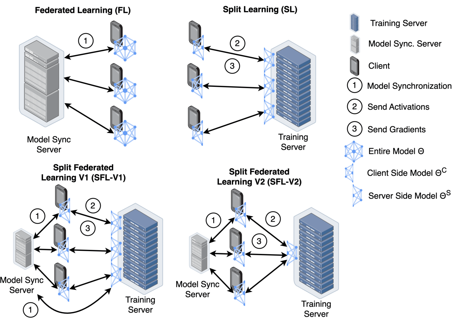
To simulate Split Federated Learning (SFL), we do not employ the approach of physically splitting the model in code implementation. Instead, we independently maintain different parts of the model's parameters. We simulate Client training in a serial manner, without actual Client parallelism.
Split Learning Split learning is a method of distributed deep learning training, where a machine learning model is split into multiple parts and trained across multiple machines or devices without needing to share the full data or model. This ensures the security and privacy of data, particularly in applications requiring privacy protection such as healthcare, finance, or when devices lack the computational resources to train the full model. How Split Learning Works: Model splitting : The deep learning model is divided into two (or more) parts. For example, part of the model may run on the user device (edge device), while the controller function run on the server. Communication process : The user device trains a portion of the model based on its local data or data from another device and sends the intermediate activations to the next layer's machine instead of sending the full data. The clients at the last layers will calculate the backward pass and return the corresponding gradients to the user device to update the part of the model. This process repeats until the model completes training. After completing a training round, the server receives the parameters from the clients and continues distributing the new model to the necessary clients for the next round. Advantages of Split Learning: Privacy protection : Sensitive data does not need to be fully transferred between devices and servers. Instead, only the intermediate activations are shared. Resource-saving : Devices with limited computational resources (such as mobile phones) can share the load and jointly train a smaller portion of the model compared to the original DNN. Model scalability : Split learning allows the model to be split across multiple devices, extending the capability to handle larger models. Deployment Model To deploy the service, each blocks in the system (server and clients) need to ensure the following requirements: All must be successfully connected to the same queue server, which serves as the main communication hub for the entire system. The server must be correctly configured with the topology and the DNN model loaded. The clients must synchronize with each other when the model is split and joined according to the topology agreed upon with the server. Clients training flow: Required Packages torch torchvision pika tqdm pyyaml Set up a RabbitMQ server for message communication over the network environment. docker-compose.yaml file: version : ' 3 ' services : rabbitmq : image : rabbitmq:management container_name : rabbitmq ports : - " 5672:5672 " # RabbitMQ main port - " 15672:15672 " # Management UI environment : RABBITMQ_DEFAULT_USER : user RABBITMQ_DEFAULT_PASS : password volumes : - rabbitmq_data:/var/lib/rabbitmq volumes : rabbitmq_data : driver : local Then run the RabbitMQ container docker-compose up -d Configuration Application configuration is in the config.yaml file: name : Split Learning server : # server configuration local-round : 1 global-round : 1 clients : # all devices in system - 2 - 2 # layer 1 has 2 devices, layer 2 has 2 devices no-cluster : cut-layers : [7] # general cut-point cluster : num-cluster : 1 # number of cluster cut-layers : - [7] # cut-point in cluster 0 - [14] # cut-point in cluster 1 infor-cluster : - [1,1] # cluster 0 has 1 device in layer 1 and 1 client in layer 2 - [1,1] # cluster 1 has 1 device in layer 1 and 1 client in layer 2 model : VGG16 # model name data-name : CIFAR10 # training data: MNIST, CIFAR10 parameters : load : False # allow to load parameters file save : False # allow to save parameters file # if turn on, server will be averaging all parameters validation : False # allow to validate on server-side data-distribution : # data distribution config num-label : 10 # number of label in dataset num-data-range : # minimum and maximum number of label's data - 250 - 250 non-iid-rate : 1 # non-IID rate, range (0, 1] refresh-each-round : True # if set True, non-IID on label will be reset on each round random-seed : 1 client-cluster : # mode cluster configuration enable : False # run cluster auto-partition : False # use algorithm cluster syn-cut-layers : False special : False # use mode only aggregate layer 1 cluster : AffinityPropagation # choose cluster algorithm AffinityPropagation : # cluster algorithm configuration damping : 0.9 max_iter : 1000 rabbit : # RabbitMQ connection configuration address : 127.0.0.1 username : admin password : admin virtual-host : \ log_path : . debug_mode : True learning : learning-rate : 0.01 momentum : 0.5 batch-size : 32 control-count : 3 This configuration is use for server. List of DNN model For server.model field: VGG16 How to Run Alter your configuration, you need to run the server to listen and control the request from clients. Server python server.py Client Now, when server is ready, run clients simultaneously with total number of client that you defined. Layer 1 python client.py --layer_id 1 --performance 0 Where: --layer_id is the ID index of client's layer, start from 1. --performance is the performance of device If you want to use a specific device configuration for the training process, declare it with the --device argument when running the command line: python client.py --layer_id 1 --performance 0 --device cpu Parameter Files On the server, the *.pth files are saved in the main execution directory of server.py after completing one training round. If the *.pth file exists, the server will read the file and send the parameters to the clients. Otherwise, if the file does not exist, a new DNN model will be created with fresh parameters. Therefore, if you want to reset the training process, you should delete the *.pth files. Version 3.0.0 The application is under development... TODO: Inference mode and training mode Delete all queues alter finish Create close connection request
Split learning is a method of distributed deep learning training, where a machine learning model is split into multiple parts and trained across multiple machines or devices without needing to share the full data or model. This ensures the security and privacy of data, particularly in applications requiring privacy protection such as healthcare, finance, or when devices lack the computational resources to train the full model.
To deploy the service, each blocks in the system (server and clients) need to ensure the following requirements:
Set up a RabbitMQ server for message communication over the network environment. docker-compose.yaml file:
version : ' 3 ' services : rabbitmq : image : rabbitmq:management container_name : rabbitmq ports : - " 5672:5672 " # RabbitMQ main port - " 15672:15672 " # Management UI environment : RABBITMQ_DEFAULT_USER : user RABBITMQ_DEFAULT_PASS : password volumes : - rabbitmq_data:/var/lib/rabbitmq volumes : rabbitmq_data : driver : local
Model Figures & Evaluation Curves (4 Images)
Deep Learning Execution Pipeline
(Preprocessing)
(Feature Extraction)
(Self-Attention)
(Loss Optimization)