Squeezenet Lightweight Ai | AI Final Year Project Report

Complete Technical Paper Content — Squeezenet Lightweight Ai

1. Executive Abstract, Problem Formulation & Background

In our previous post , we took a deep dive into the theory behind the landmark SqueezeNet paper. We deconstructed the “why”—the motivations and the brilliant design strategies that allowed researchers to achieve AlexNet-level performance with a model over 500 times smaller.

Reading a paper is one thing, but true understanding often comes from implementation. The goal of this post is to translate the concepts from the SqueezeNet paper into a complete, working PyTorch model. We’ll walk through the code step-by-step, build the architecture from the ground up, train it on a real dataset, and analyze the results to see if we can replicate the incredible efficiency that made SqueezeNet famous.

The complete Jupyter Notebook for this post is available on GitHub. You can view it, download it, and run the code yourself at the following link:

I ran this notebook on an AWS SageMaker Notebook Instance with the instance type ml.g4dn.xlarge and platform identifier Amazon Linux 2, JupyterLab 4 . The g4dn.xlarge instance belongs to the GPU family and comes with 4 vCPUs, 16 GiB of memory, and 1 NVIDIA T4 Tensor Core GPU .

Alternatively, you can use Google Colab , which provides free access to the same type of GPU and is an excellent platform for running Jupyter notebooks. I tested the notebook on Colab with the free-tier T4 GPU, and it worked seamlessly. The training loop takes around 1.5 hours to complete on Colab.

In my experience, training completes faster on the g4dn.xlarge instance compared to Colab.

The original SqueezeNet was trained on the massive ImageNet dataset, which contains over a million images across 1000 categories. Training on ImageNet from scratch requires immense computational resources and time.

For this post, we’ll use the popular CIFAR-10 dataset. It consists of 60,000 32x32 color images in 10 classes, such as ‘plane’, ‘car’, ‘bird’, and ‘dog’. CIFAR-10 is a fantastic learning tool because it’s complex enough to be a meaningful challenge, but small enough that we can train our network in a reasonable amount of time on a single GPU. It’s the perfect environment to validate our SqueezeNet implementation.

We will follow the logical flow of a machine learning project, from data preparation to final analysis. Here’s what we’ll cover:

Before we can build our network, we need to prepare our data. A robust and efficient data pipeline is the foundation of any successful deep learning project. In this section, we’ll handle three key steps: setting up our environment, defining our data transformations (including augmentation), and creating optimized data loaders to feed the GPU.

First, we’ll import all the necessary libraries. We’re using PyTorch for building and training the model, Matplotlib for plotting, and a few other helpful utilities. For reproducibility, it’s great practice to log the versions of our key libraries using watermark . This helps ensure that others (or our future selves!) can recreate the same environment.

import torch import torchvision import torchvision.transforms as transforms import torch.nn as nn import torch.optim as optim import torch.nn.init as init import os import matplotlib.pyplot as plt import numpy as np from torch.optim.lr_scheduler import ReduceLROnPlateau from tqdm import tqdm % matplotlib inline

Python implementation: CPython Python version : 3.10.18 IPython version : 8.37.0 torch : 2.6.0+cu124 torchvision: 0.21.0+cu124 matplotlib : 3.10.5 watermark : 2.5.0 tqdm : 4.67.1 Compiler : GCC 13.3.0 OS : Linux Release : 5.10.240-238.959.amzn2.x86_64 Machine : x86_64 Processor : x86_64 CPU cores : 4 Architecture: 64bit

Raw image data is rarely fed directly into a neural network. We need to process it first. We’ll define two separate transformation pipelines: one for our training data and one for our validation/testing data.

Our train_transform is a sequence of operations designed to prepare the data and also to augment it. Data augmentation is a powerful technique to artificially increase the diversity of your training set and prevent the model from overfitting.

# For training: resize, augment, convert to tensor, normalize train_transform = transforms.Compose([ transforms.Resize( 224 ), transforms.RandomHorizontalFlip(), transforms.RandomRotation( 10 ), transforms.ToTensor(), transforms.Normalize(( 0.5 , 0.5 , 0.5 ), ( 0.5 , 0.5 , 0.5 )) ])

Our test_transform is simpler. We perform the necessary resizing, conversion to a tensor, and normalization, but we do not use augmentation. We want to evaluate our model on the clean, original test data, not modified versions of it.

# For validation/testing: just resize, convert to tensor, normalize test_transform = transforms.Compose([ transforms.Resize( 224 ), transforms.ToTensor(), transforms.Normalize(( 0.5 , 0.5 , 0.5 ), ( 0.5 , 0.5 , 0.5 )) ])

Now that we have our transformation pipelines, we’ll create PyTorch DataLoaders . A DataLoader is a powerful utility that automatically handles batching our data, shuffling it, and loading it in parallel.

We’ll pay attention to a few key parameters to make our data pipeline as fast as possible:

# --- Data Loading and Augmentation --- # For training: resize, augment, convert to tensor, normalize train_transform = transforms.Compose([ transforms.Resize( 224 ), transforms.RandomHorizontalFlip(), transforms.RandomRotation( 10 ), transforms.ToTensor(), transforms.Normalize(( 0.5 , 0.5 , 0.5 ), ( 0.5 , 0.5 , 0.5 )) ]) # For validation/testing: just resize, convert to tensor, normalize test_transform = transforms.Compose([ transforms.Resize( 224 ), transforms.ToTensor(), transforms.Normalize(( 0.5 , 0.5 , 0.5 ), ( 0.5 , 0.5 , 0.5 )) ]) # --- Data Loader Optimizations --- # Increased batch size for better GPU utilization batch_size = 128 # Use more workers to load data in parallel # Use os.cpu_count() for a good starting point, but you may need to tune this num_workers = min (os.cpu_count(), 8 ) print ( "num_workers: " , num_workers) trainset = torchvision.datasets.CIFAR10(root = './data' , train = True , download = True , transform = train_transform) # Enabled pin_memory=True for faster CPU to GPU data transfer trainloader = torch.utils.data.DataLoader(trainset, batch_size = batch_size, shuffle = True , num_workers = num_workers, pin_memory = True ) testset = torchvision.datasets.CIFAR10(root = './data' , train = False , download = True , transform = test_transform) testloader = torch.utils.data.DataLoader(testset, batch_size = batch_size, shuffle = False , num_workers = num_workers, pin_memory = True ) classes = ( 'plane' , 'car' , 'bird' , 'cat' , 'deer' , 'dog' , 'frog' , 'horse' , 'ship' , 'truck' )

Before we move on to building our model, it’s always a good idea to perform a quick sanity check to make sure our data pipeline is working as expected. Let’s grab one batch of images from our trainloader and display them with their correct labels.

# --- Get a batch of training data --- # Create an iterator from the dataloader dataiter = iter (trainloader) # Get the first batch of images and labels images, labels = next (dataiter) # --- Define a function to display an image --- # This function will un-normalize and display a single image tensor def imshow(img): img = img / 2 + 0.5 # Un-normalize the image npimg = img.numpy() plt.imshow(np.transpose(npimg, ( 1 , 2 , 0 ))) # Convert from Tensor image # --- Create a grid of images and display them --- # Number of images to display num_images_to_show = 10 # Create a figure with a grid of subplots # We'll use 2 rows and 5 columns to display 10 images fig, axes = plt.subplots(nrows = 2 , ncols = 5 , figsize = ( 15 , 6 )) # Flatten the axes array to make it easy to loop over axes = axes.flatten() for i in range (num_images_to_show): ax = axes[i] # Detach the image tensor, move to CPU, and un-normalize img = images[i].cpu() img = img / 2 + 0.5 # Un-normalize npimg = img.numpy() # Display the image ax.imshow(np.transpose(npimg, ( 1 , 2 , 0 ))) # Set the title of the subplot to the corresponding class label ax.set_title(classes[labels[i]]) # Remove the x and y axis ticks for a cleaner look ax.set_xticks([]) ax.set_yticks([]) # Add a title for the entire figure and adjust layout plt.suptitle( 'Sample Training Images with Labels' , fontsize = 16 ) plt.tight_layout(rect = [ 0 , 0 , 1 , 0.96 ]) # Adjust layout to make room for suptitle plt.show()

With our data pipeline ready, it’s time to build the engine of SqueezeNet: the Fire module. As we learned in our theory deep-dive, this compact and efficient module is the key to SqueezeNet’s small size and high performance.

2. Related Work, Literature Survey & Algorithmic Foundations

We’ll implement the Fire module as a custom class that inherits from PyTorch’s nn.Module . This allows us to define its constituent layers in the __init__ method and specify how data flows through them in the forward method.

class Fire(nn.Module): def __init__ ( self , inplanes: int , squeeze_planes: int , expand1x1_planes: int , expand3x3_planes: int ) -> None : super (). __init__ () self .inplanes = inplanes # Squeeze Layer self .squeeze = nn.Conv2d(inplanes, squeeze_planes, kernel_size = 1 ) self .squeeze_activation = nn.ReLU(inplace = True ) # Expand Layer - 1x1 branch self .expand1x1 = nn.Conv2d(squeeze_planes, expand1x1_planes, kernel_size = 1 ) self .expand1x1_activation = nn.ReLU(inplace = True ) # Expand Layer - 3x3 branch self .expand3x3 = nn.Conv2d(squeeze_planes, expand3x3_planes, kernel_size = 3 , padding = 1 ) self .expand3x3_activation = nn.ReLU(inplace = True ) def forward( self , x: torch.Tensor) -> torch.Tensor: # Squeeze the input x = self .squeeze_activation( self .squeeze(x)) # Pass through both expand branches and concatenate the results return torch.cat( [ self .expand1x1_activation( self .expand1x1(x)), self .expand3x3_activation( self .expand3x3(x))], 1 )

This clean and modular implementation gives us the reusable building block we need to construct the full SqueezeNet architecture.

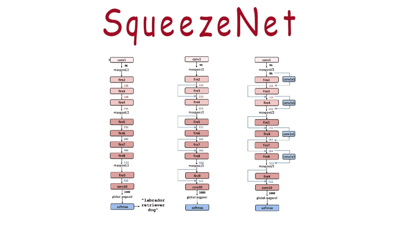
Now that we have our Fire module “LEGO brick,” we can stack them together to build the complete SqueezeNet macroarchitecture, just as described in Table 1 of the paper .

class SqueezeNet(nn.Module): def __init__ ( self , num_classes: int = 10 , dropout: float = 0.5 ) -> None : super (). __init__ () self .num_classes = num_classes # Feature extractor, following the paper's architecture self .features = nn.Sequential( nn.Conv2d( 3 , 96 , kernel_size = 7 , stride = 2 ), nn.ReLU(inplace = True ), nn.MaxPool2d(kernel_size = 3 , stride = 2 , ceil_mode = True ), Fire( 96 , 16 , 64 , 64 ), Fire( 128 , 16 , 64 , 64 ), Fire( 128 , 32 , 128 , 128 ), nn.MaxPool2d(kernel_size = 3 , stride = 2 , ceil_mode = True ), Fire( 256 , 32 , 128 , 128 ), Fire( 256 , 48 , 192 , 192 ), Fire( 384 , 48 , 192 , 192 ), Fire( 384 , 64 , 256 , 256 ), nn.MaxPool2d(kernel_size = 3 , stride = 2 , ceil_mode = True ), Fire( 512 , 64 , 256 , 256 ), ) # Final convolution is initialized differently from the rest final_conv = nn.Conv2d( 512 , self .num_classes, kernel_size = 1 ) # Classifier head self .classifier = nn.Sequential( nn.Dropout(p = dropout), final_conv, nn.ReLU(inplace = True ), nn.AdaptiveAvgPool2d(( 1 , 1 )) ) for m in self .modules(): if isinstance (m, nn.Conv2d): if m is final_conv: init.normal_(m.weight, mean = 0.0 , std = 0.01 ) else : init.kaiming_uniform_(m.weight) if m.bias is not None : init.constant_(m.bias, 0 ) def forward( self , x: torch.Tensor) -> torch.Tensor: x = self .features(x) x = self .classifier(x) return torch.flatten(x, 1 )

With just these two classes, we have a complete implementation of the entire SqueezeNet architecture. Now, let’s train it!

We have our data pipeline and our model architecture. Now, let’s put them together and train our SqueezeNet model on the CIFAR-10 dataset. We’ll set up a robust training loop and then analyze the output to understand how our model learned over time.

# --- Model, Optimizer, and Training Setup --- device = torch.device( 'cuda:0' if torch.cuda.is_available() else 'cpu' ) print ( f"Using device: { device } " ) net = SqueezeNet() # initialize your model net.to(device) # --- Compile the model (PyTorch 2.0+ feature) --- # This is a massive speedup! if torch.__version__[ 0 ] == '2' : print ( "PyTorch 2.0+ detected. Compiling the model..." ) net = torch. compile (net)

criterion = nn.CrossEntropyLoss() # Using a potentially faster-converging optimizer optimizer = optim.AdamW(net.parameters(), lr = 0.001 , weight_decay = 1e-4 ) num_epochs = 40

# --- DEFINE THE ReduceLROnPlateau SCHEDULER --- # This scheduler monitors the validation loss. # 'patience=2': Wait for 2 epochs of no improvement before reducing LR. # 'factor=0.1': Reduce LR by a factor of 10 (e.g., 0.001 -> 0.0001). # 'mode=min': It's monitoring a value that should be minimized (loss). scheduler = ReduceLROnPlateau(optimizer, mode = 'min' , factor = 0.1 , patience = 2 )

# --- EARLY STOPPING SETUP --- # Path to save the best model SAVE_PATH = 'best_model.pth' # Initialize variables to track the best performance best_val_loss = float ( 'inf' ) best_epoch = 0

# --- History Tracking --- history = { 'train_loss' : [], 'val_loss' : [], 'train_acc' : [], 'val_acc' : [], 'learning_rate' : [] # Let's also track the learning rate to plot it! }

Our training loop runs for a total of 40 epochs. In each epoch, it performs a full pass over the training data to update the model’s weights, followed by a full pass over the validation data to check its performance on unseen images.

print ( "Starting Training..." ) for epoch in range (num_epochs): # --- Training Phase --- net.train() train_loss = 0.0 correct_train = 0 total_train = 0 current_lr = optimizer.param_groups[ 0 ][ 'lr' ] train_bar = tqdm(trainloader, desc = f"Epoch { epoch + 1 } / { num_epochs } [Training] LR: { current_lr :.6f} " ) for data in train_bar: inputs, labels = data[ 0 ].to(device, non_blocking = True ), data[ 1 ].to(device, non_blocking = True ) optimizer.zero_grad(set_to_none = True ) outputs = net(inputs) loss = criterion(outputs, labels) loss.backward() optimizer.step() train_loss += loss.item() _, predicted = torch. max (outputs.data, 1 ) total_train += labels.size( 0 ) correct_train += (predicted == labels). sum ().item() train_bar.set_postfix(loss = loss.item()) avg_train_loss = train_loss / len (trainloader) train_accuracy = 100 * correct_train / total_train history[ 'train_loss' ].append(avg_train_loss) history[ 'train_acc' ].append(train_accuracy) history[ 'learning_rate' ].append(current_lr) # --- Validation Phase --- net. eval () val_loss = 0.0 correct_val = 0 total_val = 0 val_bar = tqdm(testloader, desc = f"Epoch { epoch + 1 } / { num_epochs } [Validation]" ) with torch.no_grad(): for data in val_bar: inputs, labels = data[ 0 ].to(device, non_blocking = True ), data[ 1 ].to(device, non_blocking = True ) outputs = net(inputs) loss = criterion(outputs, labels) val_loss += loss.item() _, predicted = torch. max (outputs.data, 1 ) total_val += labels.size( 0 ) correct_val += (predicted == labels). sum ().item() val_bar.set_postfix(loss = loss.item()) avg_val_loss = val_loss / len (testloader) val_accuracy = 100 * correct_val / total_val history[ 'val_loss' ].append(avg_val_loss) history[ 'val_acc' ].append(val_accuracy) # --- EARLY STOPPING LOGIC --- # Check if the current validation loss is the best we've seen so far. if avg_val_loss < best_val_loss: best_val_loss = avg_val_loss best_epoch = epoch + 1 # Save the model's state dictionary torch.save(net._orig_mod.state_dict(), SAVE_PATH) print ( f" \n ---> New best model saved at epoch { best_epoch } with validation loss: { best_val_loss :.4f} \n " ) scheduler.step(avg_val_loss) print ( f" \n Epoch { epoch + 1 } / { num_epochs } Summary:" ) print ( f" Train Loss: { avg_train_loss :.4f} | Train Acc: { train_accuracy :.2f} %" ) print ( f" Valid Loss: { avg_val_loss :.4f} | Valid Acc: { val_accuracy :.2f} %" ) print ( f" Current LR: { optimizer . param_groups[ 0 ][ 'lr' ] :.6f} \n " ) print ( 'Finished Training' ) print ( f"The best model was saved from epoch { best_epoch } at path: { SAVE_PATH } " )

Epoch 1/40 [Training] LR: 0.001000: 100%|██████████| 391/391 [01:47<00:00, 3.64it/s, loss=1.93] Epoch 1/40 [Validation]: 100%|██████████| 79/79 [00:10<00:00, 7.34it/s, loss=1.75]

---> New best model saved at epoch 1 with validation loss: 1.8390 Epoch 1/40 Summary: Train Loss: 2.0931 | Train Acc: 21.73% Valid Loss: 1.8390 | Valid Acc: 31.86% Current LR: 0.001000

Epoch 2/40 [Training] LR: 0.001000: 100%|██████████| 391/391 [01:39<00:00, 3.94it/s, loss=1.6] Epoch 2/40 [Validation]: 100%|██████████| 79/79 [00:08<00:00, 8.80it/s, loss=1.72]

---> New best model saved at epoch 2 with validation loss: 1.6319 Epoch 2/40 Summary: Train Loss: 1.7570 | Train Acc: 36.83% Valid Loss: 1.6319 | Valid Acc: 41.62% Current LR: 0.001000

Epoch 3/40 [Training] LR: 0.001000: 100%|██████████| 391/391 [01:39<00:00, 3.93it/s, loss=1.65] Epoch 3/40 [Validation]: 100%|██████████| 79/79 [00:09<00:00, 8.70it/s, loss=1.76]

---> New best model saved at epoch 3 with validation loss: 1.5504 Epoch 3/40 Summary: Train Loss: 1.5792 | Train Acc: 45.08% Valid Loss: 1.5504 | Valid Acc: 46.14% Current LR: 0.001000

Epoch 4/40 [Training] LR: 0.001000: 100%|██████████| 391/391 [01:39<00:00, 3.93it/s, loss=1.31] Epoch 4/40 [Validation]: 100%|██████████| 79/79 [00:08<00:00, 8.81it/s, loss=1.59]

---> New best model saved at epoch 4 with validation loss: 1.1688 Epoch 4/40 Summary: Train Loss: 1.3565 | Train Acc: 52.19% Valid Loss: 1.1688 | Valid Acc: 58.67% Current LR: 0.001000

Epoch 5/40 [Training] LR: 0.001000: 100%|██████████| 391/391 [01:39<00:00, 3.92it/s, loss=1.18] Epoch 5/40 [Validation]: 100%|██████████| 79/79 [00:08<00:00, 8.78it/s, loss=1.56]

---> New best model saved at epoch 5 with validation loss: 1.1274 Epoch 5/40 Summary: Train Loss: 1.1526 | Train Acc: 58.94% Valid Loss: 1.1274 | Valid Acc: 61.63% Current LR: 0.001000

3. Dataset Ingestion, Preprocessing & Stochastic Augmentations

Epoch 6/40 [Training] LR: 0.001000: 100%|██████████| 391/391 [01:39<00:00, 3.92it/s, loss=1.02] Epoch 6/40 [Validation]: 100%|██████████| 79/79 [00:08<00:00, 8.79it/s, loss=1.23]

---> New best model saved at epoch 6 with validation loss: 0.9898 Epoch 6/40 Summary: Train Loss: 1.0576 | Train Acc: 62.63% Valid Loss: 0.9898 | Valid Acc: 65.36% Current LR: 0.001000

Epoch 7/40 [Training] LR: 0.001000: 100%|██████████| 391/391 [01:39<00:00, 3.93it/s, loss=1.11] Epoch 7/40 [Validation]: 100%|██████████| 79/79 [00:09<00:00, 8.71it/s, loss=1.07]

---> New best model saved at epoch 7 with validation loss: 0.9031 Epoch 7/40 Summary: Train Loss: 0.9776 | Train Acc: 65.39% Valid Loss: 0.9031 | Valid Acc: 68.49% Current LR: 0.001000

Epoch 8/40 [Training] LR: 0.001000: 100%|██████████| 391/391 [01:39<00:00, 3.93it/s, loss=0.938] Epoch 8/40 [Validation]: 100%|██████████| 79/79 [00:09<00:00, 8.74it/s, loss=1.17]

---> New best model saved at epoch 8 with validation loss: 0.8737 Epoch 8/40 Summary: Train Loss: 0.9200 | Train Acc: 67.50% Valid Loss: 0.8737 | Valid Acc: 69.74% Current LR: 0.001000

Epoch 9/40 [Training] LR: 0.001000: 100%|██████████| 391/391 [01:39<00:00, 3.93it/s, loss=1.02] Epoch 9/40 [Validation]: 100%|██████████| 79/79 [00:09<00:00, 8.65it/s, loss=1.17]

---> New best model saved at epoch 9 with validation loss: 0.8723 Epoch 9/40 Summary: Train Loss: 0.8787 | Train Acc: 69.02% Valid Loss: 0.8723 | Valid Acc: 69.43% Current LR: 0.001000

Epoch 10/40 [Training] LR: 0.001000: 100%|██████████| 391/391 [01:39<00:00, 3.92it/s, loss=0.826] Epoch 10/40 [Validation]: 100%|██████████| 79/79 [00:09<00:00, 8.60it/s, loss=1.01]

Epoch 10/40 Summary: Train Loss: 0.8413 | Train Acc: 70.54% Valid Loss: 0.9084 | Valid Acc: 68.65% Current LR: 0.001000

Epoch 11/40 [Training] LR: 0.001000: 100%|██████████| 391/391 [01:39<00:00, 3.92it/s, loss=0.689] Epoch 11/40 [Validation]: 100%|██████████| 79/79 [00:09<00:00, 8.58it/s, loss=0.941]

---> New best model saved at epoch 11 with validation loss: 0.8162 Epoch 11/40 Summary: Train Loss: 0.8002 | Train Acc: 71.84% Valid Loss: 0.8162 | Valid Acc: 71.49% Current LR: 0.001000

Epoch 12/40 [Training] LR: 0.001000: 100%|██████████| 391/391 [01:39<00:00, 3.93it/s, loss=0.683] Epoch 12/40 [Validation]: 100%|██████████| 79/79 [00:09<00:00, 8.68it/s, loss=1.09]

---> New best model saved at epoch 12 with validation loss: 0.7833 Epoch 12/40 Summary: Train Loss: 0.7779 | Train Acc: 72.71% Valid Loss: 0.7833 | Valid Acc: 72.92% Current LR: 0.001000

Epoch 13/40 [Training] LR: 0.001000: 100%|██████████| 391/391 [01:39<00:00, 3.92it/s, loss=0.838] Epoch 13/40 [Validation]: 100%|██████████| 79/79 [00:09<00:00, 8.73it/s, loss=0.779]

Epoch 13/40 Summary: Train Loss: 0.7426 | Train Acc: 73.95% Valid Loss: 0.7906 | Valid Acc: 73.53% Current LR: 0.001000

Epoch 14/40 [Training] LR: 0.001000: 100%|██████████| 391/391 [01:39<00:00, 3.93it/s, loss=0.911] Epoch 14/40 [Validation]: 100%|██████████| 79/79 [00:09<00:00, 8.64it/s, loss=0.651]

---> New best model saved at epoch 14 with validation loss: 0.7424 Epoch 14/40 Summary: Train Loss: 0.7237 | Train Acc: 74.84% Valid Loss: 0.7424 | Valid Acc: 74.53% Current LR: 0.001000

Epoch 15/40 [Training] LR: 0.001000: 100%|██████████| 391/391 [01:39<00:00, 3.93it/s, loss=0.681] Epoch 15/40 [Validation]: 100%|██████████| 79/79 [00:09<00:00, 8.68it/s, loss=0.989]

---> New best model saved at epoch 15 with validation loss: 0.6920 Epoch 15/40 Summary: Train Loss: 0.7021 | Train Acc: 75.52% Valid Loss: 0.6920 | Valid Acc: 76.06% Current LR: 0.001000

Epoch 16/40 [Training] LR: 0.001000: 100%|██████████| 391/391 [01:39<00:00, 3.93it/s, loss=0.608] Epoch 16/40 [Validation]: 100%|██████████| 79/79 [00:09<00:00, 8.68it/s, loss=0.713]

---> New best model saved at epoch 16 with validation loss: 0.6897 Epoch 16/40 Summary: Train Loss: 0.6817 | Train Acc: 76.48% Valid Loss: 0.6897 | Valid Acc: 76.15% Current LR: 0.001000

Epoch 17/40 [Training] LR: 0.001000: 100%|██████████| 391/391 [01:39<00:00, 3.94it/s, loss=0.516] Epoch 17/40 [Validation]: 100%|██████████| 79/79 [00:09<00:00, 8.66it/s, loss=0.491]

---> New best model saved at epoch 17 with validation loss: 0.6855 Epoch 17/40 Summary: Train Loss: 0.6645 | Train Acc: 76.98% Valid Loss: 0.6855 | Valid Acc: 76.53% Current LR: 0.001000

4. Neural Network Backbone, Layer Specifications & Loss Formulations

Epoch 18/40 [Training] LR: 0.001000: 100%|██████████| 391/391 [01:39<00:00, 3.93it/s, loss=0.684] Epoch 18/40 [Validation]: 100%|██████████| 79/79 [00:09<00:00, 8.63it/s, loss=0.584]

Epoch 18/40 Summary: Train Loss: 0.6430 | Train Acc: 77.51% Valid Loss: 0.6882 | Valid Acc: 76.71% Current LR: 0.001000

Epoch 19/40 [Training] LR: 0.001000: 100%|██████████| 391/391 [01:39<00:00, 3.94it/s, loss=0.686] Epoch 19/40 [Validation]: 100%|██████████| 79/79 [00:09<00:00, 8.51it/s, loss=0.602]

---> New best model saved at epoch 19 with validation loss: 0.6528 Epoch 19/40 Summary: Train Loss: 0.6260 | Train Acc: 78.59% Valid Loss: 0.6528 | Valid Acc: 77.44% Current LR: 0.001000

Epoch 20/40 [Training] LR: 0.001000: 100%|██████████| 391/391 [01:39<00:00, 3.93it/s, loss=0.597] Epoch 20/40 [Validation]: 100%|██████████| 79/79 [00:09<00:00, 8.63it/s, loss=0.985]

Epoch 20/40 Summary: Train Loss: 0.6112 | Train Acc: 78.84% Valid Loss: 0.6556 | Valid Acc: 78.34% Current LR: 0.001000

Epoch 21/40 [Training] LR: 0.001000: 100%|██████████| 391/391 [01:39<00:00, 3.93it/s, loss=0.619] Epoch 21/40 [Validation]: 100%|██████████| 79/79 [00:09<00:00, 8.66it/s, loss=0.469]

---> New best model saved at epoch 21 with validation loss: 0.6311 Epoch 21/40 Summary: Train Loss: 0.6036 | Train Acc: 79.25% Valid Loss: 0.6311 | Valid Acc: 77.80% Current LR: 0.001000

Epoch 22/40 [Training] LR: 0.001000: 100%|██████████| 391/391 [01:39<00:00, 3.93it/s, loss=0.489] Epoch 22/40 [Validation]: 100%|██████████| 79/79 [00:09<00:00, 8.60it/s, loss=0.933]

---> New best model saved at epoch 22 with validation loss: 0.6292 Epoch 22/40 Summary: Train Loss: 0.5879 | Train Acc: 79.67% Valid Loss: 0.6292 | Valid Acc: 78.66% Current LR: 0.001000

Epoch 23/40 [Training] LR: 0.001000: 100%|██████████| 391/391 [01:39<00:00, 3.93it/s, loss=0.591] Epoch 23/40 [Validation]: 100%|██████████| 79/79 [00:09<00:00, 8.60it/s, loss=0.809]

Epoch 23/40 Summary: Train Loss: 0.5719 | Train Acc: 80.13% Valid Loss: 0.6631 | Valid Acc: 78.27% Current LR: 0.001000

Epoch 24/40 [Training] LR: 0.001000: 100%|██████████| 391/391 [01:39<00:00, 3.93it/s, loss=0.582] Epoch 24/40 [Validation]: 100%|██████████| 79/79 [00:09<00:00, 8.59it/s, loss=0.523]

Epoch 24/40 Summary: Train Loss: 0.5611 | Train Acc: 80.51% Valid Loss: 0.6358 | Valid Acc: 78.58% Current LR: 0.001000

Epoch 25/40 [Training] LR: 0.001000: 100%|██████████| 391/391 [01:39<00:00, 3.93it/s, loss=0.651] Epoch 25/40 [Validation]: 100%|██████████| 79/79 [00:09<00:00, 8.69it/s, loss=0.522]

---> New best model saved at epoch 25 with validation loss: 0.6080 Epoch 25/40 Summary: Train Loss: 0.5564 | Train Acc: 80.69% Valid Loss: 0.6080 | Valid Acc: 79.01% Current LR: 0.001000

Epoch 26/40 [Training] LR: 0.001000: 100%|██████████| 391/391 [01:39<00:00, 3.93it/s, loss=0.42] Epoch 26/40 [Validation]: 100%|██████████| 79/79 [00:09<00:00, 8.62it/s, loss=0.701]

Epoch 26/40 Summary: Train Loss: 0.5376 | Train Acc: 81.27% Valid Loss: 0.6286 | Valid Acc: 79.54% Current LR: 0.001000

Epoch 27/40 [Training] LR: 0.001000: 100%|██████████| 391/391 [01:39<00:00, 3.93it/s, loss=0.586] Epoch 27/40 [Validation]: 100%|██████████| 79/79 [00:09<00:00, 8.60it/s, loss=0.558]

Epoch 27/40 Summary: Train Loss: 0.5353 | Train Acc: 81.31% Valid Loss: 0.6098 | Valid Acc: 79.64% Current LR: 0.001000

Epoch 28/40 [Training] LR: 0.001000: 100%|██████████| 391/391 [01:39<00:00, 3.93it/s, loss=0.319] Epoch 28/40 [Validation]: 100%|██████████| 79/79 [00:09<00:00, 8.44it/s, loss=0.325]

---> New best model saved at epoch 28 with validation loss: 0.5744 Epoch 28/40 Summary: Train Loss: 0.5299 | Train Acc: 81.55% Valid Loss: 0.5744 | Valid Acc: 80.60% Current LR: 0.001000

Epoch 29/40 [Training] LR: 0.001000: 100%|██████████| 391/391 [01:39<00:00, 3.94it/s, loss=0.504] Epoch 29/40 [Validation]: 100%|██████████| 79/79 [00:09<00:00, 8.65it/s, loss=0.484]

Epoch 29/40 Summary: Train Loss: 0.5223 | Train Acc: 81.90% Valid Loss: 0.5836 | Valid Acc: 80.31% Current LR: 0.001000

5. Training Protocol, Convergence Behavior & Experimental Evaluation

Epoch 30/40 [Training] LR: 0.001000: 100%|██████████| 391/391 [01:39<00:00, 3.93it/s, loss=0.315] Epoch 30/40 [Validation]: 100%|██████████| 79/79 [00:09<00:00, 8.58it/s, loss=0.412]

---> New best model saved at epoch 30 with validation loss: 0.5589 Epoch 30/40 Summary: Train Loss: 0.5080 | Train Acc: 82.46% Valid Loss: 0.5589 | Valid Acc: 80.98% Current LR: 0.001000

Epoch 31/40 [Training] LR: 0.001000: 100%|██████████| 391/391 [01:39<00:00, 3.92it/s, loss=0.469] Epoch 31/40 [Validation]: 100%|██████████| 79/79 [00:09<00:00, 8.59it/s, loss=0.582]

Epoch 31/40 Summary: Train Loss: 0.5047 | Train Acc: 82.40% Valid Loss: 0.5764 | Valid Acc: 80.59% Current LR: 0.001000

Epoch 32/40 [Training] LR: 0.001000: 100%|██████████| 391/391 [01:39<00:00, 3.92it/s, loss=0.304] Epoch 32/40 [Validation]: 100%|██████████| 79/79 [00:10<00:00, 7.80it/s, loss=0.51]

Epoch 32/40 Summary: Train Loss: 0.4902 | Train Acc: 83.11% Valid Loss: 0.5664 | Valid Acc: 81.12% Current LR: 0.001000

Epoch 33/40 [Training] LR: 0.001000: 100%|██████████| 391/391 [01:39<00:00, 3.92it/s, loss=0.494] Epoch 33/40 [Validation]: 100%|██████████| 79/79 [00:09<00:00, 8.72it/s, loss=0.756]

Epoch 33/40 Summary: Train Loss: 0.4846 | Train Acc: 83.10% Valid Loss: 0.5599 | Valid Acc: 81.43% Current LR: 0.000100

Epoch 34/40 [Training] LR: 0.000100: 100%|██████████| 391/391 [01:39<00:00, 3.93it/s, loss=0.434] Epoch 34/40 [Validation]: 100%|██████████| 79/79 [00:09<00:00, 8.73it/s, loss=0.296]

---> New best model saved at epoch 34 with validation loss: 0.4800 Epoch 34/40 Summary: Train Loss: 0.3871 | Train Acc: 86.55% Valid Loss: 0.4800 | Valid Acc: 83.42% Current LR: 0.000100

Epoch 35/40 [Training] LR: 0.000100: 100%|██████████| 391/391 [01:39<00:00, 3.93it/s, loss=0.488] Epoch 35/40 [Validation]: 100%|██████████| 79/79 [00:09<00:00, 8.58it/s, loss=0.267]

Epoch 35/40 Summary: Train Loss: 0.3628 | Train Acc: 87.45% Valid Loss: 0.4835 | Valid Acc: 83.83% Current LR: 0.000100

Epoch 36/40 [Training] LR: 0.000100: 100%|██████████| 391/391 [01:39<00:00, 3.93it/s, loss=0.363] Epoch 36/40 [Validation]: 100%|██████████| 79/79 [00:09<00:00, 8.60it/s, loss=0.309]

---> New best model saved at epoch 36 with validation loss: 0.4772 Epoch 36/40 Summary: Train Loss: 0.3519 | Train Acc: 87.70% Valid Loss: 0.4772 | Valid Acc: 84.23% Current LR: 0.000100

Epoch 37/40 [Training] LR: 0.000100: 100%|██████████| 391/391 [01:39<00:00, 3.92it/s, loss=0.473] Epoch 37/40 [Validation]: 100%|██████████| 79/79 [00:10<00:00, 7.84it/s, loss=0.342]

Epoch 37/40 Summary: Train Loss: 0.3442 | Train Acc: 87.98% Valid Loss: 0.4817 | Valid Acc: 83.88% Current LR: 0.000100

Epoch 38/40 [Training] LR: 0.000100: 100%|██████████| 391/391 [01:39<00:00, 3.92it/s, loss=0.585] Epoch 38/40 [Validation]: 100%|██████████| 79/79 [00:09<00:00, 8.63it/s, loss=0.274]

Epoch 38/40 Summary: Train Loss: 0.3441 | Train Acc: 88.03% Valid Loss: 0.4802 | Valid Acc: 84.05% Current LR: 0.000100

Epoch 39/40 [Training] LR: 0.000100: 100%|██████████| 391/391 [01:39<00:00, 3.92it/s, loss=0.342] Epoch 39/40 [Validation]: 100%|██████████| 79/79 [00:09<00:00, 8.64it/s, loss=0.271]

Epoch 39/40 Summary: Train Loss: 0.3385 | Train Acc: 88.23% Valid Loss: 0.4807 | Valid Acc: 84.42% Current LR: 0.000010

Epoch 40/40 [Training] LR: 0.000010: 100%|██████████| 391/391 [01:39<00:00, 3.93it/s, loss=0.388] Epoch 40/40 [Validation]: 100%|██████████| 79/79 [00:09<00:00, 8.45it/s, loss=0.247]

---> New best model saved at epoch 40 with validation loss: 0.4746 Epoch 40/40 Summary: Train Loss: 0.3228 | Train Acc: 88.80% Valid Loss: 0.4746 | Valid Acc: 84.46% Current LR: 0.000010 Finished Training The best model was saved from epoch 40 at path: best_model.pth

As we can see from the logs, the model steadily improves. The training loss decreases, and both training and validation accuracy increase, which is exactly what we want to see.

While logs are useful, plots give us a much more intuitive understanding of the training dynamics. Let’s visualize the loss, accuracy, and learning rate over all 40 epochs.