Complete Technical Paper Content — Stable Diffusion Projects
1. Executive Abstract, Problem Formulation & Background
Stable Diffusion is a deep learning, text-to-image model released in 2022 based on diffusion techniques. The generative AI technology is the premier product of Stability AI and is considered to be a part of the ongoing AI boom. It is primarily used to generate detailed images conditioned on text descriptions, though it can also be applied to other tasks such as inpainting, outpainting, and generating image-to-image translations guided by a text prompt. Its development involved researchers from the CompVis Group at LMU Munich and Runway with a computational donation from Stability and training data from non-profit organizations. Stable Diffusion is a latent diffusion model, a kind of deep generative artificial neural network. Its code and model weights have been released publicly, and an optimized version can run on most consumer hardware equipped with a modest GPU with as little as 2.4 GB VRAM. This marked a departure from previous proprietary text-to-image models such as DALL-E and Midjourney, which were accessible only via cloud services.
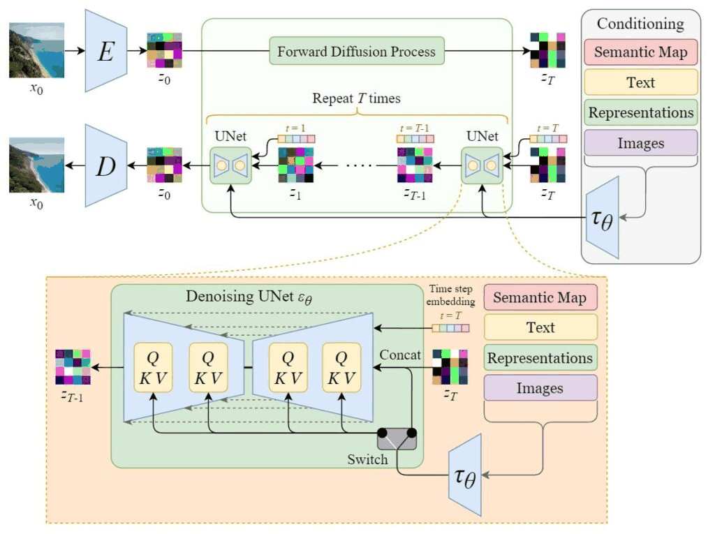
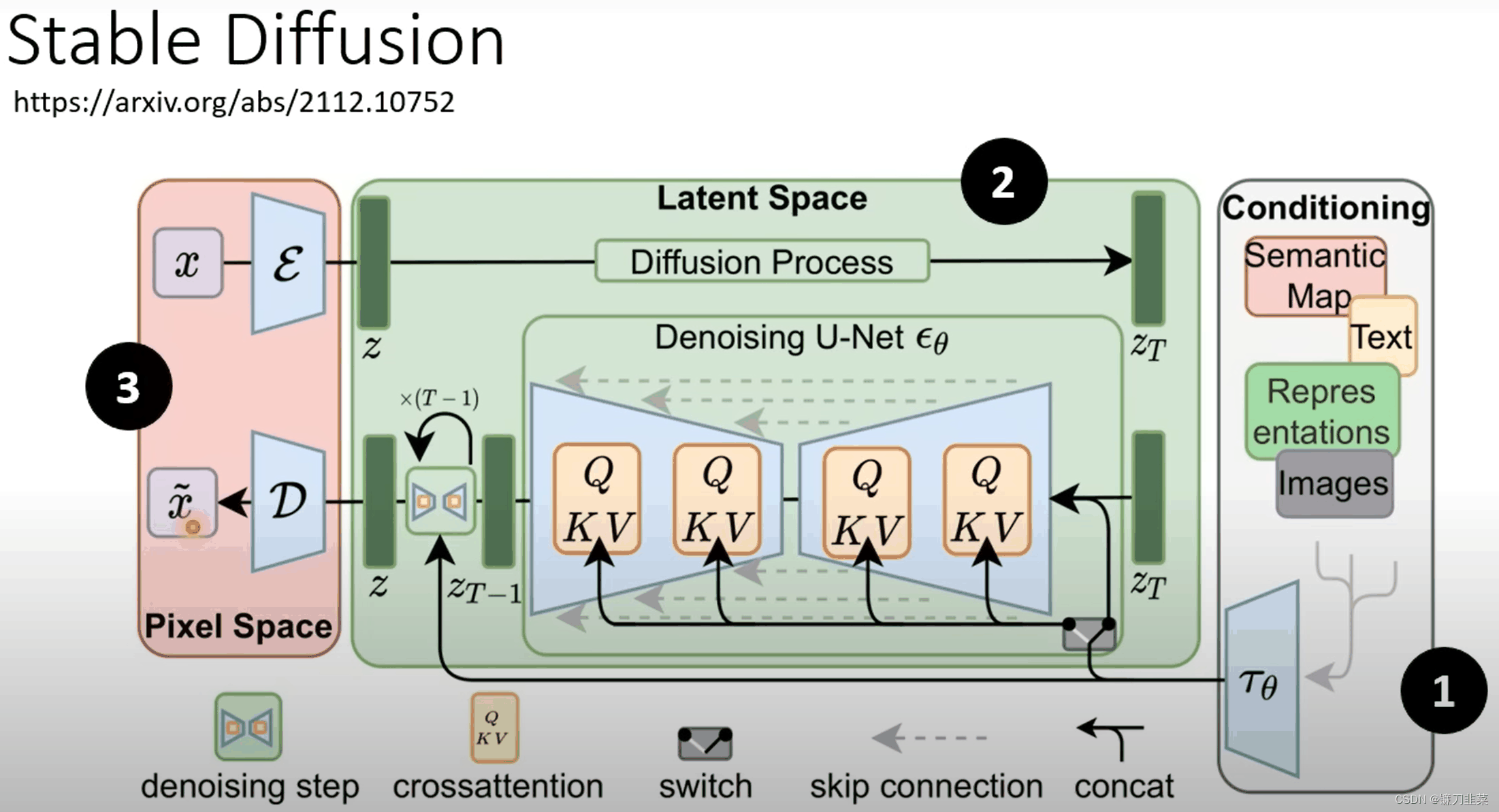
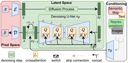
Diffusion models, introduced in 2015, are trained with the objective of removing successive applications of Gaussian noise on training images, which can be thought of as a sequence of denoising autoencoders. The name diffusion is from the thermodynamic diffusion, since they were first developed with inspiration from thermodynamics. Models in Stable Diffusion series before SD 3 all used a variant of diffusion models, called latent diffusion model (LDM), developed in 2021 by the CompVis (Computer Vision & Learning) group at LMU Munich. Stable Diffusion consists of 3 parts: the variational autoencoder (VAE), U-Net, and an optional text encoder. The VAE encoder compresses the image from pixel space to a smaller dimensional latent space, capturing a more fundamental semantic meaning of the image. Gaussian noise is iteratively applied to the compressed latent representation during forward diffusion. The U-Net block, composed of a ResNet backbone, denoises the output from forward diffusion backwards to obtain a latent representation. Finally, the VAE decoder generates the final image by converting the representation back into pixel space. The denoising step can be flexibly conditioned on a string of text, an image, or another modality. The encoded conditioning data is exposed to denoising U-Nets via a cross-attention mechanism. For conditioning on text, the fixed, pretrained CLIP ViT-L/14 text encoder is used to transform text prompts to an embedding space. Researchers point to increased computational efficiency for training and generation as an advantage of LDMs. With 860 million parameters in the U-Net and 123 million in the text encoder, Stable Diffusion is considered relatively lightweight by 2022 standards, and unlike other diffusion models, it can run on consumer GPUs, and even CPU-only if using the OpenVINO version of Stable Diffusion.
The 3.0 version completely changes the backbone. Not a UNet, but a Rectified Flow Transformer, which implements the rectified flow method with a Transformer. The Transformer architecture used for SD 3.0 has three "tracks", for original text encoding, transformed text encoding, and image encoding (in latent space). The transformed text encoding and image encoding are mixed during each transformer block. The architecture is named "multimodal diffusion transformer (MMDiT), where the "multimodal" means that it mixes text and image encodings inside its operations. This differs from previous versions of DiT, where the text encoding affects the image encoding, but not vice versa.
An "embedding" can be trained from a collection of user-provided images, and allows the model to generate visually similar images whenever the name of the embedding is used within a generation prompt. Embeddings are based on the "textual inversion" concept developed by researchers from Tel Aviv University in 2022 with support from Nvidia, where vector representations for specific tokens used by the model's text encoder are linked to new pseudo-words. Embeddings can be used to reduce biases within the original model, or mimic visual styles. A "hypernetwork" is a small pretrained neural network that is applied to various points within a larger neural network, and refers to the technique created by NovelAI developer Kurumuz in 2021, originally intended for text-generation transformer models. Hypernetworks steer results towards a particular direction, allowing Stable Diffusion-based models to imitate the art style of specific artists, even if the artist is not recognised by the original model; they process the image by finding key areas of importance such as hair and eyes, and then patch these areas in secondary latent space. DreamBooth is a deep learning generation model developed by researchers from Google Research and Boston University in 2022 which can fine-tune the model to generate precise, personalised outputs that depict a specific subject, following training via a set of images which depict the subject.
The text to image sampling script within Stable Diffusion, known as "txt2img", consumes a text prompt in addition to assorted option parameters covering sampling types, output image dimensions, and seed values. The script outputs an image file based on the model's interpretation of the prompt. Generated images are tagged with an invisible digital watermark to allow users to identify an image as generated by Stable Diffusion, although this watermark loses its efficacy if the image is resized or rotated. Each txt2img generation will involve a specific seed value which affects the output image. Users may opt to randomize the seed in order to explore different generated outputs, or use the same seed to obtain the same image output as a previously generated image. Users are also able to adjust the number of inference steps for the sampler; a higher value takes a longer duration of time, however a smaller value may result in visual defects. Another configurable option, the classifier-free guidance scale value, allows the user to adjust how closely the output image adheres to the prompt. More experimentative use cases may opt for a lower scale value, while use cases aiming for more specific outputs may use a higher value. Additional text2img features are provided by front-end implementations of Stable Diffusion, which allow users to modify the weight given to specific parts of the text prompt. Emphasis markers allow users to add or reduce emphasis to keywords by enclosing them with brackets. An alternative method of adjusting weight to parts of the prompt are "negative prompts". Negative prompts are a feature included in some front-end implementations, including Stability AI's own DreamStudio cloud service, and allow the user to specify prompts which the model should avoid during image generation. The specified prompts may be undesirable image features that would otherwise be present within image outputs due to the positive prompts provided by the user, or due to how the model was originally trained, with mangled human hands being a common example.
Stable Diffusion also includes another sampling script, "img2img", which consumes a text prompt, path to an existing image, and strength value between 0.0 and 1.0. The script outputs a new image based on the original image that also features elements provided within the text prompt. The strength value denotes the amount of noise added to the output image. A higher strength value produces more variation within the image but may produce an image that is not semantically consistent with the prompt provided. There are different methods for performing img2img. The main method is SDEdit, which first adds noise to an image, then denoises it as usual in text2img. The ability of img2img to add noise to the original image makes it potentially useful for data anonymization and data augmentation, in which the visual features of image data are changed and anonymized. The same process may also be useful for image upscaling, in which the resolution of an image is increased, with more detail potentially being added to the image. Additionally, Stable Diffusion has been experimented with as a tool for image compression. Compared to JPEG and WebP, the recent methods used for image compression in Stable Diffusion face limitations in preserving small text and faces. Additional use-cases for image modification via img2img are offered by numerous front-end implementations of the Stable Diffusion model. Inpainting involves selectively modifying a portion of an existing image delineated by a user-provided layer mask, which fills the masked space with newly generated content based on the provided prompt. A dedicated model specifically fine-tuned for inpainting use-cases was created by Stability AI alongside the release of Stable Diffusion 2.0. Conversely, outpainting extends an image beyond its original dimensions, filling the previously empty space with content generated based on the provided prompt. A depth-guided model, named "depth2img", was introduced with the release of Stable Diffusion 2.0 on November 24, 2022; this model infers the depth of the provided input image, and generates a new output image based on both the text prompt and the depth information, which allows the coherence and depth of the original input image to be maintained in the generated output.
Learning Transferable Visual Models From Natural Language Supervision (2021). This paper describes the CLIP method for training text encoders, which convert text into floating point vectors. Such text encodings are used by the diffusion model to create images. SDEdit: Guided Image Synthesis and Editing with Stochastic Differential Equations (2021). This paper describes SDEdit, aka "img2img". High-Resolution Image Synthesis with Latent Diffusion Models (2021, updated in 2022). This paper describes the latent diffusion model (LDM). This is the backbone of the Stable Diffusion architecture. Classifier-Free Diffusion Guidance (2022). This paper describes CFG, which allows the text encoding vector to steer the diffusion model towards creating the image described by the text. SDXL: Improving Latent Diffusion Models for High-Resolution Image Synthesis (2023). Describes SDXL. Flow Straight and Fast: Learning to Generate and Transfer Data with Rectified Flow (2022). Describes rectified flow, which is used for the backbone architecture of SD 3.0. Scaling Rectified Flow Transformers for High-resolution Image Synthesis (2024). Describes SD 3.0. Training cost
SD 2.0: 0.2 million hours on A100 (40GB). Stable Diffusion 3.5 Large was made available for enterprise usage on Amazon Bedrock of Amazon Web Services.
Getty Images asserted that the training and development of Stable Diffusion involved the unauthorized use of its images, which were downloaded on servers and computers that were potentially in the UK. However, Stability AI argued that all training and development took place outside the UK, specifically in U.S. data centers operated by Amazon Web Services. Stability AI applied for reverse summary judgment and/or strike out of two claims: the training and development claim, and the secondary infringement of copyright claim. The High Court, however, refused to strike out these claims, allowing them to proceed to trial. The court is to determine whether the training and development of Stable Diffusion occurred in the UK, which is crucial for establishing jurisdiction under the UK's Copyright, Designs and Patents Act 1988 (CDPA). The secondary infringement claim revolved around whether the pre-trained Stable Diffusion software, made available in the UK through platforms like GitHub, HuggingFace, and DreamStudio, constitutes an "article" under sections 22 and 23 of the CDPA. As of November 4, 2025 Getty Images largely lost the lawsuit over AI image generator to Stability AI, prompting Getty and some lawyers to call for stronger protections for copyright owners in Britain.
2. Related Work, Literature Survey & Algorithmic Foundations
Stable Diffusion Demo "Step by Step visual introduction to Diffusion Models. - Blog by Kemal Erdem". Retrieved August 31, 2024. "U-Net for Stable Diffusion". U-Net for Stable Diffusion. Retrieved August 31, 2024. Interactive Explanation of Stable Diffusion "We Are All Raw Material for AI": Investigation on sensitive and private data in Stable Diffusions training data
In machine learning, diffusion models, also known as diffusion-based generative models or score-based generative models, are a class of latent variable generative models. A diffusion model consists of two major components: the forward diffusion process, and the reverse sampling process. The goal of diffusion models is to learn a diffusion process for a given dataset, such that the process can generate new elements that are distributed similarly as the original dataset. A diffusion model models data as generated by a diffusion process, whereby a new datum performs a random walk with drift through the space of all possible data. A trained diffusion model can be sampled in many ways, with different efficiency and quality. There are various equivalent formalisms, including Markov chains, denoising diffusion probabilistic models, noise conditioned score networks, and stochastic differential equations. They are typically trained using variational inference. The model responsible for denoising is typically called its "backbone". The backbone may be of any kind, but they are typically U-nets or transformers. As of 2024, diffusion models are mainly used for computer vision tasks, including image denoising, inpainting, super-resolution, image generation, and video generation. These typically involve training a neural network to sequentially denoise images corrupted by Gaussian noise. The model is trained to reverse the process of adding noise to an image. After training to convergence, it can be used for image generation by starting with an image composed of random noise, and applying the network iteratively to denoise the image. Diffusion-based image generators have seen widespread commercial interest, such as Stable Diffusion and DALL-E. These models typically combine diffusion models with other models, such as text-encoders and cross-attention modules to allow text-conditioned generation. Other than computer vision, diffusion models have also found applications in natural language processing such as text generation and summarization, sound generation, and reinforcement learning.
β 1 , . . . , β T ∈ ( 0 , 1 ) {\displaystyle \beta _{1},...,\beta _{T}\in (0,1)} are fixed constants.
α t := 1 − β t {\displaystyle \alpha _{t}:=1-\beta _{t}}
α ¯ t := α 1 ⋯ α t {\displaystyle {\bar {\alpha }}_{t}:=\alpha _{1}\cdots \alpha _{t}}
σ t := 1 − α ¯ t {\displaystyle \sigma _{t}:={\sqrt {1-{\bar {\alpha }}_{t}}}}
σ ~ t := σ t − 1 σ t β t {\displaystyle {\tilde {\sigma }}_{t}:={\frac {\sigma _{t-1}}{\sigma _{t}}}{\sqrt {\beta _{t}}}}
μ ~ t ( x t , x 0 ) := α t ( 1 − α ¯ t − 1 ) x t + α ¯ t − 1 ( 1 − α t ) x 0 σ t 2 {\displaystyle {\tilde {\mu }}_{t}(x_{t},x_{0}):={\frac {{\sqrt {\alpha _{t}}}(1-{\bar {\alpha }}_{t-1})x_{t}+{\sqrt {{\bar {\alpha }}_{t-1}}}(1-\alpha _{t})x_{0}}{\sigma _{t}^{2}}}}
N ( μ , Σ ) {\displaystyle {\mathcal {N}}(\mu ,\Sigma )} is the Gaussian distribution with mean μ {\displaystyle \mu } and variance Σ {\displaystyle \Sigma } , and N ( x | μ , Σ ) {\displaystyle {\mathcal {N}}(x|\mu ,\Sigma )} is the probability density at x {\displaystyle x} . A vertical bar denotes conditioning. A forward diffusion process starts at some starting point x 0 ∼ q {\displaystyle x_{0}\sim q} , where q {\displaystyle q} is the probability distribution to be learned, then repeatedly adds noise to it by x t = 1 − β t x t − 1 + β t z t {\displaystyle x_{t}={\sqrt {1-\beta _{t}}}x_{t-1}+{\sqrt {\beta _{t}}}z_{t}} where z 1 , . . . , z T {\displaystyle z_{1},...,z_{T}} are IID (Independent and identically distributed random variables) samples from N ( 0 , I ) {\displaystyle {\mathcal {N}}(0,I)} . The coefficients 1 − β t {\displaystyle {\sqrt {1-\beta _{t}}}} and β t {\displaystyle {\sqrt {\beta _{t}}}} ensure that Var ( X t ) = I {\displaystyle {\mbox{Var}}(X_{t})=I} assuming that Var ( X 0 ) = I {\displaystyle {\mbox{Var}}(X_{0})=I} . The values of β t {\displaystyle \beta _{t}} are chosen such that for any starting distribution of x 0 {\displaystyle x_{0}} , if it has finite second moment, then lim t → ∞ x t | x 0 {\displaystyle \lim _{t\to \infty }x_{t}|x_{0}} converges to N ( 0 , I ) {\displaystyle {\mathcal {N}}(0,I)} . The entire diffusion process then satisfies q ( x 0 : T ) = q ( x 0 ) q ( x 1 | x 0 ) ⋯ q ( x T | x T − 1 ) = q ( x 0 ) N ( x 1 | α 1 x 0 , β 1 I ) ⋯ N ( x T | α T x T − 1 , β T I ) {\displaystyle q(x_{0:T})=q(x_{0})q(x_{1}|x_{0})\cdots q(x_{T}|x_{T-1})=q(x_{0}){\mathcal {N}}(x_{1}|{\sqrt {\alpha _{1}}}x_{0},\beta _{1}I)\cdots {\mathcal {N}}(x_{T}|{\sqrt {\alpha _{T}}}x_{T-1},\beta _{T}I)} or ln q ( x 0 : T ) = ln q ( x 0 ) − ∑ t = 1 T 1 2 β t ‖ x t − 1 − β t x t − 1 ‖ 2 + C {\displaystyle \ln q(x_{0:T})=\ln q(x_{0})-\sum _{t=1}^{T}{\frac {1}{2\beta _{t}}}\|x_{t}-{\sqrt {1-\beta _{t}}}x_{t-1}\|^{2}+C} where C {\displaystyle C} is a normalization constant and often omitted. In particular, we note that x 1 : T | x 0 {\displaystyle x_{1:T}|x_{0}} is a Gaussian process, which affords us considerable freedom in reparameterization. For example, by standard manipulation with Gaussian process, x t | x 0 ∼ N ( α ¯ t x 0 , σ t 2 I ) {\displaystyle x_{t}|x_{0}\sim N\left({\sqrt {{\bar {\alpha }}_{t}}}x_{0},\sigma _{t}^{2}I\right)}
3. Dataset Ingestion, Preprocessing & Stochastic Augmentations
x t − 1 | x t , x 0 ∼ N ( μ ~ t ( x t , x 0 ) , σ ~ t 2 I ) {\displaystyle x_{t-1}|x_{t},x_{0}\sim {\mathcal {N}}({\tilde {\mu }}_{t}(x_{t},x_{0}),{\tilde {\sigma }}_{t}^{2}I)} In particular, notice that for large t {\displaystyle t} , the variable x t | x 0 ∼ N ( α ¯ t x 0 , σ t 2 I ) {\displaystyle x_{t}|x_{0}\sim N\left({\sqrt {{\bar {\alpha }}_{t}}}x_{0},\sigma _{t}^{2}I\right)} converges to N ( 0 , I ) {\displaystyle {\mathcal {N}}(0,I)} . That is, after a long enough diffusion process, we end up with some x T {\displaystyle x_{T}} that is very close to N ( 0 , I ) {\displaystyle {\mathcal {N}}(0,I)} , with all traces of the original x 0 ∼ q {\displaystyle x_{0}\sim q} gone. For example, since x t | x 0 ∼ N ( α ¯ t x 0 , σ t 2 I ) {\displaystyle x_{t}|x_{0}\sim N\left({\sqrt {{\bar {\alpha }}_{t}}}x_{0},\sigma _{t}^{2}I\right)} we can sample x t | x 0 {\displaystyle x_{t}|x_{0}} directly "in one step", instead of going through all the intermediate steps x 1 , x 2 , . . . , x t − 1 {\displaystyle x_{1},x_{2},...,x_{t-1}} .
p θ ( x t − 1 | x t ) = N ( x t − 1 | μ θ ( x t , t ) , Σ θ ( x t , t ) ) {\displaystyle p_{\theta }(x_{t-1}|x_{t})={\mathcal {N}}(x_{t-1}|\mu _{\theta }(x_{t},t),\Sigma _{\theta }(x_{t},t))} The goal now is to learn the parameters θ {\displaystyle \theta } such that p θ ( x 0 ) {\displaystyle p_{\theta }(x_{0})} is as close to q ( x 0 ) {\displaystyle q(x_{0})} as possible. To do that, we use maximum likelihood estimation with variational inference.
Compute the noise estimate ϵ ← ϵ θ ( x t , t ) {\displaystyle \epsilon \leftarrow \epsilon _{\theta }(x_{t},t)}
Compute the original data estimate x ~ 0 ← ( x t − σ t ϵ ) / α ¯ t {\displaystyle {\tilde {x}}_{0}\leftarrow (x_{t}-\sigma _{t}\epsilon )/{\sqrt {{\bar {\alpha }}_{t}}}}
Sample the previous data x t − 1 ∼ N ( μ ~ t ( x t , x ~ 0 ) , σ ~ t 2 I ) {\displaystyle x_{t-1}\sim {\mathcal {N}}({\tilde {\mu }}_{t}(x_{t},{\tilde {x}}_{0}),{\tilde {\sigma }}_{t}^{2}I)}
Change time t ← t − 1 {\displaystyle t\leftarrow t-1}
One, we no longer need to normalize q ( x ) {\displaystyle q(x)} , but can use any q ~ ( x ) = C q ( x ) {\displaystyle {\tilde {q}}(x)=Cq(x)} , where C = ∫ q ~ ( x ) d x > 0 {\displaystyle C=\int {\tilde {q}}(x)dx>0} is any unknown constant that is of no concern to us. Two, we are comparing q ( x ) {\displaystyle q(x)} neighbors q ( x + d x ) {\displaystyle q(x+dx)} , by q ( x ) q ( x + d x ) = e − ⟨ ∇ x ln q , d x ⟩ {\displaystyle {\frac {q(x)}{q(x+dx)}}=e^{-\langle \nabla _{x}\ln q,dx\rangle }}
Let the score function be s ( x ) := ∇ x ln q ( x ) {\displaystyle s(x):=\nabla _{x}\ln q(x)} ; then consider what we can do with s ( x ) {\displaystyle s(x)} . As it turns out, s ( x ) {\displaystyle s(x)} allows us to sample from q ( x ) {\displaystyle q(x)} using thermodynamics. Specifically, if we have a potential energy function U ( x ) = − ln q ( x ) {\displaystyle U(x)=-\ln q(x)} , and a lot of particles in the potential well, then the distribution at thermodynamic equilibrium is the Boltzmann distribution q U ( x ) ∝ e − U ( x ) / k B T = q ( x ) 1 / k B T {\displaystyle q_{U}(x)\propto e^{-U(x)/k_{B}T}=q(x)^{1/k_{B}T}} . At temperature k B T = 1 {\displaystyle k_{B}T=1} , the Boltzmann distribution is exactly q ( x ) {\displaystyle q(x)} . Therefore, to model q ( x ) {\displaystyle q(x)} , we may start with a particle sampled at any convenient distribution (such as the standard Gaussian distribution), then simulate the motion of the particle forwards according to the Langevin equation
d x t = − ∇ x t U ( x t ) d t + d W t {\displaystyle dx_{t}=-\nabla _{x_{t}}U(x_{t})dt+dW_{t}}
4. Neural Network Backbone, Layer Specifications & Loss Formulations
and the Boltzmann distribution is, by Fokker-Planck equation, the unique thermodynamic equilibrium. So no matter what distribution x 0 {\displaystyle x_{0}} has, the distribution of x t {\displaystyle x_{t}} converges in distribution to q {\displaystyle q} as t → ∞ {\displaystyle t\to \infty } .
d y t = 1 2 β ( T − t ) y t d t + β ( T − t ) ∇ y t ln ρ T − t ( y t ) ⏟ score function d t + β ( T − t ) d W t {\displaystyle dy_{t}={\frac {1}{2}}\beta (T-t)y_{t}dt+\beta (T-t)\underbrace {\nabla _{y_{t}}\ln \rho _{T-t}\left(y_{t}\right)} _{\text{score function }}dt+{\sqrt {\beta (T-t)}}dW_{t}}
then by plugging into the Fokker-Planck equation, we find that ∂ t ρ T − t = ∂ t ν t {\displaystyle \partial _{t}\rho _{T-t}=\partial _{t}\nu _{t}} . Thus this cloud of points is the original cloud, evolving backwards.
α ¯ t = ( 1 − β 1 ) ⋯ ( 1 − β t ) = e ∑ i ln ( 1 − β i ) → e − ∫ 0 t β ( t ) d t {\displaystyle {\bar {\alpha }}_{t}=(1-\beta _{1})\cdots (1-\beta _{t})=e^{\sum _{i}\ln(1-\beta _{i})}\to e^{-\int _{0}^{t}\beta (t)dt}}
x t | x 0 ∼ N ( e − 1 2 ∫ 0 t β ( t ) d t x 0 , ( 1 − e − ∫ 0 t β ( t ) d t ) I ) {\displaystyle x_{t}|x_{0}\sim N\left(e^{-{\frac {1}{2}}\int _{0}^{t}\beta (t)dt}x_{0},\left(1-e^{-\int _{0}^{t}\beta (t)dt}\right)I\right)}
In particular, we see that we can directly sample from any point in the continuous diffusion process without going through the intermediate steps, by first sampling x 0 ∼ q , z ∼ N ( 0 , I ) {\displaystyle x_{0}\sim q,z\sim {\mathcal {N}}(0,I)} , then get x t = e − 1 2 ∫ 0 t β ( t ) d t x 0 + ( 1 − e − ∫ 0 t β ( t ) d t ) z {\displaystyle x_{t}=e^{-{\frac {1}{2}}\int _{0}^{t}\beta (t)dt}x_{0}+\left(1-e^{-\int _{0}^{t}\beta (t)dt}\right)z} . That is, we can quickly sample x t ∼ ρ t {\displaystyle x_{t}\sim \rho _{t}} for any t ≥ 0 {\displaystyle t\geq 0} . Now, define a certain probability distribution γ {\displaystyle \gamma } over [ 0 , ∞ ) {\displaystyle [0,\infty )} , then the score-matching loss function is defined as the expected Fisher divergence:
L ( θ ) = E t ∼ γ , x t ∼ ρ t [ ‖ f θ ( x t , t ) ‖ 2 + 2 ∇ ⋅ f θ ( x t , t ) ] {\displaystyle L(\theta )=E_{t\sim \gamma ,x_{t}\sim \rho _{t}}[\|f_{\theta }(x_{t},t)\|^{2}+2\nabla \cdot f_{\theta }(x_{t},t)]}
After training, f θ ( x t , t ) ≈ ∇ ln ρ t {\displaystyle f_{\theta }(x_{t},t)\approx \nabla \ln \rho _{t}} , so we can perform the backwards diffusion process by first sampling x T ∼ N ( 0 , I ) {\displaystyle x_{T}\sim {\mathcal {N}}(0,I)} , then integrating the SDE from t = T {\displaystyle t=T} to t = 0 {\displaystyle t=0} :
x t − d t = x t + 1 2 β ( t ) x t d t + β ( t ) f θ ( x t , t ) d t + β ( t ) d W t {\displaystyle x_{t-dt}=x_{t}+{\frac {1}{2}}\beta (t)x_{t}dt+\beta (t)f_{\theta }(x_{t},t)dt+{\sqrt {\beta (t)}}dW_{t}}
5. Training Protocol, Convergence Behavior & Experimental Evaluation
This may be done by any SDE integration method, such as Euler–Maruyama method. The name "noise conditional score network" is explained thus:
"network", because f θ {\displaystyle f_{\theta }} is implemented as a neural network. "score", because the output of the network is interpreted as approximating the score function ∇ ln ρ t {\displaystyle \nabla \ln \rho _{t}} . "noise conditional", because ρ t {\displaystyle \rho _{t}} is equal to ρ 0 {\displaystyle \rho _{0}} blurred by an added Gaussian noise that increases with time, and so the score function depends on the amount of noise added.
∇ x t ln q ( x t ) = 1 σ t 2 ( − x t + α ¯ t E q [ x 0 | x t ] ) {\displaystyle \nabla _{x_{t}}\ln q(x_{t})={\frac {1}{\sigma _{t}^{2}}}(-x_{t}+{\sqrt {{\bar {\alpha }}_{t}}}E_{q}[x_{0}|x_{t}])}
As described previously, the DDPM loss function is ∑ t L s i m p l e , t {\displaystyle \sum _{t}L_{simple,t}} with
L s i m p l e , t = E x 0 ∼ q ; z ∼ N ( 0 , I ) [ ‖ ϵ θ ( x t , t ) − z ‖ 2 ] {\displaystyle L_{simple,t}=E_{x_{0}\sim q;z\sim {\mathcal {N}}(0,I)}\left[\left\|\epsilon _{\theta }(x_{t},t)-z\right\|^{2}\right]}
where x t = α ¯ t x 0 + σ t z {\displaystyle x_{t}={\sqrt {{\bar {\alpha }}_{t}}}x_{0}+\sigma _{t}z} . By a change of variables,
L s i m p l e , t = E x 0 , x t ∼ q [ ‖ ϵ θ ( x t , t ) − x t − α ¯ t x 0 σ t ‖ 2 ] = E x t ∼ q , x 0 ∼ q ( ⋅ | x t ) [ ‖ ϵ θ ( x t , t ) − x t − α ¯ t x 0 σ t ‖ 2 ] {\displaystyle L_{simple,t}=E_{x_{0},x_{t}\sim q}\left[\left\|\epsilon _{\theta }(x_{t},t)-{\frac {x_{t}-{\sqrt {{\bar {\alpha }}_{t}}}x_{0}}{\sigma _{t}}}\right\|^{2}\right]=E_{x_{t}\sim q,x_{0}\sim q(\cdot |x_{t})}\left[\left\|\epsilon _{\theta }(x_{t},t)-{\frac {x_{t}-{\sqrt {{\bar {\alpha }}_{t}}}x_{0}}{\sigma _{t}}}\right\|^{2}\right]}
and the term inside becomes a least squares regression, so if the network actually reaches the global minimum of loss, then we have ϵ θ ( x t , t ) = x t − α ¯ t E q [ x 0 | x t ] σ t = − σ t ∇ x t ln q ( x t ) {\displaystyle \epsilon _{\theta }(x_{t},t)={\frac {x_{t}-{\sqrt {{\bar {\alpha }}_{t}}}E_{q}[x_{0}|x_{t}]}{\sigma _{t}}}=-\sigma _{t}\nabla _{x_{t}}\ln q(x_{t})}
Thus, given a good score-based network, its predicted score is a good prediction of the noise (after scaling by σ t {\displaystyle \sigma _{t}} ), and thus can be used for denoising. Conversely, the continuous limit x t − 1 = x t − d t , β t = β ( t ) d t , z t d t = d W t {\displaystyle x_{t-1}=x_{t-dt},\beta _{t}=\beta (t)dt,z_{t}{\sqrt {dt}}=dW_{t}} of the backward equation
Model Figures & Evaluation Curves (4 Images)
Deep Learning Execution Pipeline
(Preprocessing)
(Feature Extraction)
(Self-Attention)
(Loss Optimization)