Time Series Forecasting Ai | AI Final Year Project Report

Complete Technical Paper Content — Time Series Forecasting Ai

1. Executive Abstract, Problem Formulation & Background

tsai Description State-of-the-art Deep Learning library for Time Series and Sequences. tsai is an open-source deep learning package built on top of Pytorch & fastai focused on state-of-the-art techniques for time series tasks like classification, regression, forecasting, imputation… tsai is currently under active development by timeseriesAI. What’s new: During the last few releases, here are some of the most significant additions to tsai : New models : PatchTST (Accepted by ICLR 2023), RNN with Attention (RNNAttention, LSTMAttention, GRUAttention), TabFusionTransformer, … New datasets : we have increased the number of datasets you can download using tsai : 128 univariate classification datasets 30 multivariate classification datasets 15 regression datasets 62 forecasting datasets 9 long term forecasting datasets New tutorials : PatchTST . Based on some of your requests, we are planning to release additional tutorials on data preparation and forecasting. New functionality : sklearn-type pipeline transforms, walk-foward cross validation, reduced RAM requirements, and a lot of new functionality to perform more accurate time series forecasts. Pytorch 2.0 support. Installation Installation Requires Python 3.10 or newer. As of tsai 1.0.0, support for Python 3.9 has been dropped. See the CHANGELOG for full upgrade notes if you’re coming from 0.x. Pip install Install the latest stable version from PyPI: pip install tsai For an editable install (development or bleeding-edge): git clone https : // github . com / timeseriesAI / tsai pip install - e "tsai[dev]" tsai installs only hard dependencies by default. Optional dependencies (sktime, tsfresh, PyWavelets, nbformat) are only needed for selected tasks; tsai will prompt you to install them when required. To install everything up front: pip install tsai [ extras ] Conda install As of tsai 1.0.0 the conda channel is no longer updated; tsai is distributed via PyPI only. Older releases remain available on the timeseriesai conda channel , but for new installs please use pip . Documentation Here’s the link to the documentation . Available models: Here’s a list with some of the state-of-the-art models available in tsai : LSTM (Hochreiter, 1997) ( paper ) GRU (Cho, 2014) ( paper ) MLP - Multilayer Perceptron (Wang, 2016) ( paper ) FCN - Fully Convolutional Network (Wang, 2016) ( paper ) ResNet - Residual Network (Wang, 2016) ( paper ) LSTM-FCN (Karim, 2017) ( paper ) GRU-FCN (Elsayed, 2018) ( paper ) mWDN - Multilevel wavelet decomposition network (Wang, 2018) ( paper ) TCN - Temporal Convolutional Network (Bai, 2018) ( paper ) MLSTM-FCN - Multivariate LSTM-FCN (Karim, 2019) ( paper ) InceptionTime (Fawaz, 2019) ( paper ) Rocket (Dempster, 2019) ( paper ) XceptionTime (Rahimian, 2019) ( paper ) ResCNN - 1D-ResCNN (Zou , 2019) ( paper ) TabModel - modified from fastai’s TabularModel OmniScale - Omni-Scale 1D-CNN (Tang, 2020) ( paper ) TST - Time Series Transformer (Zerveas, 2020) ( paper ) TabTransformer (Huang, 2020) ( paper ) TSiT Adapted from ViT (Dosovitskiy, 2020) ( paper ) MiniRocket (Dempster, 2021) ( paper ) XCM - An Explainable Convolutional Neural Network (Fauvel, 2021) ( paper ) gMLP - Gated Multilayer Perceptron (Liu, 2021) ( paper ) TSPerceiver - Adapted from Perceiver IO (Jaegle, 2021) ( paper ) GatedTabTransformer (Cholakov, 2022) ( paper ) TSSequencerPlus - Adapted from Sequencer (Tatsunami, 2022) ( paper ) PatchTST - (Nie, 2022) ( paper ) plus other custom models like: TransformerModel, LSTMAttention, GRUAttention, … How to start using tsai? To get to know the tsai package, we’d suggest you start with this notebook in Google Colab: 01_Intro_to_Time_Series_Classification It provides an overview of a time series classification task. We have also develop many other tutorial notebooks . To use tsai in your own notebooks, the only thing you need to do after you have installed the package is to run this: from tsai . all import * Examples These are just a few examples of how you can use tsai : Binary, univariate classification Training: from tsai . basics import * X , y , splits = get_classification_data ( 'ECG200' , split_data = False ) tfms = [ None , TSClassification ()] batch_tfms = TSStandardize () clf = TSClassifier ( X , y , splits = splits , path = 'models' , arch = "InceptionTimePlus" , tfms = tfms , batch_tfms = batch_tfms , metrics = accuracy , cbs = ShowGraph ()) clf . fit_one_cycle ( 100 , 3e-4 ) clf . export ( "clf.pkl" ) Inference: from tsai . inference import load_learner clf = load_learner ( "models/clf.pkl" ) probas , target , preds = clf . get_X_preds ( X [ splits [ 1 ]], y [ splits [ 1 ]]) Multi-class, multivariate classification Training: from tsai . basics import * X , y , splits = get_classification_data ( 'LSST' , split_data = False ) tfms = [ None , TSClassification ()] batch_tfms = TSStandardize ( by_sample = True ) mv_clf = TSClassifier ( X , y , splits = splits , path = 'models' , arch = "InceptionTimePlus" , tfms = tfms , batch_tfms = batch_tfms , metrics = accuracy , cbs = ShowGraph ()) mv_clf . fit_one_cycle ( 10 , 1e-2 ) mv_clf . export ( "mv_clf.pkl" ) Inference: from tsai . inference import load_learner mv_clf = load_learner ( "models/mv_clf.pkl" ) probas , target , preds = mv_clf . get_X_preds ( X [ splits [ 1 ]], y [ splits [ 1 ]]) Multivariate Regression Training: from tsai . basics import * X , y , splits = get_regression_data ( 'AppliancesEnergy' , split_data = False ) tfms = [ None , TSRegression ()] batch_tfms = TSStandardize ( by_sample = True ) reg = TSRegressor ( X , y , splits = splits , path = 'models' , arch = "TSTPlus" , tfms = tfms , batch_tfms = batch_tfms , metrics = rmse , cbs = ShowGraph (), verbose = True ) reg . fit_one_cycle ( 100 , 3e-4 ) reg . export ( "reg.pkl" ) Inference: from tsai . inference import load_learner reg = load_learner ( "models/reg.pkl" ) raw_preds , target , preds = reg . get_X_preds ( X [ splits [ 1 ]], y [ splits [ 1 ]]) The ROCKETs (RocketClassifier, RocketRegressor, MiniRocketClassifier, MiniRocketRegressor, MiniRocketVotingClassifier or MiniRocketVotingRegressor) are somewhat different models. They are not actually deep learning models (although they use convolutions) and are used in a different way. ⚠️ You’ll also need to install sktime to be able to use them. You can install it separately: pip install sktime or use: pip install tsai [ extras ] Training: from sklearn . metrics import mean_squared_error , make_scorer from tsai . data . external import get_Monash_regression_data from tsai . models . MINIROCKET import MiniRocketRegressor X_train , y_train , * _ = get_Monash_regression_data ( 'AppliancesEnergy' ) rmse_scorer = make_scorer ( mean_squared_error , greater_is_better = False ) reg = MiniRocketRegressor ( scoring = rmse_scorer ) reg . fit ( X_train , y_train ) reg . save ( 'MiniRocketRegressor' ) Inference: from sklearn . metrics import mean_squared_error from tsai . data . external import get_Monash_regression_data from tsai . models . MINIROCKET import load_minirocket * _ , X_test , y_test = get_Monash_regression_data ( 'AppliancesEnergy' ) reg = load_minirocket ( 'MiniRocketRegressor' ) y_pred = reg . predict ( X_test ) mean_squared_error ( y_test , y_pred , squared = False ) Forecasting You can use tsai for forecast in the following scenarios: univariate or multivariate time series input univariate or multivariate time series output single or multi-step ahead You’ll need to: * prepare X (time series input) and the target y (see documentation ) * select PatchTST or one of tsai’s models ending in Plus (TSTPlus, InceptionTimePlus, TSiTPlus, etc). The model will auto-configure a head to yield an output with the same shape as the target input y. Single step Training: from tsai . basics import * ts = get_forecasting_time_series ( "Sunspots" ). values X , y = SlidingWindow ( 60 , horizon = 1 )( ts ) splits = TimeSplitter ( 235 )( y ) tfms = [ None , TSForecasting ()] batch_tfms = TSStandardize () fcst = TSForecaster ( X , y , splits = splits , path = 'models' , tfms = tfms , batch_tfms = batch_tfms , bs = 512 , arch = "TSTPlus" , metrics = mae , cbs = ShowGraph ()) fcst . fit_one_cycle ( 50 , 1e-3 ) fcst . export ( "fcst.pkl" ) Inference: from tsai . inference import load_learner fcst = load_learner ( "models/fcst.pkl" , cpu = False ) raw_preds , target , preds = fcst . get_X_preds ( X [ splits [ 1 ]], y [ splits [ 1 ]]) raw_preds . shape # torch.Size([235, 1]) Multi-step This example show how to build a 3-step ahead univariate forecast. Training: from tsai . basics import * ts = get_forecasting_time_series ( "Sunspots" ). values X , y = SlidingWindow ( 60 , horizon = 3 )( ts ) splits = TimeSplitter ( 235 , fcst_horizon = 3 )( y ) tfms = [ None , TSForecasting ()] batch_tfms = TSStandardize () fcst = TSForecaster ( X , y , splits = splits , path = 'models' , tfms = tfms , batch_tfms = batch_tfms , bs = 512 , arch = "TSTPlus" , metrics = mae , cbs = ShowGraph ()) fcst . fit_one_cycle ( 50 , 1e-3 ) fcst . export ( "fcst.pkl" ) Inference: from tsai . inference import load_learner fcst = load_learner ( "models/fcst.pkl" , cpu = False ) raw_preds , target , preds = fcst . get_X_preds ( X [ splits [ 1 ]], y [ splits [ 1 ]]) raw_preds . shape # torch.Size([235, 3]) Input data format The input format for all time series models and image models in tsai is the same. An np.ndarray (or array-like object like zarr, etc) with 3 dimensions: [# samples x # variables x sequence length] The input format for tabular models in tsai (like TabModel, TabTransformer and TabFusionTransformer) is a pandas dataframe. See example . How to contribute to tsai? We welcome contributions of all kinds. Development of enhancements, bug fixes, documentation, tutorial notebooks, … We have created a guide to help you start contributing to tsai. You can read it here . Enterprise support and consulting services: Want to make the most out of timeseriesAI/tsai in a professional setting? Let us help. Send us an email to learn more: info@timeseriesai.co Citing tsai If you use tsai in your research please use the following BibTeX entry: @Misc{tsai, author = {Ignacio Oguiza}, title = {tsai - A state-of-the-art deep learning library for time series and sequential data}, howpublished = {Github}, year = {2023}, url = {https://github.com/timeseriesAI/tsai} }

tsai is an open-source deep learning package built on top of Pytorch & fastai focused on state-of-the-art techniques for time series tasks like classification, regression, forecasting, imputation…

During the last few releases, here are some of the most significant additions to tsai :

Requires Python 3.10 or newer. As of tsai 1.0.0, support for Python 3.9 has been dropped. See the CHANGELOG for full upgrade notes if you’re coming from 0.x.

tsai installs only hard dependencies by default. Optional dependencies (sktime, tsfresh, PyWavelets, nbformat) are only needed for selected tasks; tsai will prompt you to install them when required. To install everything up front:

As of tsai 1.0.0 the conda channel is no longer updated; tsai is distributed via PyPI only. Older releases remain available on the timeseriesai conda channel , but for new installs please use pip .

To get to know the tsai package, we’d suggest you start with this notebook in Google Colab: 01_Intro_to_Time_Series_Classification It provides an overview of a time series classification task.

To use tsai in your own notebooks, the only thing you need to do after you have installed the package is to run this:

from tsai . basics import * X , y , splits = get_classification_data ( 'ECG200' , split_data = False ) tfms = [ None , TSClassification ()] batch_tfms = TSStandardize () clf = TSClassifier ( X , y , splits = splits , path = 'models' , arch = "InceptionTimePlus" , tfms = tfms , batch_tfms = batch_tfms , metrics = accuracy , cbs = ShowGraph ()) clf . fit_one_cycle ( 100 , 3e-4 ) clf . export ( "clf.pkl" )

from tsai . inference import load_learner clf = load_learner ( "models/clf.pkl" ) probas , target , preds = clf . get_X_preds ( X [ splits [ 1 ]], y [ splits [ 1 ]])

2. Related Work, Literature Survey & Algorithmic Foundations

from tsai . basics import * X , y , splits = get_classification_data ( 'LSST' , split_data = False ) tfms = [ None , TSClassification ()] batch_tfms = TSStandardize ( by_sample = True ) mv_clf = TSClassifier ( X , y , splits = splits , path = 'models' , arch = "InceptionTimePlus" , tfms = tfms , batch_tfms = batch_tfms , metrics = accuracy , cbs = ShowGraph ()) mv_clf . fit_one_cycle ( 10 , 1e-2 ) mv_clf . export ( "mv_clf.pkl" )

from tsai . inference import load_learner mv_clf = load_learner ( "models/mv_clf.pkl" ) probas , target , preds = mv_clf . get_X_preds ( X [ splits [ 1 ]], y [ splits [ 1 ]])

from tsai . basics import * X , y , splits = get_regression_data ( 'AppliancesEnergy' , split_data = False ) tfms = [ None , TSRegression ()] batch_tfms = TSStandardize ( by_sample = True ) reg = TSRegressor ( X , y , splits = splits , path = 'models' , arch = "TSTPlus" , tfms = tfms , batch_tfms = batch_tfms , metrics = rmse , cbs = ShowGraph (), verbose = True ) reg . fit_one_cycle ( 100 , 3e-4 ) reg . export ( "reg.pkl" )

from tsai . inference import load_learner reg = load_learner ( "models/reg.pkl" ) raw_preds , target , preds = reg . get_X_preds ( X [ splits [ 1 ]], y [ splits [ 1 ]])

The ROCKETs (RocketClassifier, RocketRegressor, MiniRocketClassifier, MiniRocketRegressor, MiniRocketVotingClassifier or MiniRocketVotingRegressor) are somewhat different models. They are not actually deep learning models (although they use convolutions) and are used in a different way.

⚠️ You’ll also need to install sktime to be able to use them. You can install it separately:

from sklearn . metrics import mean_squared_error , make_scorer from tsai . data . external import get_Monash_regression_data from tsai . models . MINIROCKET import MiniRocketRegressor X_train , y_train , * _ = get_Monash_regression_data ( 'AppliancesEnergy' ) rmse_scorer = make_scorer ( mean_squared_error , greater_is_better = False ) reg = MiniRocketRegressor ( scoring = rmse_scorer ) reg . fit ( X_train , y_train ) reg . save ( 'MiniRocketRegressor' )

from sklearn . metrics import mean_squared_error from tsai . data . external import get_Monash_regression_data from tsai . models . MINIROCKET import load_minirocket * _ , X_test , y_test = get_Monash_regression_data ( 'AppliancesEnergy' ) reg = load_minirocket ( 'MiniRocketRegressor' ) y_pred = reg . predict ( X_test ) mean_squared_error ( y_test , y_pred , squared = False )

You’ll need to: * prepare X (time series input) and the target y (see documentation ) * select PatchTST or one of tsai’s models ending in Plus (TSTPlus, InceptionTimePlus, TSiTPlus, etc). The model will auto-configure a head to yield an output with the same shape as the target input y.

from tsai . basics import * ts = get_forecasting_time_series ( "Sunspots" ). values X , y = SlidingWindow ( 60 , horizon = 1 )( ts ) splits = TimeSplitter ( 235 )( y ) tfms = [ None , TSForecasting ()] batch_tfms = TSStandardize () fcst = TSForecaster ( X , y , splits = splits , path = 'models' , tfms = tfms , batch_tfms = batch_tfms , bs = 512 , arch = "TSTPlus" , metrics = mae , cbs = ShowGraph ()) fcst . fit_one_cycle ( 50 , 1e-3 ) fcst . export ( "fcst.pkl" )

3. Dataset Ingestion, Preprocessing & Stochastic Augmentations

from tsai . inference import load_learner fcst = load_learner ( "models/fcst.pkl" , cpu = False ) raw_preds , target , preds = fcst . get_X_preds ( X [ splits [ 1 ]], y [ splits [ 1 ]]) raw_preds . shape # torch.Size([235, 1])

from tsai . basics import * ts = get_forecasting_time_series ( "Sunspots" ). values X , y = SlidingWindow ( 60 , horizon = 3 )( ts ) splits = TimeSplitter ( 235 , fcst_horizon = 3 )( y ) tfms = [ None , TSForecasting ()] batch_tfms = TSStandardize () fcst = TSForecaster ( X , y , splits = splits , path = 'models' , tfms = tfms , batch_tfms = batch_tfms , bs = 512 , arch = "TSTPlus" , metrics = mae , cbs = ShowGraph ()) fcst . fit_one_cycle ( 50 , 1e-3 ) fcst . export ( "fcst.pkl" )

The input format for all time series models and image models in tsai is the same. An np.ndarray (or array-like object like zarr, etc) with 3 dimensions:

The input format for tabular models in tsai (like TabModel, TabTransformer and TabFusionTransformer) is a pandas dataframe. See example .

We welcome contributions of all kinds. Development of enhancements, bug fixes, documentation, tutorial notebooks, …

We have created a guide to help you start contributing to tsai. You can read it here .

Want to make the most out of timeseriesAI/tsai in a professional setting? Let us help. Send us an email to learn more: info@timeseriesai.co

@Misc{tsai, author = {Ignacio Oguiza}, title = {tsai - A state-of-the-art deep learning library for time series and sequential data}, howpublished = {Github}, year = {2023}, url = {https://github.com/timeseriesAI/tsai} }

Time series Timeseries Deep Learning Machine Learning Python Pytorch fastai | State-of-the-art Deep Learning library for Time Series and Sequences in Pytorch / fastai

4. Neural Network Backbone, Layer Specifications & Loss Formulations

Deep Learning for Time Series forecasting This repo included a collection of models (transformers, attention models, GRUs) mainly focuses on the progress of time series forecasting using deep learning. It was originally collected for financial market forecasting, which has been organized into a unified framework for easier use. For beginners, we recommend you read this paper or the brief introduction we provided to learn about time series forecasting. And read the paper for a more comprehensive understanding. With limited ability and energy, we only test how well the repo works on a specific dataset. For problems in use, please leave an issue. The repo will be kept updated. See the dev branch for recent updates or the master branch not works . Requirements Python 3.7 matplotlib == 3.1.1 numpy == 1.21.5 pandas == 0.25.1 scikit_learn == 0.21.3 torch == 1.7.1 Dependencies can be installed using the following command: pip install -r requirements.txt Get Started Download data provided by the repo . You can obtain all the six benchmarks from Tsinghua Cloud or Google Drive . All the datasets are well pre-processed and can be used easily. Train the model and predict. Step1. set model e.g. "autoformer". Step2. set dataset , i.e. assign a Dataset class to feed data into the pre-determined model. Step3. set some essential params included data_path , file_name , seq_len , label_len , pred_len , features , T , M , S , MS . Default params we has provided can be set from data_parser if data is provided. Other. Sometimes it is necessary to revise _process_one_batch and _get_data in exp_main . A simple command included three parameters correspond to the above three steps: python - u main . py - - model 'autoformer' - - dataset 'ETTh1' - - data "ETTh1" Usage on customized data(comming soon) To run on your customized data , a DataSet class must be provided in data_loader.py , then add the Dataset to Exp_Basic.py . Need to be noted that elements ejected from the DataSet class must conform to the model's requirement. See Colab Examples for detail: We provide google colabs to help reproducing and customing our repo, which includes experiments(train and test) , forecasting , visualization and custom data . Simple Results on ETT Ses the repo for more details on ETT dataset. Autoformer result for the task (only 2 epoches for train, test 300+ samples): Figure 1. Autoformer results (randomly choose a sample). Figure 2. Autoformer results (values distribution). Simple Results on Oze Challenge This challenge aims at introducing a new statistical model to predict and analyze energy consumptions and temperatures in a big building using observations stored in the Oze-Energies database. More details can be seen from the repo . A simple model(Seq2Seq) result for the task (only 2 epoches for train, test 2 samples): Figure 3. GRU results (randomly choose a sample). Figure 4. GRU results (values distribution). Models currently supported We will keep adding series forecasting models to expand this repo. Year Model name Models Tasks --- LSTM Vanilla Lstm many to one 2014 EDLstm Sequence to Sequence Learning with Neural Networks many to many 2014 EDGru Learning Phrase Representations using RNN Encoder-Decoder for Statistical Machine Translation many to many 2016 EDGruAtt Neural Machine Translation by Jointly Learning to Align and Translate many to many 2017 Transformer Attention Is All You Need many to many 2017 DeepAR DeepAR:Probabilistic Forecasting with Autoregressive Recurrent Networks many to many 2017 LSTNet Modeling Long- and Short-Term Temporal Patterns with Deep Neural Networks many-to-one 2018 TPA TPA:Temporal Pattern Attention for Multivariate Time Series Forecasting many to one 2018 TCN TCN:An Empirical Evaluation of Generic Convolutional and Recurrent Networks for Sequence Modeling many to one 2019 LogTrans LogTrans:Enhancing the Locality and Breaking the Memory Bottleneck of Transformer on Time Series Forecasting many to many 2020 Informer Informer: Beyond Efficient Transformer for Long Sequence Time-Series Forecasting many to many 2021 Autoformer Autoformer: Decomposition Transformers with Auto-Correlation for Long-Term Series Forecasting many to many Reformer Reformer many to many Transformer XL Transformer XL many to many -2019 N-BEATS N-BEATS: Neural basis expansion analysis for interpretable time series forecasting DOING and TODO Add probability estimation function. Improve the network structure(especially attention network) according to our data scenario. Add Tensorboard to record exp. About exp_single and exp_multi Usually we will encounter three forms of data: multi files(usual caused by multi individual) which will cause oom if load all of them. Every separate file contaies train, vail, test. sigle file contaied train, vail, test. multi separate files (usual three) i.e. train, vail, test. For 1, we load a file (train, vail, test dataset) iteratively in a epoch until all files are loaded and fed to a model. i.e. exp_multi.py . For 2, 3, we load train, vail, test dataset before starting training. i.e. exp_single.py . Contact If you have any questions, feel free to contact hyliu through Email ( hyliu_sh@outlook.com ) or Github issues. Acknowlegements To complete the project, we referenced the following repos. Informer2020 , AdjustAutocorrelation , flow-forecast , pytorch-seq2seq , Autoformer .

This repo included a collection of models (transformers, attention models, GRUs) mainly focuses on the progress of time series forecasting using deep learning. It was originally collected for financial market forecasting, which has been organized into a unified framework for easier use.

For beginners, we recommend you read this paper or the brief introduction we provided to learn about time series forecasting. And read the paper for a more comprehensive understanding.

With limited ability and energy, we only test how well the repo works on a specific dataset. For problems in use, please leave an issue. The repo will be kept updated.

To run on your customized data , a DataSet class must be provided in data_loader.py , then add the Dataset to Exp_Basic.py . Need to be noted that elements ejected from the DataSet class must conform to the model's requirement.

See Colab Examples for detail: We provide google colabs to help reproducing and customing our repo, which includes experiments(train and test) , forecasting , visualization and custom data .

This challenge aims at introducing a new statistical model to predict and analyze energy consumptions and temperatures in a big building using observations stored in the Oze-Energies database. More details can be seen from the repo . A simple model(Seq2Seq) result for the task (only 2 epoches for train, test 2 samples):

For 1, we load a file (train, vail, test dataset) iteratively in a epoch until all files are loaded and fed to a model. i.e. exp_multi.py . For 2, 3, we load train, vail, test dataset before starting training. i.e. exp_single.py .

If you have any questions, feel free to contact hyliu through Email ( hyliu_sh@outlook.com ) or Github issues.

To complete the project, we referenced the following repos. Informer2020 , AdjustAutocorrelation , flow-forecast , pytorch-seq2seq , Autoformer .

5. Training Protocol, Convergence Behavior & Experimental Evaluation

This project demonstrates deep neural network-based time series forecasting using TensorFlow, showcasing how modern machine learning techniques can predict future values in sequential data. We explore the complete pipeline from data generation through model evaluation, emphasizing the power of neural networks to capture complex temporal patterns.

Values change over time. Understanding these changes and predicting future trends is crucial across domains - from financial markets and economic indicators to weather patterns and business metrics. This repository provides a comprehensive framework for applying deep learning to time series prediction challenges.

💡 Educational Focus: This project emphasizes practical implementation of neural network forecasting with proper data preprocessing, windowing strategies, and performance evaluation.

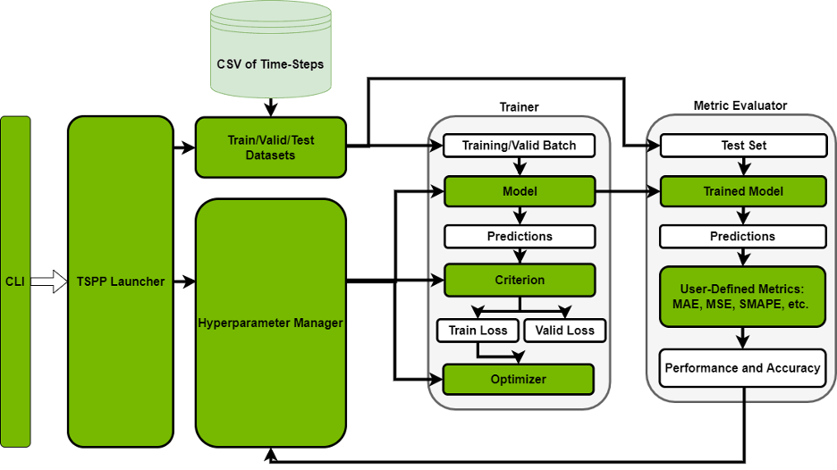
The forecasting system follows a structured approach with clear separation of concerns:

Each component is designed for modularity , scalability , and maintainability in real-world applications.

Our synthetic time series combines realistic temporal components to demonstrate neural network effectiveness on complex patterns:

git clone https://github.com/yourusername/time-series-neural-forecasting cd time-series-neural-forecasting pip install -r requirements.txt

# Import the main components from time_series_forecasting import generate_time_series , windowed_dataset , create_model # Generate synthetic time series TIME , SERIES = generate_time_series () # Create windowed dataset for training train_dataset = windowed_dataset ( series_train , window_size = 20 ) # Build and train the neural network model = create_model ( window_size = 20 ) history = model . fit ( train_dataset , epochs = 100 ) # Generate forecasts forecast = generate_forecast ( model , SERIES , window_size = 20 )

model = tf . keras . models . Sequential ([ tf . keras . Input ( shape = ( window_size ,)), tf . keras . layers . Dense ( 128 , activation = 'relu' ), tf . keras . layers . Dense ( 64 , activation = 'relu' ), tf . keras . layers . Dense ( 32 , activation = 'relu' ), tf . keras . layers . Dense ( 1 ) ])

def windowed_dataset ( series , window_size , shuffle = True ): # Create sliding windows for supervised learning dataset = tf . data . Dataset . from_tensor_slices ( series ) dataset = dataset . window ( window_size + 1 , shift = 1 , drop_remainder = True ) dataset = dataset . flat_map ( lambda window : window . batch ( window_size + 1 )) # Split into features and labels dataset = dataset . map ( lambda window : ( window [: - 1 ], window [ - 1 ])) # Apply shuffling and batching if shuffle : dataset = dataset . shuffle ( SHUFFLE_BUFFER_SIZE ) dataset = dataset . batch ( BATCH_SIZE ). prefetch ( 1 ) return dataset