Enquire Now
Medical Computer Vision · Clinical Diagnostics · PyTorch / TensorFlow · GPU Optimized · 2026

Real Estate Price Prediction Linear Regression Capstone

Tensor Pipeline · Custom Loss Formulations · Model Quantization · Accelerated Inference — A rigorous deep learning engineering project focused on automated pathological lesion segmentation and radiological disease classification. Architected for thesis defense viva presentations, IEEE reproduction, and high-throughput production deployment.

PyTorch
Core Framework
AMP FP16
Mixed Precision
TensorRT
Quantized Serving

Abstract

Real estate appraisal is a complex and important task, that can be made more precise and faster with the help of automated valuation tools. Usually the value of some property is determined by taking into account both structural and geographical characteristics. However, while geographical information is easily found, obtaining significant structural information requires the intervention of a real estate expert, a professional appraiser. In this paper we propose a Web data acquisition methodology, and a Machine Learning model, that can be used to automatically evaluate real estate properties. This method uses data from previous appraisal documents, from the advertised prices of similar properties found via Web crawling, and from open data describing the characteristics of a corresponding geographical area. We describe a case study, applicable to the whole Italian territory, and initially trained on a data set of individual homes located in the city of Turin, and analyze prediction and practical applicability.

real estate price prediction linear regression capstone Diagram
Figure: System Model & Simulation Flow for Real Estate Price Prediction Linear Regression Capstone

Keywords Real Estate Automated Valuation Models, Data Mining, Open Data, Ensemble Learning, Web Crawling

Introduction

The correct evaluation of house prices plays a fundamental role in our economy and affects all the participants to the

Real Estate Market, Including:

• professional appraisers, who are expert in the evaluation of properties and normally perform in loco visits and

Off-Site Paper Work;

• real estate appraisal companies, who request, harvest, standardise and verify the work of professional apprais-

Ers;

• financial institutions, needing to (1) set a justified property price prior to offering a mortgage loan or (2) evaluate a property portfolio, e.g. in the context of NPL (Non Performing Loan) management; • notaries/solicitors, needing to verify property values prior to guaranteeing the validity of some public transac- tion (e.g., a deed of purchase or the handling of inheritance issues); • home owners and buyers, and real estate agents, wanting to assess the reasonable market price of a property.

real estate price prediction linear regression capstone Diagram
Figure: System Model & Simulation Flow for Real Estate Price Prediction Linear Regression Capstone

A Preprint - September 4, 2019

In relatively recent years, the concept of an Automated Valuation Model (AVM) has emerged in this industry : an AVM is a software system, often based on online data and resources, that can produce a property evaluation in a semi-automatic way [2, 3, 1]. More recently, Artificial Intelligence and Machine Learning approaches to AVM construction have been adopted [4, 5, 6, 7, 8, 9]. This strategy is becoming increasingly useful in two wide areas of

Business Application:

• Appraisal professionals and companies produce a precise and authoritative evaluation, but with relatively high cost and time requirements - they can reduce such costs and times by using an AVM as a verification system (for the appraisal company) or as a helping tool (for the professional appraiser); • Some applications and stakeholders need a quick, or even real time property evaluation, that cannot be produced with the traditional process involving an expert. For example, a street-level bank office may want to immediately propose a draft mortgage offer to an incoming customer, before a formal expert appraisal is available.

When designing an AVM, one must consider the fact that the appraisal of a real estate property is a very difficult task, due to the high heterogeneity in both structural and geographical data. Moreover the price can be influenced by macroeconomic factors, that obviously change over time. In fact, the creation of a model able to predict real prices needs do deal with several problems caused by the complexity and the dynamics of the real estate market, and to the difficulty of obtaining reliable and objective data.

In this paper, in order to overcome these difficulties, we propose a type of AVM that (1) is adaptive, and uses Machine Learning methods to deal with the complexity and fast-changing characteristics of the real estate market, (2) finds links between diverse sources of data, including open data available on the Web, unstructured data that are obtained via Web Crawling, and private data from previous expert appraisals, and (3) is capable of producing real-time valuations.

A case study is provided, where this proposed Adaptive AVM is applied to the Italian residential real estate market. Three different approaches to feature selection and Machine Learning have been experimented with, yielding surprising results, where many features normally considered important have turned out to be irrelevant. We have used a set of previously appraised residential properties in Turin, Italy, obtaining additional relevant data from heterogeneous Web sources. The results, measured on independent test sets, have shown that the model is predictive and practically effective for the whole Italian territory.

Related Work And Innovations

Previous research on Automated Valuation Models for Real Estate has been initially led by so-called "hedonic" models [10, 11, 12, 13]. "Hedonic" literally suggests that the buying of the target property, and hence living in it, is a source of "pleasure". The better (and hence more expensive) the property, the higher this specific notion of real estate pleasure, stemming from property characteristics leading to such sensations: a nice view, proximity to services and pleasant life, the presence of an elevator, parking lots, a concierge. We will call all such pleasure-giving characteristics our "hedonic" features.

In older approaches hedonic features were mainly derived from intrinsic characteristics of the property, e.g. number of rooms and square meters, the number of bathrooms, the floor number. Again, in those traditional approaches, there was generally a linearity assumption - the value V (P) of some property P would depend linearly on the corresponding

(1)

where βi is the "i-th" coefficient, ϵ(P) is some correction to be applied to this particular property, and η is a property- independent correction that applies to some geographical perimeter or application context. In more recent research, a number of novelties come into place: • Non linear and even non-parametric models: we no longer assume the valuation depends linearly on the selected features, as in equation 1. Some studies suggest that this is not in fact the case for real estate valuations . In many cases, we just do not know what kind of dependency exists between the features and the sought valuation - we thus follow a non-parametric approach, where the type of regressor is unknown . In the present study we also follow this approach, and we do not assume linearity nor the correspondence to a particular form of classifier/regressor.

A Preprint - September 4, 2019

• Non-hedonic view. Some features are not necessarily "good" or "bad", but rather a part of a more complex analysis. For example, the predominance of foreigners in the neighborhood can lead to higher evaluations for small flats or near a metropolitan city center, while it could have opposed effects in the suburbs and for family houses. We follow this view in this paper, recognizing the complex nature of real estate appraisal.

• Implementation with AI and Machine Learning. The availability and increased performance of Machine Learning approaches has led to a widespread use of such technologies in AVMs for real estate [16, 2, 17, 7, 18, 19]. This includes the use of artificial neural networks [5, 20, 4, 21, 14], decision trees , random forests [1, 9, 22], gradient boosting and support vector machines . In the present paper we have also used Extremely Randomized Trees (Extra Trees) , that seem to perform well in this context. Finally, multi task learning has been used both for AVMs and for DOM (Days on the Market) prediction . Other AI techniques may be relevant, such as language classification and even semantic NLP for any text that can be referred to the property neighbourhoods. Image classification and recognition has also been used in the real estate AVM context .

• Extrinsic features from Web and open data. Not only the features directly related to the target property are important, but also the ones derived from neighbouring amenities and services, as well as linked to totally external information. Space and location-dependent external information has often been found to be important [17, 1]. Neighbouring area information has also been used, including criminality rate, population density and average income, pollution, services and transportation, and the distance from local river banks [16, 5, 6]. In the present study we address this issue in a structured and general way, by defining a notion of "point of interest" (PoI) concerning some subject or service (e.g., transportation, entertainment, sports). Such PoIs are sought for and geographically mapped, based on available open data (see "online resources" at the end of the paper: open data for the Turin municipality - "aperTO", see section 6 below, and nation-wide , Foursquare, Google Maps, OMI ). They are then linked to the target property based on distance and relevance, yielding an organized and comprehensive set of extrinsic features, that are added to the intrinsic features that are present in the appraisal data set1.

• Locally-oriented context. A number of approaches were tailored to a particular geographic area, or evaluated in such local perimeters, e.g. Montreal , Beijing [8, 25], London , Los Angeles , Hanoi , Zurich , Stockholm , Singapore , Italy (see [12, 30], as well as the present study), and Slovenia . This could be seen as a limitation, as if a general methodology was out of hand. Realistically, though, it makes very good sense because (1) valuation practices and regulations differ from one nation to another, (2) different kinds of open data are available and (3) good feature selection is essential and sets of best available features differ geographically. One important contribution of the present paper was to find out that some features obtained from OMI (see section 4.1 below) are essential for AVMs targeting the Italian territory.

In our approach, we also bring about another novelty, that we believe is not common in the literature. We started from a business and enterprise need, not a consumer-oriented view. For real estate appraisal company, the goal is to obtain a reasonable and expert-supported and validated valuation for some property. We do not target the actual deed of purchase price, nor are we interested in the advertised real estate agency price. As a consequence, we used a data set of expert valuations, not a set of example prices as obtained from Web advertisements, as, e.g., in [13, 9]. We however did use such advertised prices, and obtained them via crawling of specialized Web sites, but only as so-called "comparable" properties (see section 3.3 below), that are routinely used by appraisal experts as part of their valuation process.

As a consequence, our approach can be used as a basis for business services to appraisal companies and experts, because it is integrated into their processes and corresponds to their best practices. Moreover, based on our data sets and experiments, we have outperformed the best available results in this context , representing the current state of the art.

Data Set And Open Data Acquisition

For the purpose of this research we have used three different data sources: (1) a corpus of professional and validated property appraisal documents and corresponding data base, (2) geographical and open data obtained from heterogeneous public Web sources, and (3) advertised prices for comparable properties obtained via Web crawling. We discuss such data sources in the next subsections.

1It should be noted that such PoI indexes can be weighted based on particular valuation contexts or specific target populations, e.g. young people (who could be more interested in public transportation and entertainment), or families (who could be more interested

Data Set Of Available Appraisals

The data used to perform the analysis was provided by a multinational real estate appraisal company, with a subsidiary having significant activities in Italy. The initial data set consisted of 7988 property valuations, performed by professional appraisers, and validated by the company. These properties are all located in the city of Turin, and the valuations were performed between 2011 and 2016. The full set of available information for each property is summarized in Table 1, and the distribution of target valuations in the appraisal data set is shown in Fig. 1.

As a first step, this data set was anonymized, removing personal buyer or mortgage application information, as well as bank details.

Valuation

Table 1: Information in the available appraisal data set For the most important variables in Table 1, we observe the following: • Valuation: valuation in Euros, as assessed by a professional appraiser and stored in the appraisal document.

This is the target variable, i.e. the value we will want to predict and the output of our AVM when we will use it on new, yet to be evaluated properties. • City Area: Central, Near-central, Larger City Boundary, Suburbs

• Number Of Bathrooms: 0 To 7, Mean Value = 1.2

• Surface: 40.4 to 249 square meters, mean value = 94.7

• Floor: -1 To 11, Mean Value = 3

• Registered use: based on the Italian land register ("catasto"), the possible values include, e.g., "residential", "office", "warehouse". This data set contained a wealth of information, that is normally difficult to acquire in such quantity and detail. However, it was too diversified and a data cleaning and selection process was performed. In particular: • in order to have an omogeneous data set, we only considered properties with a "residential" registered use, because this was the most common case; by contrast, properties with different registered uses are difficult to

Compare;

• we excluded houses with a surface greater than 250 square meters, as they are rare and belong to a peculiar

Market Sector;

• we only considered houses with a global valuation between 20, 000 C and 700, 000 C, as the other cases are

Considered Exceptional For The Same Reasons;

• we also excluded the valuations of complex properties, as for example houses with a garage, because of their limited number and more complex description structure. After this selection process, the 7988 valuations were reduced to 3983, still a significant number for our practical purposes and prediction targets.

Density

Figure 1: Valuation distribution in the Appraisal Data Set Finally, we performed a feature standardisation activity. For example, some features where normalized so as to have values between -1 and 1, e.g. construction year and floor, so as to make them easier to process in subsequent phases.

Geographical And Open Data

Using information available on the Web, indexed with the geographical location of the properties, we have extended the features contained in the appraisal data set, with new and useful information. This consists mainly of two data categories: OMI areas and values, and nearby area information.

Omi Areas

The Italian Revenue Agency is responsible of the OMI ("Osservatorio del Mercato Immobiliare" - Italian Real-Estate Observatory ), see links in Section 6. For each registered use of properties, the surface of each Italian municipality is divided into different areas, called OMI areas, having homogeneous real-estate characteristics and valuation schemes.

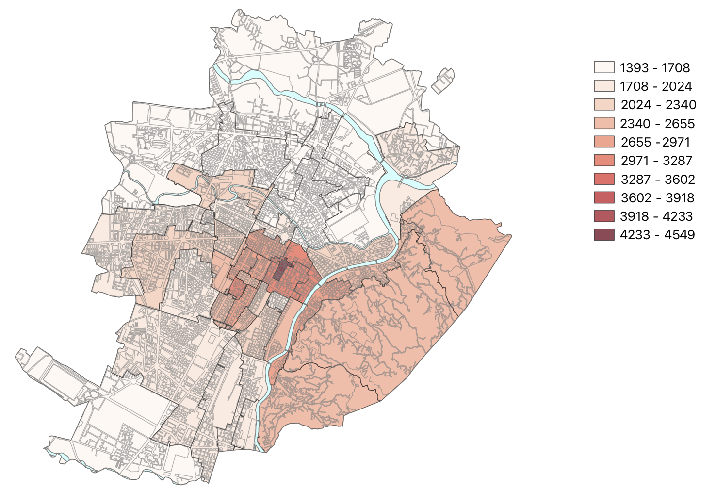
Every six months, OMI provides an update of the price range (minimum and maximum price), for each OMI area. For example, Fig. 2 provides a graphical representation of the 41 OMI areas in the municipality of Turin, with the corresponding average prices. For the purpose of easier comparison, we report next, in Fig. 3, the valuations as predicted by our AVM - as it can be seen the predicted prices are quite close to the actual values. The price ranges in an OMI zone may vary according to the dynamics of the real estate market or to specific changes regarding some geographic location. The OMI area associated to some property may be obtained from OMI, using its geographical coordinates.

OMI also provides the formal description of "polygons" that define the OMI areas (see again Section 6 below). We have followed two different approaches in this research. In the first approach (OMI names), we used the name of the OMI area as an additional, constructed feature. This has some drawbacks. First, as previously explained, the price range in a specific OMI area may change over time. This implies that if the model has been trained using valuations performed in a certain period of time, the valuation of a new property in the future could be affected by the changes of price in the corresponding OMI area. Second, the feature will be effective only in the valuation of properties that were located in OMI areas that are represented in the training set.

Another issue could be represented by the creation of new OMI areas or the disappearance of old OMI areas over time. Finally, by using the OMI area name, a discrete value, we lose important geographical information, such as the distance between different OMI areas.

In the second approach (OMI min/max values), we introduce as new features the upper and the lower limit of the price range of the OMI area at the time of the appraisal. The idea behind this choice is that of separating the model from specific OMI areas, trying to transform the OMI area name into ordinal features. As the criteria used by OMI for the creation of the price range are the same for each municipality and remain constant over time, this choice allows us to use the model to evaluate properties located in OMI areas not even contained in the training set, and to perform evaluations long after its creation.

We have performed experiments with both feature construction approaches, and the latter (OMI min/max values) has produced superior results, as discussed later.

A Preprint - September 4, 2019

Figure 2: Graphical representation of the Turin real estate data set divided by OMI area - average prices Figure 3: Graphical representation of the Turin real estate data set divided by OMI area - predicted prices

3.2.2

Nearby area information (Points of Interest - PoI) Starting from the geographical position of the property (latitude, longitude), as contained in the appraisal data, we construct new features using open data available from the Web, and related to corresponding surrounding areas (nearby areas). In particular, we built a set of so called "Points of Interest" (PoI). Points of interest correspond to activities and resources that are present in the territory, are geolocalized, and have a potential positive influence on the price of surrounding properties. This corresponds to best practices in real estate appraisal, where experts normally produce valuation reports that include features such as nearby metro and bus stops, schools, and museums. We have grouped our PoIs into 13 categories: Arts, Business&Services, Entertainment, Food&Beverage, Healthcare&Wellness, Instruction, Landmarks, Religious services, Retail, Security, Sport&Recreation, Transportation, Travel. A data set of PoIs has been created by aggregating information from Foursquare, Google Maps and the Turin Open Data "AperTo" Web Site (see Section 6). The idea is to construct a new property feature for each PoI category, by counting the number of PoIs in that category that are within a threshold distance. However, in order to avoid the on/off effect of a strict threshold, we define 4 circles around the property, and associate descending weights to the PoIs falling within these circles, thus giving more importance to the PoIs that are closer to the property. We obtain the following formula, defining the property feature fj

A Preprint - September 4, 2019

where dk, is the distance of the property from PoI number k in the jth category, and r is a threshold distance, initially set at 1 km. Finally, and additional feature was used, defined simply as the distance from the city center, a special kind of PoI.

Comparable Properties

According to best appraisal practices in Italy, the expert’s valuation document normally comprises a description and identification of so-called "comparable properties", i.e. properties that are geographically near the target property and have similar characteristics. The price per square meter will then be similar and the professional appraiser will use it as an important starting point in order to reach a final valuation. Professional appraisers can obtain some such comparable property data from the appraisal company’s database of previous valuations. They cannot use purchase deeds from notaries as this is not publicly available in Italy (as it is in France, and, partially, in the UK). Using previous appraisal company valuations will however introduce some bias, as the same experts and the same company standards were used.

In recent years, appraisers also use real estate offers as advertised on the Web. There are many such publicly available services in Italy, offered to real estate agents as well as private individuals, that allow for sophisticated search interrogations, that may be filtered by, e.g., distance from a specified location, property type, price range, floor, maintenance status. The expert can then download the advertised property description and include a selection of relevant data in her valuation document. The advertised price of such comparable properties will also be used as a reference in setting the valuation of the target property. It must be noted, however, that the advertised price is not a sale price, but rather an upper bound, awaiting further negotiations. The expert will then have to take this simple truth into account when using the advertised price as an input.

In our approach, we have simulated the above expert best practices for comparable data acquisition, while letting Machine Learning do the rest and decide how to use such data. In particular, our system is able to acquire three distinct

Types Of Comparable Properties:

• properties that are the target of previous appraisals in the data set: we have such data available in a structured data base, and the corresponding valuation is labeled as a "comparable property valuation price", as it was produced by some appraisal expert some time in the past - the corresponding valuation date is stored and

Should Be Taken Into Account;

• properties that are cited as comparable in previous appraisal documents: this is available in the expert’s text document, and not in the data base, so we were not able to extract it easily - we did not use this at the present

Time;

• properties that are advertised for sale on the Web. For the latter category of comparable properties, we simulated the behaviour of the expert using a controlled Web Crawling strategy, where a limited number of properties is sought near the target property. If too many properties are found, the distance threshold is reduced and additional filters are set, with the purpose of finding properties that have similar characteristics (e.g. floor and maintenance status). If the demonstrator is scaled up and used in a production and commercial service, a number of issues will have to be addressed, including legal concerns about the use of a robot to retrieve possibly proprietary information (though actually publicly available on the Web). Some technical issues should also be analyzed, such as dealing with anti-automation (e.g., Captchas), and robot detection/classification . Finally, frequent Web format changes in real estate portals will require manual Crawler adaptation - again, legal issues should be addressed here.

The demonstrator is now able to retrieve a set number of comparable properties as described above, with corresponding attributes and advertised or valuated price. The result of the process is a new constructed feature for the target property: the average price per square meter of comparable properties.

Machine Learning Methodology

We will now describe how the described data set was used, in order to train our AVM. First we will describe three different approaches that we have used for feature selection, and subsequently we will describe how the data set was partitioned and which Machine Learning algorithms were used.

Feature Selection

The data set described in the previous section is complex and involves significant amounts of correlated information. We have followed three distinct approaches to the use of such data, by selecting different subsets of the available features:

Ai Adaptive Learning

This project focuses on ai adaptive learning using modern AI and machine learning techniques. The content below is adapted from research literature and practical implementation notes.

We propose a novel high-performance and interpretable canon-

addition, unlike tree learning, DNNs enable gradient descent- ical deep tabular data learning architecture, TabNet. TabNet based end-to-end learning for tabular data which can have a uses sequential attention to choose which features to reason multitude of benefits: (i) efficiently encoding multiple data from at each decision step, enabling interpretability and more types like images along with tabular data; (ii) alleviating the efficient learning as the learning capacity is used for the most need for feature engineering, which is currently a key aspect

salient features. We demonstrate that TabNet outperforms in tree-based tabular data learning methods; (iii) learning other variants on a wide range of non-performance-saturated from streaming data and perhaps most importantly (iv) end- tabular datasets and yields interpretable feature attributions to-end models allow representation learning which enables plus insights into its global behavior. Finally, we demonstrate many valuable application scenarios including data-efficient

self-supervised learning for tabular data, significantly improv- domain adaptation (Goodfellow, Bengio, and Courville 2016), ing performance when unlabeled data is abundant. generative modeling (Radford, Metz, and Chintala 2015) and

Introduction We propose a new canonical DNN architecture for tabular

Deep neural networks (DNNs) have shown notable success data, TabNet. The main contributions are summarized as: efficiently encode the raw data into meaningful representa- enabling flexible integration into end-to-end learning. tions, fuel the rapid progress. One data type that has yet to 2. TabNet uses sequential attention to choose which fea- see such success with a canonical architecture is tabular data. tures to reason from at each decision step, enabling in-

Despite being the most common data type in real-world AI terpretability and better learning as the learning capacity (as it is comprised of any categorical and numerical features), is used for the most salient features (see Fig. 1). This under-explored, with variants of ensemble decision trees for each input, and unlike other instance-wise feature se- Why? First, because DT-based approaches have certain bene- and van der Schaar 2019), TabNet employs a single deep

fits: (i) they are representionally efficient for decision mani- learning architecture for feature selection and reasoning. folds with approximately hyperplane boundaries which are 3. Above design choices lead to two valuable properties: (i) common in tabular data; and (ii) they are highly interpretable TabNet outperforms or is on par with other tabular learn- in their basic form (e.g. by tracking decision nodes) and there ing models on various datasets for classification and re-

are popular post-hoc explainability methods for their ensem- gression problems from different domains; and (ii) TabNet ble form, e.g. (Lundberg, Erion, and Lee 2018) – this is an enables two kinds of interpretability: local interpretability important concern in many real-world applications; (iii) they that visualizes the importance of features and how they are fast to train. Second, because previously-proposed DNN are combined, and global interpretability which quantifies

architectures are not well-suited for tabular data: e.g. stacked the contribution of each feature to the trained model. convolutional layers or multi-layer perceptrons (MLPs) are 4. Finally, for the first time for tabular data, we show signif- vastly overparametrized – the lack of appropriate inductive icant performance improvements by using unsupervised bias often causes them to fail to find optimal solutions for tab- pre-training to predict masked features (see Fig. 2).

ular decision manifolds (Goodfellow, Bengio, and Courville

Why is deep learning worth exploring for tabular data?

One obvious motivation is expected performance improve- Feature selection: Feature selection broadly refers to judi- Copyright © 2021, Association for the Advancement of Artificial ciously picking a subset of features based on their useful-

Professional occupation related Investment related

Feedback from Feedback to

Feature selection Input processing Feature selection Input processing

previous step next step … …

Predicted output (whether the income level >$50k)

selection enables interpretability and better learning as the capacity is used for the most salient features. TabNet employs multiple decision blocks that focus on processing a subset of input features for reasoning. Two decision blocks shown as examples process features that are related to professional occupation and investments, respectively, in order to predict the income level.

Unsupervised pre-training Supervised fine-tuning

Age Cap. gain Education Occupation Gender Relationship Age Cap. gain Education Occupation Gender Relationship 5 2000 ? Exec-managerial F Wife 6 2000 Bachelors Exec-managerial M Husband 1 0 ? Farming-fishing M ? 2 0 High-school Farming-fishing M Unmarried

? 50 Doctorate Prof-specialty M Husband 4 50 Doctorate Prof-specialty M Husband 2 ? ? Handlers-cleaners F Wife 2 0 High-school Handlers-cleaners F Wife 5 3000 Bachelors ? ? Husband 5 3000 Bachelors Exec-managerial M Husband

3 0 Bachelors ? F ? 3 100 Bachelors Prof-specialty F Wife ? 0 High-school Armed-Forces ? Husband 2 0 High-school Armed-Forces M Husband

TabNet decoder Decision making

Age Cap. gain Education Occupation Gender Relationship Income > $50k

3 M False

level can be guessed from the occupation, or the gender can be guessed from the relationship. Unsupervised representation learning by masked self-supervised learning results in an improved encoder model for the supervised learning task.

ward selection and Lasso regularization (Guyon and Elisseeff performance with compact representations. 2003) attribute feature importance based on the entire training Tree-based learning: DTs are commonly-used for tabular data, and are referred as global methods. Instance-wise fea- data learning. Their prominent strength is efficient picking ture selection refers to picking features individually for each of global features with the most statistical information gain

to maximize the mutual information between the selected mance of standard DTs, one common approach is ensembling features and the response variable, and in (Yoon, Jordon, and to reduce variance. Among ensembling methods, random van der Schaar 2019) by using an actor-critic framework to forests (Ho 1998) use random subsets of data with randomly mimic a baseline while optimizing the selection. Unlike these, selected features to grow many trees. XGBoost (Chen and

sity in end-to-end learning – a single model jointly performs recent ensemble DT approaches that dominate most of the feature selection and output mapping, resulting in superior recent data science competitions. Our experimental results

!# + Softmax !" < % !" > % !# > & !# > &

ReLU ReLU &

$" !" − $" % −1 −$" !" + $" % −1 −1 $# !# − $# & % −1 −$# !# + $# & !"

FC FC

W: [$" , - $" , 0, 0] W: [0, 0, $# , - $# ] !" < % b: [-a $" , a $" , -1, -1] b: [-1, -1, -d $# , d $# ] !# < & !" > % !# < & [!" ] [!# ]

M: [1, 0] M: [0, 1]

(right). Relevant features are selected by using multiplicative sparse masks on inputs. The selected features are linearly transformed, and after a bias addition (to represent boundaries) ReLU performs region selection by zeroing the regions. Aggregation of multiple regions is based on addition. As C and C get larger, the decision boundary gets sharper.

for various datasets show that tree-based models can be out- constructs a sequential multi-step architecture, where each performed when the representation capacity is improved with step contributes to a portion of the decision based on the deep learning while retaining their feature selecting property. selected features; (iii) improves the learning capacity via non- Integration of DNNs into DTs: Representing DTs with linear processing of the selected features; and (iv) mimics

DNN building blocks as in (Humbird, Peterson, and McClar- ensembling via higher dimensions and more steps. ren 2018) yields redundancy in representation and ineffi- cient learning. Soft (neural) DTs (Wang, Aggarwal, and Liu Fig. 4 shows the TabNet architecture for encoding tabu- functions, instead of non-differentiable axis-aligned splits. mapping of categorical features with trainable embeddings.

However, losing automatic feature selection often degrades We do not consider any global feature normalization, but performance. In (Yang, Morillo, and Hospedales 2018), a soft merely apply batch normalization (BN). We pass the same D- binning function is proposed to simulate DTs in DNNs, by dimensional features f ∈ <B×D to each decision step, where 2019) proposes a DNN architecture by explicitly leveraging multi-step processing with Nsteps decision steps. The ith

expressive feature combinations, however, learning is based step inputs the processed information from the (i − 1)th step on transferring knowledge from gradient-boosted DT. (Tanno to decide which features to use and outputs the processed ing from primitive blocks while representation learning into sion. The idea of top-down attention in the sequential form edges, routing functions and leaf nodes. TabNet differs from is inspired by its applications in processing visual and text

these as it embeds soft feature selection with controllable data (Hudson and Manning 2018) and reinforcement learn- Self-supervised learning: Unsupervised representation relevant information in high dimensional input. learning improves supervised learning especially in small Feature selection: We employ a learnable mask M[i] ∈ has shown significant advances – driven by the judicious capacity of a decision step is not wasted on irrelevant

choice of the unsupervised learning objective (masked input ones, and thus the model becomes more parameter effi- prediction) and attention-based deep learning. cient. The masking is multiplicative, M[i] · f . We use an attentive transformer (see Fig. 4) to obtain the masks us- TabNet for Tabular Learning ing the processed features from the preceding step, a[i − 1]:

M[i] = sparsemax(P[i − 1] · hi (a[i − 1])). Sparsemax nor-

DTs are successful for learning from real-world tabular malization (Martins and Astudillo 2016) encourages sparsity datasets. With a specific design, conventional DNN building by mapping the Euclidean projection onto the probabilistic blocks can be used to implement DT-like output manifold, simplex, which is observed to be superior in performance and e.g. see Fig. 3). In such a design, individual feature selec- aligned with the goal of sparse feature selection for explain-

tion is key to obtain decision boundaries in hyperplane form, PD which can be generalized to a linear combination of features ability. Note that j=1 M[i]b,j = 1. hi is a trainable func- where coefficients determine the proportion of each feature. tion, shown in Fig. 4 using a FC layer, followed by BN. P[i] TabNet is based on such functionality and it outperforms DTs is the prior scale term, denoting how much a particular feature

Qi while reaping their benefits by careful design which: (i) uses has been used previously: P[i] = j=1 (γ − M[j]), where γ sparse instance-wise feature selection learned from data; (ii) is a relaxation parameter – when γ = 1, a feature is enforced

+ Softmax

Feature Feature …

transformer transformer

x Nsteps Features

+ Softmax

Feature …

transformer transformer Feature Feature Feature Feature transformer

Encoded representation

transformer transformer Attentive transformer … Mask transformer …

Step 2 Decision step dependent

transformer transformer

BN Feature Feature

FC BN transformer transformer

+ 0.5 0.5 0.5 Agg. Agg. Features Features FC FC + +

Reconstructed + … Feature attributes + … features

(a) TabNet encoder architecture (b) TabNet decoder architecture Feature transformer Feature Attentive transformer Shared across decision steps Decision step dependent transformer GLU

Decision step dependent Prior scales

+ 0.5 0.5 0.5

0.5 0.5 0.5

+ Attentive transformer (c) (d)

Prior scales

divides the processed representation to be used by the attentive transformer of the subsequent step as well as for the overall Attentive BN FC

output. For each step, the feature selection mask provides interpretable information about the model’s functionality, and the +

masks can be aggregated to obtain global feature transformer important attribution. (b) TabNet decoder, composed of a feature transformer block at each step. (c) A feature transformer block example – 4-layer network is shown, where 2 are shared across all decision

Prior scales

steps and 2 are decision step-dependent. Each layer is composed of a fully-connected (FC) layer, BN and GLU nonlinearity. (d) +

An attentive transformer block example – a single layer mapping is modulated with a prior scale information which aggregates Sparsemax

how much each feature has been used before the current decision step. sparsemax (Martins and Astudillo 2016) is used for BN FC

normalization of the coefficients, resulting in sparse selection of the salient features. +

to be used only at one decision step and as γ increases, more propose the aggregate.feature importance mask, Magg−b,j = flexibility is provided to use a feature at multiple decision PNsteps ηb [i]Mb,j [i]

PD PNsteps

ηb [i]Mb,j [i].2 i=1 i=1 steps. P is initialized as all ones, 1B×D , without any prior j=1

on the masked features. If some features are unused (as in self- Tabular self-supervised learning: We propose a decoder supervised learning), corresponding P entries are made 0 architecture to reconstruct tabular features from the Tab- to help model’s learning. To further control the sparsity of the Net encoded representations. The decoder is composed of selected features, we propose sparsity regularization in the feature transformers, followed by FC layers at each deci-

form of entropy (Grandvalet and Bengio 2004), Lsparse = sion step. The outputs are summed to obtain the recon-

PNsteps PB PD −Mb,j [i] log(Mb,j [i]+)

i=1 b=1 j=1 Nsteps ·B , where  is a structed features. We propose the task of prediction of miss- small number for numerical stability. We add the sparsity reg- ing feature columns from the others. Consider a binary mask ularization to the overall loss, with a coefficient λsparse . Spar- S ∈ {0, 1}B×D . The TabNet encoder inputs (1 − S) · f̂ sity provides a favorable inductive bias for datasets where and the decoder outputs the reconstructed features, S · f̂ . We

most features are redundant. initialize P = (1 − S) in encoder so that the model em- Feature processing: We process the filtered features using phasizes merely on the known features, and the decoder’s last a feature transformer (see Fig. 4) and then split for the FC layer is multiplied with S to output the unknown features. decision step output and information for the subsequent We consider the reconstruction loss in self-supervised phase:

step, [d[i], a[i]] = fi (M[i] · f ), where d[i] ∈ <B×Nd and 2

PB PD (f̂b,j −fb,j )·Sb,j

a[i] ∈ <B×Na . For parameter-efficient and robust learning b=1 j=1

√ PB PB 2

. Normalization b=1 (fb,j −1/B b=1 fb,j ) with high capacity, a feature transformer should comprise layers that are shared across all decision steps (as the same with the population standard deviation of the ground truth features are input across different decision steps), as well as is beneficial, as the features may have different ranges. We decision step-dependent layers. Fig. 4 shows the implementa- sample Sb,j independently from a Bernoulli distribution with

tion as concatenation of two shared layers and two decision parameter ps , at each iteration. step-dependent layers. Each FC layer is followed by BN and eventually connected to a normalized residual √ connection We study TabNet in wide range of problems, that contain with normalization. Normalization with 0.5 helps to sta- regression or classification tasks, particularly with published bilize learning by ensuring that the variance throughout the benchmarks. For all datasets, categorical inputs are mapped

For faster training, we use large batch sizes with BN. Thus, bedding and numerical columns are input without and pre- except the one applied to the input features, we use ghost BN processing.4 We use standard classification (softmax cross (Hoffer, Hubara, and Soudry 2017) form, using a virtual batch entropy) and regression (mean squared error) loss functions size BV and momentum mB . For the input features, we ob- and we train until convergence. Hyperparameters of the Tab-

serve the benefit of low-variance averaging and hence avoid Net models are optimized on a validation set and listed in ghost BN. Finally, inspired by decision-tree like aggregation Appendix. TabNet performance is not very sensitive to most as in Fig. 3, we construct the overall decision embedding hyperparameters as shown with ablation studies in Appendix. as dout = i=1 PNsteps ReLU(d[i]). We apply a linear mapping In Appendix, we also present ablation studies on various de-

Wfinal dout to get the output mapping.1 sign and guidelines on selection of the key hyperparameters. Interpretability: TabNet’s feature selection masks can shed For all experiments we cite, we use the same training, val- light on the selected features at each step. If Mb,j [i] = 0, idation and testing data split with the original work. Adam optimization algorithm (Kingma and Ba 2014) and Glorot then j th feature of the bth sample should have no contribution uniform initialization are used for training of all models.5

to the decision. If fi were a linear function, the coefficient

Mb,j [i] would correspond to the feature importance of fb,j . Instance-wise feature selection

Although each decision step employs non-linear processing, their outputs are combined later in a linear way. We aim Selection of the salient features is crucial for high perfor- to quantify an aggregate feature importance in addition to mance, especially for small datasets. We consider 6 tabular requires a coefficient that can weigh the relative importance samples). The datasets are constructed in such a way that of each step in the decision. We simply propose ηb [i] = only a subset of the features determine the output. For Syn1-

PNd Syn3, salient features are same for all instances (e.g., the

c=1 ReLU(db,c [i]) to denote the aggregate decision con- tribution at ith decision step for the bth sample. Intuitively, if 2

Normalization is used to ensure D

P j=1 Magg−b,j = 1. db,c [i] < 0, then all features at ith decision step should have 3

0 contribution to the overall decision. As its value increases, prove the performance, but interpretation of individual dimensions

it plays a higher role in the overall linear combination. Scal- may become challenging. ing the decision mask at each decision step with ηb [i], we Specially-designed feature engineering, e.g. logarithmic trans- formation of variables highly-skewed distributions, may further

For discrete outputs, we additionally employ softmax during

training (and argmax during inference). An open-source implementation will be released.

Global: using only globally-salient features, Tree Ensembles (Geurts, Ernst, and Wehenkel 2006), Lasso-regularized model, L2X

Syn Syn Syn Syn Syn Syn

No selection .5 ± .0 .7 ± .0 .8 ± .0 .5 ± .0 .6 ± .0 .6 ± .0 Tree .5 ± .1 .8 ± .0 .8 ± .0 .6 ± .0 .7 ± .0 .7 ± .0 Lasso-regularized .4 ± .0 .5 ± .0 .8 ± .0 .5 ± .0 .6 ± .0 .7 ± .0

INVASE .6 ± .0 .8 ± .0 .9 ± .0 .7 ± .0 .7 ± .0 .8 ± .0

Global .6 ± .0 .8 ± .0 .9 ± .0 .7 ± .0 .7 ± .0 .8 ± .0 TabNet .6 ± .0 .8 ± .0 .8 ± .0 .7 ± .0 .7 ± .0 .8 ± .0

output of Syn depends on features X -X ), and global fea- Table 3: Performance for Poker Hand induction dataset. ture selection, as if the salient features were known, would give high performance. For Syn4-Syn6, salient features are Model Test accuracy (%) instance dependent (e.g., for Syn4, the output depends on ei- DT 50.0 ther X -X or X -X depending on the value of X ), which MLP 50.0

makes global feature selection suboptimal. Table 1 shows that Deep neural DT 65.1

TabNet outperforms others (Tree Ensembles (Geurts, Ernst, XGBoost 71.1

and Wehenkel 2006), LASSO regularization, L2X (Chen LightGBM 70.0 van der Schaar 2019). For Syn1-Syn3, TabNet performance TabNet 99.2 is close to global feature selection - it can figure out what Rule-based 100.0 features are globally important. For Syn4-Syn6, eliminating instance-wise redundant features, TabNet improves global feature selection. All other methods utilize a predictive model Poker Hand (Dua and Graff 2017): The task is classifica-

with 43k parameters, and the total number of parameters is tion of the poker hand from the raw suit and rank attributes of 101k for INVASE due to the two other models in the actor- the cards. The input-output relationship is deterministic and critic framework. TabNet is a single architecture, and its size hand-crafted rules can get 100% accuracy. Yet, conventional is 26k for Syn1-Syn and 31k for Syn4-Syn6. The compact DNNs, DTs, and even their hybrid variant of deep neural DTs

representation is one of TabNet’s valuable properties. (Yang, Morillo, and Hospedales 2018) severely suffer from the imbalanced data and cannot learn the required sorting and Performance on real-world datasets ranking operations (Yang, Morillo, and Hospedales 2018).

Tuned XGBoost, CatBoost, and LightGBM show very slight

as it can perform highly-nonlinear processing with its depth, Model Test accuracy (%) without overfitting thanks to instance-wise feature selection.

CatBoost 85.1 Table 4: Performance on Sarcos dataset. Three TabNet mod-

AutoML Tables 94.9 els of different sizes are considered.

Forest Cover Type (Dua and Graff 2017): The task is clas- MLP 2.1 0.14M

sification of forest cover type from cartographic variables. Adaptive neural tree 1.2 0.60M approaches that are known to achieve solid performance (AutoML 2019), an automated search framework based on TabNet-M 0.2 0.59M ensemble of models including DNN, gradient boosted DT, TabNet-L 0.1 1.75M with very thorough hyperparameter search. A single TabNet without fine-grained hyperparameter search outperforms it. Sarcos (Vijayakumar and Schaal 2000): The task is re-

gressing inverse dynamics of an anthropomorphic robot arm.

very small model is possible with a random forest. In the very and TabNet merely focuses on the relevant ones. For Syn4, small model size regime, TabNet’s performance is on par the output depends on either X -X or X -X depending parameters. When the model size is not constrained, TabNet feature selection – it allocates a mask to focus on the indi- achieves almost an order of magnitude lower test MSE. cator X , and assigns almost all-zero weights to irrelevant

features (the ones other than two feature groups). models are denoted with -S and -M. Real-world datasets: We first consider the simple task of mushroom edibility prediction (Dua and Graff 2017). Tab- Model Test acc. (%) Model size Net achieves 100% test accuracy on this dataset. It is indeed Sparse evolutionary MLP 78.4 81K known (Dua and Graff 2017) that “Odor” is the most discrim-

What is this project about?

This project covers practical implementation and research aspects of the topic using AI/ML techniques.