Composite Repair Patch Ansys

Publication Reference Data:

Engineering, May 2016. Keywords: Composite patches, marine repairs, adhesive bonding, fatigue behaviour, bimaterial

Στην Οικογένειά Μου Και Τη Χριστίνα

also someone whom I have not met before and who proved to be a young Lecturer in Mechanical enjoy it!” which, I have to admit, found rather corny at the time. Looking back, I will have to agree with him, journeys, it involved frustration, tiredness, and dead ends but at the same time achievements, personal progress and beautiful moments. Albeit this was a personal endeavour it was far from lonely, and it would have been impossible to bring it to its present form without the support of the following people.

Firstly, I would like to express my deepest gratitude to my advisor Prof. Tsouvalis for offering me the during my Diploma Thesis and postgraduate studies are greatly treasured. He is largely responsible for shaping my scientific perception and has been a role model for me both as a tutor and as a person.

cooperation and for offering valuable assistance in the experimental activities, and the Co-Patch project partners for their efforts and inputs during the research project. Chatzidouros and Mr. Elias Kotsidis for all the discussions we had, their support and their encouragement throughout this endeavour. But foremost for their sincere friendship and everything we shared through all these years.

Denmark for providing me the opportunity to join his team and for his understanding when I was finalising my had concerning bimaterial fracture mechanics. Last but not least, I thank my family and my girlfriend Christina for their endless support and encouragement when I needed it most throughout this endeavour and for having them in my life.

Asileios A. Karatzas

Assessment and Design of Composite Patch Repairing in

Abstract

of defected marine steel structures. This work is the result of a combined experimental, numerical and analytical approach aiming at providing insight on the design, inspection and in service performance of such repairs. A design evaluation procedure has been developed based on simple analytical tools which are to be utilized by engineers for the design and analysis of composite patch repairing and other similar adhesively bonded applications.

A series of midscale static tests have been performed in defected steel plates, namely in corroded and notched plates. All plates have been repaired with composite patches and tested in tension. Additionally, different health monitoring and inspection methods have been applied to assess the quality of the repair both after installation and during operating conditions. Moreover, the effect of different aging scenarios has been investigated. Finally, 2D and 3D finite element models have been created using cohesive zone modelling which are in good agreement with the experimental findings.

Simultaneously, cracked plates on which composite patches have been installed were experimentally investigated under fatigue loading. Once again, apart from the efficiency of the repair, health monitoring and the effect of different aging scenarios have been assessed. Additionally, a methodology for the assessment of cracked elements in marine structures and the effectiveness of the investigated repair method is proposed. This methodology is based on the implementation of the common structural rules with the use of user subroutines and finite element modelling.

At the end of this work, emphasis is given in the use of linear fracture mechanics in bimaterial interfaces and a parametric study has been performed to quantify how key parameters affect the adhesive bond between the patch and the steel substrate. Following the parametric study, a simple, time effective design evaluation procedure for this kind of repairs is proposed.

structures, having addressed critical issues associated with their effectiveness and durability, and proposing a simple analytical procedure for their design.

Περιληψη

Η παρούσα διδακτορική διατριβή πραγματεύεται τη χρήση επιθεμάτων από σύνθετα υλικά για την επιδιόρθωση ατελειών που εμφανίζονται σε χαλύβδινες θαλάσσιες κατασκευές. Η εκπονηθείσα διατριβή είναι το αποτέλεσμα του συνδυασμού πειραματικής, αριθμητικής και αναλυτικής προσέγγισης. Στόχος της είναι η εκτίμηση της αποτελεσματικότητας της συγκεκριμένης μεθόδου επισκευής, η διερεύνηση τεχνικών επιθεώρησης της ακεραιότητάς της και τέλος η ανάπτυξη μίας απλής μεθοδολογία ελέγχου για τον ορθό σχεδιασμό αυτής.

Για να επιτευχθούν οι προαναφερθέντες στόχοι πραγματοποιήθηκε μία σειρά στατικών πειραματικών δοκιμών μεσαίας κλίμακας σε χαλύβδινες πλάκες που έφεραν εγκοπή και σε πλάκες που είχαν υποστεί διάβρωση. Όλα τα δοκίμια δοκιμάστηκαν σε εφελκυσμό. Ταυτόχρονα, εφαρμόστηκαν διαφορετικές μέθοδοι ελέγχου και παρακολούθησης για την αξιολόγηση της επισκευής και για τη μελέτη του τρόπου αστοχίας της.

Μέσω των πειραμάτων εξετάστηκε και η επίδραση της περιβαλλοντικής γήρανσης λαμβάνοντας υπόψη διαφορετικά σενάρια γήρανσης. Εν συνεχεία αναπτύχθηκαν δισδιάστατα και τρισδιάστατα μη γραμμικά μοντέλα πεπερασμένων στοιχείων με στόχο την αναπαραγωγή των πειραματικών αποτελεσμάτων. Τα αριθμητικά αποτελέσματα ήταν σε καλή συμφωνία με τις πειραματικές μετρήσεις.

Επιπρόσθετα, διεξήχθησαν δοκιμές κόπωσης σε χαλύβδινες πλάκες που έφεραν κεντρική ρωγμή και είχαν επιδιορθωθεί με επιθέματα από σύνθετα υλικά. Αντίστοιχα με τις στατικές δοκιμές, πέραν της αποτελεσματικότητας της μεθόδου, δόθηκε βάρος στην επίδραση της περιβαλλοντικής γήρανσης και στην εφαρμογή μεθόδων μη καταστρεπτικού ελέγχου για την αξιολόγηση του δεσμού μεταξύ του επιθέματος και της πλάκας. Επιπρόσθετα προτάθηκε μία αριθμητική μεθοδολογία αξιολόγησης τόσο της κρισιμότητας ρωγμών σε πλοία μεταφοράς πετρελαίου, καθώς και της μεθόδου επισκευής.

Στο τελευταίο τμήμα της διδακτορικής διατριβής δίνεται έμφαση στη χρήση της γραμμικά ελαστικής θεωρίας θραυστομηχανικής για διεπιφάνειες. Συγκεκριμένα, συνδυάζοντας αριθμητικά μοντέλα και αναλυτικούς τύπους πραγματοποιήθηκε παραμετρική μελέτη για να διερευνηθούν πως το μέτρο ελαστικότητας και το πάχος του επιθέματος σε σχέση με αυτό της μεταλλικής κατασκευής επιδρούν στην αποτελεσματικότητα της επισκευής υπό διαφορετικές φορτίσεις. Κατόπιν, με βάση τα ευρήματα των ανωτέρω εργασιών, αναπτύχθηκε μία απλή μεθοδολογία ελέγχου για τον ορθό σχεδιασμό επιδιορθώσεων αυτού του τύπου.

Εν κατακλείδι, η διδακτορική διατριβή επιδεικνύει τις δυνατότητες της χρήσης επιθεμάτων από σύνθετα υλικά για την επιδιόρθωση θαλάσσιων κατασκευών, έχοντας εξετάσει κρίσιμα ερωτήματα που σχετίζονται με την αποτελεσματικότητα, την ανθεκτικότητα, και τον τρόπο σχεδιασμού αυτών.

Ontents

1. COMPOSITE PATCH REPAIRING ..................................................................................................... 1 1.1 Introduction ................................................................................................................................................ 1 1.2 Applications of composite patch repairs ................................................................................................ 3 1.3 Main types of damage in marine structures ......................................................................................... 12 Reinforcement of Cross Deck Plating .......................................................................................................... 12 Reinforcement in Way of Structural Details ................................................................................................. 13 Defects at Bracket Edges and Bilge Hopper Plates .................................................................................... 13 Corrosion ..................................................................................................................................................... 14 1.4 Fabrication methods of patches ............................................................................................................ 15 Adhesively Bonded Patches ........................................................................................................................ 16 Co-cured Bonded Patches .......................................................................................................................... 17 Symmetrical and One Sided Configurations................................................................................................ 17 1.5 Loading / failure and analysis of composite patches .......................................................................... 18 1.6 Non destructive evaluation, inspection and structural health monitoring ........................................ 21 Strain Gages ................................................................................................................................................ 21 Optical Fibres ............................................................................................................................................... 22 Ultrasounds / Acousto-ultrasonics ............................................................................................................... 22 1.7 The Co-Patch project............................................................................................................................... 23 Experimental and Numerical Investigation of Repaired Corroded and Notched Plates under Static Loading ..................................................................................................................................................................... 25 Experimental Investigation of Repaired Cracked Plates Subjected to Fatigue Loading ............................. 25 Numerical Simulations Employing a Three Compartment Model ................................................................ 25 Parametric Investigation for the Design of Composite Patches and Design Methodology ......................... 25 2.

INTRODUCTION TO BIMATERIAL LINEAR ELASTIC FRACTURE MECHANICS ............. 26 2.1 Introduction .............................................................................................................................................. 26 2.2 Linear elastic fracture mechanics .......................................................................................................... 26 2.3 J integral ................................................................................................................................................... 28 2.4 Bimaterial fracture mechanics ............................................................................................................... 29 2.5 Cohesive zone modelling ....................................................................................................................... 33 Introduction .................................................................................................................................................. 33

Ii

Cohesive Laws ............................................................................................................................................ 34 2.6 Experimental procedures for the measuring of the critical energy release rate in bimaterials ...... 36 3.

Experimental And Numerical Investigation Of Patch Repaired

CORRODED PLATES UNDER STATIC LOADING .............................................................................. 40 3.1 Introduction .............................................................................................................................................. 40 3.2 General characteristics ........................................................................................................................... 40 Specimen Description .................................................................................................................................. 40 Materials and Manufacturing Procedure ...................................................................................................... 44 Specimen Instrumentation ........................................................................................................................... 46 3.3 Experimental testing and results ........................................................................................................... 47 Test Parameters .......................................................................................................................................... 47 Results ......................................................................................................................................................... 47 3.4 Numerical modelling ............................................................................................................................... 56 Model Description ........................................................................................................................................ 56 Results ......................................................................................................................................................... 58 3.5 Conclusions ............................................................................................................................................. 67 4.

EXPERIMENTAL AND NUMERICAL INVESTIGATION OF PATCH REPAIRED NOTCHED PLATES UNDER STATIC LOADING ...................................................................................................... 68 4.1 Introduction .............................................................................................................................................. 68 4.2 General characteristics ........................................................................................................................... 68 Specimen Description .................................................................................................................................. 68 Specimens Instrumentation ......................................................................................................................... 70 4.3 Experimental testing and results ........................................................................................................... 72 Test Parameters .......................................................................................................................................... 72 Results ......................................................................................................................................................... 73 4.4 Additional testing .................................................................................................................................... 83 Specimen Description .................................................................................................................................. 83 Manufacturing Procedure and Instrumentation ........................................................................................... 84 Experimental Testing ................................................................................................................................... 86 Results ......................................................................................................................................................... 86 4.5 Numerical simulations ............................................................................................................................ 90 4.6 Conclusions ............................................................................................................................................. 95

Iii

5. EXPERIMENTAL INVESTIGATION OF REPAIRED CRACKED PLATES SUBJECTED TO FATIGUE LOADING ................................................................................................................................... 96 5.1 Introduction .............................................................................................................................................. 96 5.2 General characteristics ........................................................................................................................... 96 Specimen Description .................................................................................................................................. 96 Materials and Manufacturing Procedure ...................................................................................................... 97 Surface Treatment ....................................................................................................................................... 99 Aging Process .............................................................................................................................................. 99 Specimens Instrumentation ....................................................................................................................... 101 5.3 Experimental testing and results ......................................................................................................... 103 Test Parameters ........................................................................................................................................ 103 Results ....................................................................................................................................................... 104 5.4 Patch quality classification .................................................................................................................. 114 5.5 Conclusions ........................................................................................................................................... 124 6.

NUMERICAL SIMULATIONS EMPLOYING A THREE COMPARTMENT MODEL ............ 126 6.1 Introduction ............................................................................................................................................ 126 6.2. Description of Finite Element model .................................................................................................. 127 6.3. Employment of the model for crack assessment .............................................................................. 130 Description of Studied Cases .................................................................................................................... 130 Crack Assessment and Results ................................................................................................................. 134 6.4. Crack rectification using composite patches .................................................................................... 138 Description of the Studied Cases .............................................................................................................. 138 Results of Parametric Study ...................................................................................................................... 142 6.5. Conclusions .......................................................................................................................................... 146 7.

PARAMETRIC INVESTIGATION FOR THE DESIGN OF COMPOSITE PATCHES ............ 148 7.1. Introduction ........................................................................................................................................... 148 7.2 Crack Surface Displacement Extrapolation method and enhanced Virtual Crack Closure Technique ..................................................................................................................................................... 149 Finite Element Formulation: 2-D CSDE Method ........................................................................................ 150 Comparison of the CSDE Method to the Enhanced VCCT ....................................................................... 154 7.2. Analytical approach.............................................................................................................................. 155 7.3 General considerations regarding composite patch repairing ......................................................... 163 Loading Definition ...................................................................................................................................... 163 Geometrical considerations ....................................................................................................................... 167

Iv

7.4. Parametric study ................................................................................................................................... 168 Description of the Study............................................................................................................................. 168 Results of the Parametric Study ................................................................................................................ 171 7.5 Design assessment procedure ............................................................................................................ 177 7.6 Implementation of assessment methodology .................................................................................... 181 7.7 Conclusions ........................................................................................................................................... 186 8.

CONCLUSIONS AND SCIENTIFIC NOVELTIES ......................................................................... 187 9. SUGGESTIONS FOR FUTURE WORK ......................................................................................... 189 REFERENCES ............................................................................................................................................ 190 APPENDIX A ............................................................................................................................................. 203 Introduction ................................................................................................................................................ 203 Test standards applied .............................................................................................................................. 203 Nomenclature ............................................................................................................................................ 204 Hand lay-up carbon/epoxy ......................................................................................................................... 205 Hand lay-up carbon/vinylester ................................................................................................................... 205 Vacuum infusion carbon/epoxy ................................................................................................................. 205 Vacuum infusion carbon/vinylester ............................................................................................................ 206 Pre-Preg carbon/epoxy .............................................................................................................................. 207 Material Properties ..................................................................................................................................... 210

Ist Of Figures

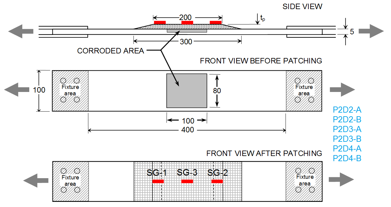
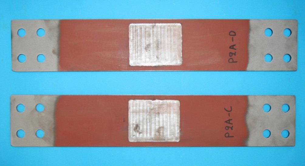
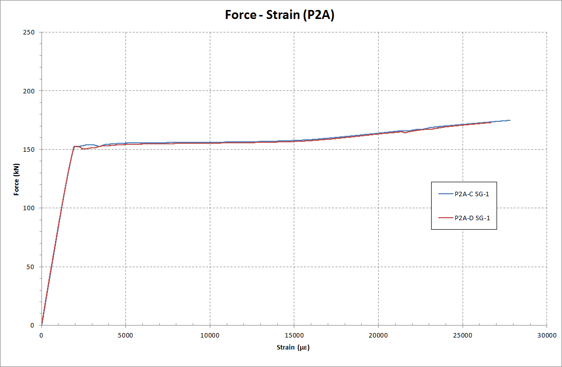
Figure 1.1: Example of a carbon fibre patch applied to a defected steel transverse frame. ............................. 2 Figure 1.2: Application of a composite patch on site (Grabovac et al, 2009). ................................................... 3 Figure 1.3: Patch with structural health monitoring system bonded to F-111 wing (Baker et al, 2009). ........... 4 Figure 1.4: Reinforcement of concrete bridge using carbon fibres. .................................................................. 5 Figure 1.5: Carbon fibre reinforcement and monitoring system in service (Grabovac et al, 2003). .................. 6 Figure 1.6: Composite patch configuration (Grabovac et al, 2009). 6 Figure 1.7: Photos depicting damage and the cut-outs made for welding a life raft support system on the deck (Grabovac et al, 2009). ............................................................................................................................. 7 Figure 1.8: Composite patch repairs on lift shafts of Type 42 destroyers. ........................................................ 7 Figure 1.9: Composite patch applied to cargo tank on-board FPSO (Turton et al 2005). ................................. 8 Figure 1.10: Repair on the corridor side of the Bulkhead (McGeorge et al, 2009). .......................................... 9 Figure 1.11: Glass fibre patching of sensitized aluminium deck. ...................................................................... 9 Figure 1.12: Cross-section of patch over sensitized aluminium plate. ............................................................ 10 Figure 1.13: Crack in aluminium superstructure and carbon / epoxy patch. 10 Figure 1.14: Area of damage (pictures a and b), lamination of the repair (c), finished coated repair (d). ...... 11 Figure 1.15: Position of cracks (a), treated surface (b) lamination of the repair (c), finished repair (d). ......... 12 Figure 1.16: Cross deck plating of a bulk carrier. ............................................................................................ 13 Figure 1.17: Defects in water ballast tank. ...................................................................................................... 13 Figure 1.18: Arrows pointing to fatigue cracks at bracket. .............................................................................. 14 Figure 1.19: General corrosion due to coating failure (left) and pitting corrosion (right). ................................ 14 Figure 1.20: Prefabricated pultruded carbon strips bonded onto a steel bridge. ............................................ 16 Figure 1.21: Curing of co-bonded patch. ......................................................................................................... 17 Figure 1.22: Types of failure in composite patch repairing (McGeorge et al, 2009). ...................................... 18 Figure 1.23: Skewed crack front in one sided repaired specimens (Lee and Lee, 2004). .............................. 20 Figure 1.24: Numerical model depicting debonding evolution (Papanikos et al, 2005). 21 Figure 1.25: Commercial wireless sensor nodes. ........................................................................................... 22 Figure 1.26: Optical Fibre system. ................................................................................................................... 22 Figure 1.27: Co-Patch project partners. .......................................................................................................... 24 Figure 2.1: Loading modes. 27 Figure 2.2: Stress field near a crack. ............................................................................................................... 27 Figure 2.3: J-Integral schematic. ..................................................................................................................... 29 Figure 2.4: Relative displacement at the crack flanks. .................................................................................... 30 Figure 2.5: The bilinear traction separation law. ............................................................................................. 36 Figure 2.6: MMB geometry parameters and test setup (Carlsson 2014). ....................................................... 37 Figure 2.7: Single leg bending tests performed by Lee et al (2010). .............................................................. 38 Figure 2.8: Partial adhesive failure of DCB specimens (Andersen 2005). ...................................................... 38 Figure 2.9: DCB-UBM test rigs. ....................................................................................................................... 39 Figure 3.1: P2 plates geometry. ...................................................................................................................... 41 Figure 3.2: Six P2D (2 painted and 4 unpainted) specimens after 75 days in the environmental chamber. .. 42 Figure 3.3: Fixture specimen assembly mounted for testing. .......................................................................... 44 Figure 3.4: Vacuum infusion setup (figure provided by AS2CON). ................................................................. 45 Figure 3.5: Manufacturing of P2D specimens’ patches (figure provided by AS2CON). .................................. 45 Figure 3.6: Instrumentation of specimens P2D1-A, P2D1-B, P2D3-B. ........................................................... 46 Figure 3.7: Instrumentation of P2D2, P2D3 and P2D4 specimens. ................................................................ 46 Figure 3.8: Thickness reduction of the central area of specimens P2A-C and D. 47 Figure 3.9: Force – Displacement curves of P2A specimens. ......................................................................... 48 Figure 3.10: Force – Strain curves (SG-1) of P2A-C and D specimens. ......................................................... 49 Figure 3.11: Specimen P2D2A being tested on MTS testing machine. .......................................................... 49

Vi

Figure 3.12: Qualitative Force – Displacement curves of P2D and P2-A specimens. .................................... 50 Figure 3.13: Yielding around the holes during testing. .................................................................................... 51 Figure 3.14: Force – Strain curves of P2D1-A specimen. ............................................................................... 51 Figure 3.15: Force – Strain curves of P2D2-A specimen. 52 Figure 3.16: Force – Strain curves of P2D3-B specimen. 52 Figure 3.17: Edge debonding of P2D specimens. ........................................................................................... 53 Figure 3.18: Bondline of the two coated aged specimens after testing. .......................................................... 54 Figure 3.19: Reduction of the effective bonding area due to corrosion in unpainted patched P2 specimens. 55 Figure 3.20: ¼ of the specimen that was modelled in ANSYS. ....................................................................... 56 Figure 3.21: Generated finite element model of the P2D1 plates. .................................................................. 57 Figure 3.22: Force displacement curve of the 3D finite element model .......................................................... 59 Figure 3.23: Plastic strain distribution at 147.00 kN. ....................................................................................... 59 Figure 3.24: Initiation (left) and development of debonding (right) in the 3D model. ...................................... 60 Figure 3.25: Experimental versus 3D numerical Force – Strain graph. 60 Figure 3.26: Deflection at 148.06kN (scale factor of 20). ................................................................................ 61 Figure 3.27: Generated 2D finite element model and mesh size .................................................................... 61 Figure 3.28: Force-displacement curves of the 2D and 3D numerical simulations. ........................................ 62 Figure 3.29: Force strain curves for the experimental and numerical results. ................................................ 63 Figure 3.30: Von Mises plastic strain at the steel substrate at 151.11 kN. ..................................................... 64 Figure 3.31: Comparison of FE models with different patch length to the experimental results. .................... 64 Figure 3.32: Force – Displacement curves of the undefected, corroded and repaired models. ..................... 65 Figure 3.33: Force-displacement of the intact, corroded, and repaired cases with different thickness diminution. ....................................................................................................................................................... 66 Figure 3.34: 2D FE patch model results for steel modelled with and without plasticity. ................................. 67 Figure 4.1: P1 plates geometry. ...................................................................................................................... 69 Figure 4.2: P1 specimen mounted on the testing machine. ............................................................................ 70 Figure 4.3: Instrumentation of specimens P1A-C and P1A-D. ........................................................................ 71 Figure 4.4: Instrumentation of P1D1-A, P1D1-B and P1D1-C specimens. 71 Figure 4.5: Instrumentation of P1D2-A and P1D2-B specimens. .................................................................... 72 Figure 4.6: Specimen P1D1-A being tested on MTS testing machine (left) and on INSTRON 300LX testing machine (right). ................................................................................................................................................ 73 Figure 4.7: Force – Strain curves of P1A-C and P1A-D specimens. .............................................................. 74 Figure 4.8: Force – Displacement (LVDT) curves of P1D1 specimens tested by NTUA. ............................... 75 Figure 4.9: Force – Displacement (Crosshead) curves of P1D specimens tested both by NTUA and AIMEN.

......................................................................................................................................................................... 76 Figure 4.10: Force – Strain curves of P1D1-A specimen’s first loading by NTUA. ......................................... 76 Figure 4.11: Force – Strain curves of P1D1-A specimen’s second loading by NTUA. ................................... 77 Figure 4.12: Force – Strain curves of P1D1-C specimen’s first loading by NTUA. 77 Figure 4.13: Force – Strain curves of P1D1-C specimen’s second loading by AIMEN. ................................. 78 Figure 4.14: Existing manufacturing flaw detected during non-destructive evaluation prior to testing. .......... 79 Figure 4.15: Markings denote the debonded/delaminated area after the final testing of specimens. ............. 80 Figure 4.16: Comparison of Force – Strain curves for P1D2-A and P1D2-B specimens. ............................... 80 Figure 4.17: Comparison of Force – Strain (SG-3) curves for all P1D specimens.......................................... 81 Figure 4.18: Acousto-ultrasonic inspection finding in specimens P1D2-A & B prior to testing. ...................... 81 Figure 4.19: Correlation of the outer surface markings to the bondline surface ............................................. 82 Figure 4.20: Schematic of specimen P1F ........................................................................................................ 84 Figure 4.21: Instrumentation of the P1F specimen. ........................................................................................ 85 Figure 4.22: Positioning of the optical fibres with the aid of laser pointers. .................................................... 86 Figure 4.23: Force - displacement curve of the reference and P1F specimen. .............................................. 87 Figure 4.24: Force-strain measurements of P1F specimen. ........................................................................... 87

Vii

Figure 4.25: Notch at the back side immediately before and after patch debonding. ..................................... 88 Figure 4.26: P1F specimen after testing.......................................................................................................... 88 Figure 4.27: Position of optical fibres OF1 (left) and OF-2 (right). .................................................................. 89 Figure 4.28: FE model of the ¼ of the specimen. ........................................................................................... 91 Figure 4.29: Force displacement curves. ........................................................................................................ 92 Figure 4.30: Debonding status at 157 kN. ....................................................................................................... 92 Figure 4.31: Von Mises stress distribution on the unreinforced side (left) and on the reinforced side (right) of the steel plate, at 157 kN. ................................................................................................................................ 93 Figure 4.32: Strain gage-1 measurements. ..................................................................................................... 93 Figure 4.33: Strain gage-2 measurements. 94 Figure 4.34: Optical fibre 3 measurements. .................................................................................................... 94 Figure 4.35: Optical fibre 4 measurements. 95 Figure 5.1: Geometry of P3 plates. .................................................................................................................. 97 Figure 5.2: Specimens’ manufacturing (Figure provided by AS2CON). .......................................................... 98 Figure 5.3: Example of needle gun scaler. ...................................................................................................... 99 Figure 5.4: Painted P3 specimens placed into the environmental chamber. ................................................ 101 Figure 5.5: Position of strain gages on P3 specimens. ................................................................................. 102 Figure 5.6: Instrumentation of specimens P3A-C, P3A-D, P3A-E, P3D1-A and P3D-B ............................... 102 Figure 5.7: Instrumentation of specimens P3D1-B and P3D4-A. 102 Figure 5.8: Instrumentation of specimens P3D2-A, B, P3D3-A, B, P3D5-A, B and P3D6-A, B. ................... 102 Figure 5.9: Definition of distances between notch tip and CG-1 and between CG-1 and CG-2. .................. 103 Figure 5.10: Both sides of specimen P3D4-B while tested in fatigue. ........................................................... 104 Figure 5.11: Indicative time strain measurements for specimen P3D1-A. .................................................... 106 Figure 5.12: α-N curves of the reference P3A specimens. ........................................................................... 107 Figure 5.13: α-N curves of P3D specimens. .................................................................................................. 107 Figure 5.14: Oblique crack propagation that resulted in fewer measurements by CG-2. ............................. 108 Figure 5.15: Findings of the initial NDE on the patch surface, for the grit blasted P3 specimens. ............... 109 Figure 5.16: Findings of the initial NDE on the patch surface, for the needle gun treated P3 specimens. ... 109 Figure 5.17: α-N curves of P3D specimens; comparison of surface preparation method. ............................ 110 Figure 5.18: Fatigue life N36-83 of all specimens. 110 Figure 5.19: α-N curves of P3D1 and P3D2 specimens................................................................................ 112 Figure 5.20: α-N curves of specimens P3D3, P3D4, P3D5 and P3D6-A. ..................................................... 113 Figure 5.21: Crack faces of two representative specimens........................................................................... 113 Figure 5.22: Initial non-destructive evaluation of the patch repair in P3D4-B (left) and evolution of debonding during fatigue testing (right). .......................................................................................................................... 114 Figure 5.23: Initial findings (a) projection of findings matching the dry area at the interface (b), dry plies detected by the inspection revealed after cutting the laminate (c). ............................................................... 115 Figure 5.24: Internal and external patch surfaces of P3 grit blasted specimens. The initial findings were marked on the external surfaces. 120 Figure 5.25: Internal and external patch surfaces of P3 needle gunned specimens. 121 Figure 5.26: Distinction between white and black areas on the internal surface of P3D5-B patch. .............. 122 Figure 5.27: Unpatched side of steel, showing the crack paths. ................................................................... 123 Figure 6.1: Aframax tanker depicting the modelled section. ......................................................................... 127 Figure 6.2: Bulkhead stiffeners modelled using shell elements (red) and Euler-Bernoulli beams (green). .. 128 Figure 6.3: Stiffeners’ mesh size. 128 Figure 6.4: Distribution of bending moment in the model after the adjustment. ............................................ 130 Figure 6.5: the FLD (top) and WBD (bottom) conditions ............................................................................... 131 Figure 6.6: Regions where the cracks were introduced. ............................................................................... 132 Figure 6.7: Derivation of the Uy displacement analytical field at the hopper floor boundary. ....................... 133

Viii

Figure 6.8: Distribution of the nodal rotations for the hopper floor boundary. ............................................... 134 Figure 6.9: Von Mises stress distribution near crack-1 for hogging (left) and sagging (right). ...................... 135 Figure 6.10: Distribution of stresses normal to crack-2 edges for hogging (left) and sagging (right)............ 135 Figure 6.11: Indicative figure showing the crack-2 edge penetration. ........................................................... 136 Figure 6.12: Crack propagation curve of AH36 steel along with the evaluated point for Crack-1................. 137 Figure 6.13: Cargo loading considered in the three compartment model. .................................................... 138 Figure 6.14: Displacement field along the Y (top) and Z (bottom) direction in the shell (left) and the solid (right) sub model. ........................................................................................................................................... 139 Figure 6.15: Crack locations. ......................................................................................................................... 140 Figure 6.16: Von Mises stress in the steel before (left) and after repair (right). ............................................ 143 Figure 6.17: Stress intensity factor across the thickness. ............................................................................. 143 Figure 6.18: Distribution of stress intensity factor in crack-2. ........................................................................ 145 Figure 6.19: One sided versus double sided patch configuration. ................................................................ 146 Figure 7.1: Representation of the CSDE method. ......................................................................................... 150 Figure 7.2: Illustration of the crack region of studied bimaterial interface. 151 Figure 7.3: Mesh size of the FE model for the implementation of the CSDE method. .................................. 152 Figure 7.4: Element arrangement and mesh density at the crack tip. 152 Figure 7.5: Extrapolation of the energy release rate. .................................................................................... 153 Figure 7.6: Extrapolation of the mode mixity. ................................................................................................ 154 Figure 7.7: Superposition technique (Suo 1990). .......................................................................................... 156 Figure 7.8: Moment equilibrium due to contact at the crack tip. .................................................................... 165 Figure 7.9: Axial force and moment equilibrium in a single strap joint. ......................................................... 166 Figure 7.10: Critical energy release rate models as a function of mode mixity. 170 Figure 7.11: Strain energy release rate and mode mixity versus thickness ratio (bending load).................. 171 Figure 7.12: Strain energy release rate and fracture toughness versus thickness ratio (bending load). ...... 172 Figure 7.13: Strain energy release rate and mode mixity versus bending stiffness ratio (bending load). .... 172 Figure 7.14: Strain energy release rate and fracture toughness versus bending stiffness ratio (bending load).

....................................................................................................................................................................... 173 Figure 7.15: Strain energy release rate and mode mixity versus thickness ratio (axial load). ...................... 173 Figure 7.16: Strain energy release rate and fracture toughness versus thickness ratio (axial load). ........... 174 Figure 7.17: Strain energy release rate and mode mixity versus axial stiffness ratio (axial load). ............... 174 Figure 7.18: Strain energy release rate and fracture toughness versus axial stiffness ratio (axial load). ..... 175 Figure 7.19: Strain energy release rate and mode mixity versus axial stiffness ratio (axial load) for the HLU ....................................................................................................................................................................... 176 Figure 7.20: Outline of repair assessment and decision making process (DNV-RP-C301). ......................... 178 Figure 7.21: Patch assessment and decision making procedure. ................................................................. 180 Figure 7.22: von Mises stress distribution (top) and longitudinal stresses (σz) in defected structure (bottom).

....................................................................................................................................................................... 182 Figure 7.23: von Mises stress distribution (top) and longitudinal stresses (σz) on the steel structure after the application of a HLU-CE patch. ..................................................................................................................... 183 Figure 7.24: von Mises stress distribution (top) and longitudinal stresses (σz) on the steel structure after the application of a VI-CE patch. ......................................................................................................................... 184 Figure 7.25: Stress distribution in the reinforced and unreinforced sides of the steel at the patch edge ..... 185 Figure A.1: Vacuum infusion of laminate (provided by AS2CON). ................................................................ 206 Figure A.2: Layer configuration used for each specimen type (provided by UM). ........................................ 206 Figure A.3: Plies configuration prior to infusion (provided by UM). ............................................................... 207 Figure A.4: Sealing and Vacuum Infusion of laminates (provided by UM). ................................................... 207 Figure A.5: Set-up of pre-preg prior to curing (provided by NTNU). ............................................................. 208 Figure A.6: PP-C/E-T-0 laminate after curing (provided by NTNU). 209

Ix

Figure A.7: PP-C/E-T-0 and PP-C/E-T-90 laminates with tabs prior to tab-adhesive curing (provided by NTNU). ........................................................................................................................................................... 209 Figure A.8: PP-C/E-T-0 and PP-C/E-T-90 laminates with tabs after tab-adhesive curing (provided by NTNU).

....................................................................................................................................................................... 210 Figure A.9: PP-C/E-S laminate after curing (provided by NTNU).................................................................. 210

Ist Of Tables

Table 3.1: Conditions of one accelerated corrosion cycle. .............................................................................. 41 Table 3.2: Nomenclature of P2 specimens...................................................................................................... 43 Table 3.3: Dimensions of P2 specimens. ........................................................................................................ 43 Table 3.4: Results of P2A specimens. ............................................................................................................. 48 Table 3.5: Patch Debonding Loads of P2D specimens. .................................................................................. 53 Table 3.6: Results of P2 plates. ....................................................................................................................... 56 Table 3.7: Average dimensions of the non-aged specimens. ......................................................................... 57 Table 3.8: Cohesive law properties. ................................................................................................................ 58 Table 4.1: Dimensions of P1 specimens. 69 Table 4.2: Nomenclature of P1 specimens...................................................................................................... 70 Table 4.3: Yield and maximum loads for P1 reference specimens. ................................................................ 74 Table 4.4: Results of P1D specimens. ............................................................................................................ 83 Table 4.5: Results of reference and P1F specimens. ..................................................................................... 88 Table 4.6: Patch material properties for the FE model of specimen P1F. ....................................................... 91 Table 5.1: Specimens’ geometry ..................................................................................................................... 98 Table 5.2: Surface preparation and aging scenarios of P3 specimens. ........................................................ 100 Table 5.3: Fatigue results of P3D specimens. ............................................................................................... 105 Table 5.4: Notch eccentricity measurements. 115 Table 5.5: Patch eccentricity measurements................................................................................................. 116 Table 5.6: Specimens characteristics measurements. 116 Table 5.7: Initial characteristics of patch or bond defects. ............................................................................ 117 Table 5.8: Patch quality classification ............................................................................................................ 118 Table 5.9: Comparison of repair characteristics and fatigue life. .................................................................. 124 Table 6.1: Principal characteristics of study case. ........................................................................................ 127 Table 6.2: Value of K and J for the WBD. ...................................................................................................... 136 Table 6.3: Calculated ΔK and crack growth rate ........................................................................................... 136 Table 6.4: Material properties of resin and steel. .......................................................................................... 140 Table 6.5: Patch dimensions. ........................................................................................................................ 141 Table 6.6: Studied cases. .............................................................................................................................. 142 Table 7.1: Crack tip convergence CSDE. 152 Table 7.2: Comparison of the CSDE to the enhanced VCCT and the J-integral. ......................................... 155 Table 7.3: Extraction of ω values for different cases ..................................................................................... 160 Table 7.5: ω values table for the reduced formulation. ................................................................................. 162 Table 7.6: ω values table for the full formulation. 163 Table 7.7: Results for bending moments with different signs. ....................................................................... 166 Table 7.8: Edge versus crack debonding in cracked cases. 167 Table 7.9: Cases of the parametric study. ..................................................................................................... 169 Table A.1: Experimentally measured material properties. ............................................................................. 211 Table A.2: Engineering Constants. 211

Ntroduction

The various structural parts and details of a steel ship are subjected to a plethora of loading conditions during the vessel’s operational life. The type and magnitude of these loading conditions vary significantly due to the stochastic nature of sea waves, which are the major cause for the loading applied to a marine structure. For this reason, it is quite usual to notice various types of local defects and failures in a ship structure, like plastic deformations and development of cracks, not forgetting corrosion, which increases the susceptibility of the structure to such local defects. In particular, in the presence of stress concentrations, fatigue loads acting on the structure can generate cracks, which, if not detected and repaired in time, can grow up to a critical length and cause catastrophic failures. Another typical defect of marine structures is corrosion that reduces the plate thickness, causing deterioration of the stiffness of the metal structure.

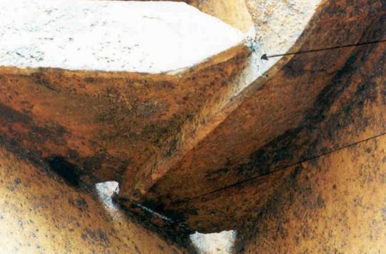
Nowadays the tendency to use high strength steel and the consequent reduction of plate thickness accentuates the problems generated by corrosion. Thus, there are many cases in a steel marine structure where the need arises for local reinforcements or repairs, either permanent or temporary, until the next programmed inspection and maintenance. This need can also be the consequence of requirements for higher load-carrying capacity of the structure, which can in turn be the result of either a problematic initial design (i.e. existence of high stress concentrations which were not initially predicted) or an improper manufacturing or erection procedure, or a change in the operational conditions (i.e. later additional loading).

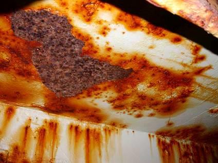
Another very common reason for local repairs is the existence of defects in the steel structure resulting from accidents or overloading. The basic objective of these local reinforcements and/or repairs is the increase of the structure’s residual strength in static loading or the elongation of its operational life in cyclic loading.

Composite material patching is a very promising new method for repairing and/or reinforcing steel structures. The technique consists of the application of a patch made of fibrous composite materials on the metal structure to repair or improve static strength (Figure 1.1). The patch is effective due to the fact that part of the applied load acting on the patched structure is transferred from the base metal plate through an adhesive layer to the composite patch, thus reducing the stress levels in the metal substrate under the patch.

Thus, in the case of cracked structures, a composite patch decreases the stresses in the area of the crack tip therefore decelerating or under certain conditions completely arresting the crack. If the damage of a marine structure is not too severe or if the need for improvement is small, the structures are generally repaired or reinforced through the addition of plates (the so-called doubling) or stiffeners by means of welded or bolted joints, or by welding-in the cracks in the case of cracked structural members. In the case of most severe conditions (for example when the damage is widespread over a large part of the structure), the replacement of the whole portion of the structure is necessary. The use of these traditional methods offers several advantages to all stakeholders involved in ship repair/reinforcement business (ship-owners, shipyards, Classification Societies, Authority Flags, etc.). The advantages are essential due to the fact that being a well tried and trusted practice, the designers do not have excessive difficulties to design the repair/reinforcement, because the use of welded and bolted joints has been widely discussed in many literature papers and is also included in many Rules and Regulations. Furthermore, the Classification Societies usually accept these solutions without further investigations or analyses beyond those already foreseen from standards or regulations. In addition, the availability of qualified personnel able to deal with these methods encourages their use for repair and/or reinforcement. However, welding and bolted joints repair/reinforcement methods have also several disadvantages that in some circumstances make these techniques costly and time-consuming or simply impossible to be used.

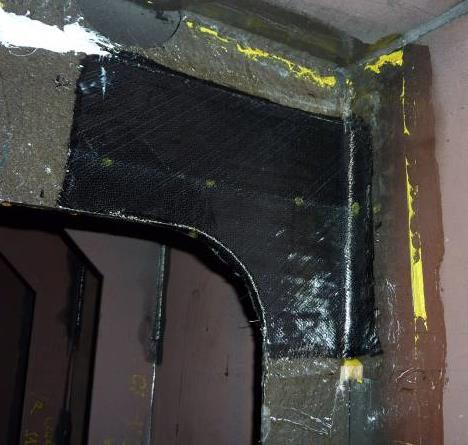
Figure 1.1: Example of a carbon fibre patch applied to a defected steel transverse frame. First of all welding in explosive environment (e.g. in the double bottom of a fuel oil tanker) requires a very complicated and expensive preparation procedure and the repair/reinforcement can be executed only under rigorous safety precautions; furthermore, traditional repair techniques often require the availability of complicated and costly infrastructures (dry-docks, cranes, scaffolding, etc.) and the application of an either welded or bolted joint, if not carefully designed, can generate new stress concentrations that mitigate the effect of the repair/reinforcement. Also the addition of weight caused by the application of welded or bolted doubler plates is a significant drawback that the designer should keep into account in order to avoid excessive weight increase. Another disadvantage, is that welding methods are not directly applicable on structures subject to significant loads (i.e. by their own weight), because welding generates high temperatures that can cause catastrophic collapse of the structures under tension. All the above mentioned drawbacks have negative effect on the cost of the repair/reinforcement, since the ship may stay out of operation for a relatively long period; thus, investigating new solutions alternative to welded and bolted joints can help improve the repair/reinforcement process. From this point of view, the use of composite materials patches appears to be a very promising way to repair/reinforce metal structures, because it overcomes most of the above mentioned drawbacks of the traditional techniques.

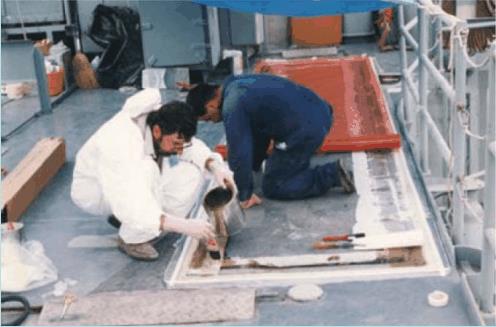
Applying a composite patch requires neither hot-work (so they can be used also in explosive environments or in structures subject to significant loads), nor the presence of special infrastructures since the patches are directly applied to the metal with a simple preparation of the surface. Composite patches can be quickly applied with no geometric or shape restrictions in their application. Furthermore the added weight is very limited. For these reasons the patches can be usually applied ‘in situ’ while the structure is in service (Figure 1.2). In addition, contrary to the welded or bolted joints, composite patches do not generate stress concentrations on the repaired/reinforced structures.

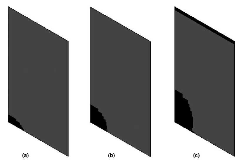
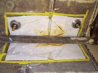
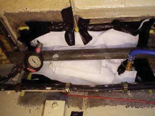
Figure 1.2: Application of a composite patch on site (Grabovac et al, 2009). Regarding the consequences on the environment and on the climate change, the use of composite patches is not considered to have negative effects. On the contrary, the reduction of downtime for ships or civil structures has positive effects, as there is no need any more to perform many and lengthy traditional repair works; also the minimization of traffic disruption reduces the traffic congestion and therefore positively affects the environment. Since the quantities of material used to fabricate the patches are quite small and the composite recycling technologies are making significant progress, it is possible to state that the influence on the environment is negligible.

All the above mentioned advantages make composite patches a new interesting method that, in several cases, can substitute the techniques involving welded and bolted joints and allows the reduction of the time and cost of the repair/reinforcement of the metal structure.

However, there are some parameters regarding the use of composite patches as a repairing/reinforcing technique that require additional investigation and studies. The most critical aspect concerns the long-term performance of the steel-adhesive-composite system, because it is subjected to the influence of complex external environmental parameters that makes it difficult to predict the behaviour of the patched structure in the long-term period. So far the topic has not been investigated in a satisfying way in the marine field, while the problem has already been widely investigated in the aerospace sector, where nowadays the use of patches is a common and trusted practice.

Applications Of Composite Patch Repairs

As mentioned earlier, composite patch repairing originates from the aerospace industry where boron/epoxy patches have been used to arrest fatigue cracks in the wings and fuselage of military aircrafts since the 90s (Figure 1.3). The first applications of such repairs have been performed by the Royal Australian Air Force (Molent 1989, Baker 1984) with Baker, Rose and Jones being among the pioneers in this field, focusing on the design, monitoring and environmental or operational effects on repaired aluminium structures (Baker et al 1984, 1988, 1999, 2004, 2009). Katnam et al (2013) provided an extensive literature review of patch repairing of composite structures on the aerospace field.

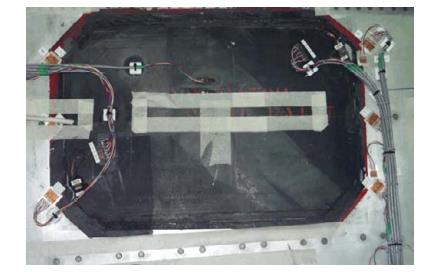
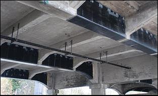
Figure 1.3: Patch with structural health monitoring system bonded to F-111 wing (Baker et al, 2009). In the civil sector composites have been recently utilized for strengthening or repairing beams, slabs and bridge decks (Figure 1.4) and a limited number of application cases have been reported, mainly in the UK. In civil engineering, bridges might be constructed using reinforced concrete, cast iron, wrought iron, steel and even masonry, as, unlike aerospace and marine applications, bridges are designed with a significantly larger operational life. In fact a recent survey on the age profile and condition of existing European bridges revealed that around 35% from a sample of 220000 bridges were over 100 years old (Larsen et al 2010).

Bearing this in mind, it is obvious that these structures were considered according to outdated techniques and materials and in order to remain in service they need to be strengthened to accommodate bigger loads or to mitigate the effects of defects and outdated design and construction practices. A review on the application of fibre reinforced plastics with an emphasis on metallic bridges can be found in Hollaway (2013), while Zhao and Zhang (2007) provided a state of the art of current research on FRP strengthened steel structures focusing on the strengthening of steel hollow section members and fatigue crack propagation in Figure 1.4: Reinforcement of concrete bridge using carbon fibres.

It would be expected that the technology associated with the bonding of composite materials to different substrates has matured and the experience gained primarily from the aerospace sector would make it easy to implement it also in the marine and offshore structures. This expectation is partially true as, indeed, the potential has been proven in praxis and data of their long term performance are available, but still there are several fundamental differences between the aerospace applications and marine/offshore steel applications which dictate a different approach and further investigation. These differences include the different stiffness of the base metal (stiffer steel versus the more similar to composites flexible aluminium), the completely different geometries involved (significantly thicker plating and larger beams in steel structures), the different loading cases and the different operating and environmental conditions. Furthermore, the operating time is greater for marine structures which in conjunction with their increased complexity and sparser inspection raise questions relatively to the long time performance of such repairs. Last but not least, the regulatory framework related to marine structures is more intricate as flag state regulations, classification societies’ requirements and national and international authorities are involved.

In the marine sector, there have been only a handful of documented applications and, as with the aerospace sector, most of them have been performed in military vessels. A first perspective for the development of the composite patch repair technology and its application in big ships was given by Grabovac et al (1993, 1997, 1999, 2003, 2009). In these works a brief description of the developments of the composite patch repair technology in the marine sector is given and an application case is presented in detail, including analysis of the superstructure cracking problem, research and development work, installation of composite reinforcement on board the ship, assessment of reinforcement efficiency, through-life monitoring and maintenance and repair. The application consists of repairing the aluminium deckhouse of a Royal Navy frigate that repeatedly exhibited fatigue cracking (Figure 1.5). The preferable installation procedure according to the authors is to grind out the crack and re-weld, then grind out the weld flat and affix the patch.

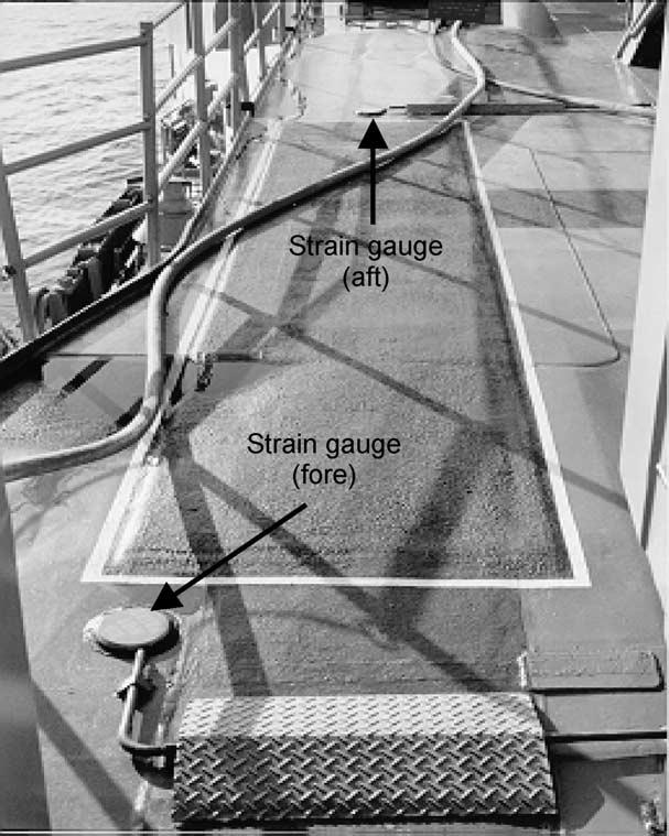
Figure 1.5: Carbon fibre reinforcement and monitoring system in service (Grabovac et al, 2003). During the vessel’s service period, seven inspections were made using non-destructive evaluation techniques combined with visual and acoustic tests. A total of four repairs were made during the 15 years of service. One repair was a non-structural restoration involving only the sacrificial edges of the GRP protective layers. The other three interventions were all structural repairs. Of those, two can be classified as dockyard inflicted damage that occurred during the ship maintenance or upgrade activities. The other may be regarded as environment initiated damage affecting the bonding at the overlay/deck interface which went unnoticed over a length of time. That was because the marine system paint failed to provide adequate protection to water ingress at the composite metal interface, and a new approach using an edge sealant was used (Figure 1.6). Additionally a time-cost estimation is given for the repairs. Apart from the repairs, the patch was cut in some locations so as to weld a support frame for the installation of a life raft (Figure 1.7). Although the welding operations were carried out in close proximity to the patch, no visible damage was noted. The installation of composite patches in stress concentration areas where the fatigue crack initiated in the past, led to a 20% reduction of stresses and after 15 years of active service no cracking underneath the patch or in adjacent areas was initiated.

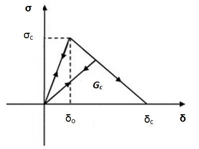
Figure 1.6: Composite patch configuration (Grabovac et al, 2009). Figure 1.7: Photos depicting damage and the cut-outs made for welding a life raft support system on the deck (Grabovac et al, 2009).

Dalzel-Job et al (2003) reference the applications that existed by that time, starting from the composite repairs in the aluminium superstructures of some frigates of the UK Navy performed in the 80s. The same work presents also the results of a corresponding experimental program, where thick (15 mm) steel plates with a central crack were reinforced with carbon/epoxy patches and then subjected to fatigue loading (σ = ± 100 ΜPa). The patch survived without any problem more than 1000000 loading cycles, equivalent to 12 ship years which was defined as the limit. The fatigue life of the plate was extended by at least 3 times, by applying the patch. In a subsequent work (QinetiQ, 2004), reference is made to the cases where the composite patch repair technology can or has already been applied in both marine (Figure 1.8) and aviation sectors, highlighting its advantages against traditional methods of repair. A brief description of the health monitoring systems applied in composite patch repairs is also presented. An important remark stated is that better and longer-term repairs are often achieved by laying up the patches and curing them in a continuous operation rather than bonding a pre-manufactured patch to the affected structure.

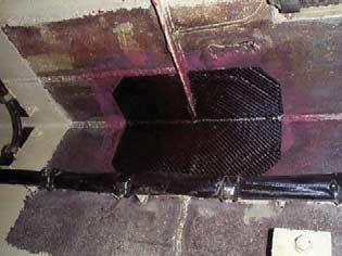
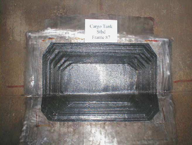
Figure 1.8: Composite patch repairs on lift shafts of Type 42 destroyers. In the work by Turton et al (2005) a description of the major advantages of this technology against the conventional repair methods is given followed by a brief description of case studies that took place from 1982-2003 in two different types of frigates and a FPSO unit (Figure 1.9). In all aforementioned cases composite patches were installed to arrest the propagation as well as the initiation of fatigue cracks. A qualitative comparative study between three methods for manufacturing the patches namely hand-lay-up, vacuum–infusion and pre-preg is presented. Additional experimental research performed in the same scope showed that composite patch application can increase the fatigue life of a cracked steel plate by a factor of over three times and that a patch has survived fatigue cycling equivalent to at least 12 ship years with no sign of patch delamination. Additionally, four different ultrasonic inspection techniques where examined for the non-destructive evaluation (NDE) of the repair with manual pulse echo contact ultrasonics and tandem pulse-echo ultrasonics being more promising at checking the quality and effectiveness of a composite patch.

The alternating current potential difference (ACPD) technique was used for monitoring the crack growth on two field applications on frigates. Figure 1.9: Composite patch applied to cargo tank on-board FPSO (Turton et al 2005).

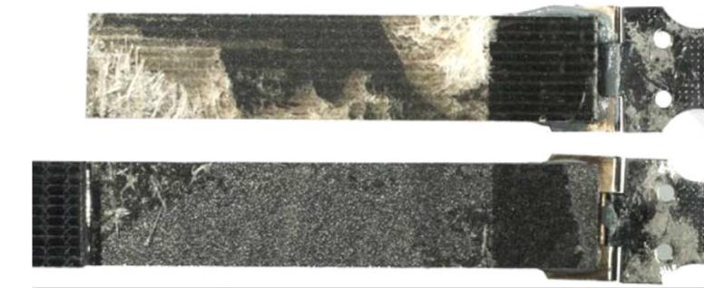
Another more recent work dealing with the application of composite patch repairs in marine structures is that of McGeorge et al (2009) where a procedure for the design and qualification of bonded repairs of floating offshore units used in the oil and gas industry has been developed. The use of this procedure has been demonstrated by two full-scale repairs that were carried out in two different FPSO units. The first repair was carried out in order to arrest a fatigue crack that had developed from the corner of a door (Figure 1.10), while the second one was carried out to restore material loss on a heavily pitted deck floor. The procedure is based on the use of relatively simple design methodologies that are derived from fracture mechanics theory.

The two demonstrators have shown the viability of bonded composite repairs to the two most widely encountered damage scenarios in floating offshore units – fatigue cracking and patch thinning due to corrosion.

Figure 1.10: Repair on the corridor side of the Bulkhead (McGeorge et al, 2009). The U.S. Naval Warfare Centre, Carderock Division, have used composite patches to cover large areas of sensitized aluminium plate on the superstructure of ships. For unknown reasons, but possibly due to changes in the processing by the aluminium mill, several U.S. Navy ships have suffered sensitization of 5456-H116 aluminium plating. Sensitization is a process where over time with exposure to higher service temperatures the magnesium that had been disbursed throughout the grain structure of the aluminium migrates to the grain boundaries, causing stress-corrosion cracking. Because the sensitization occurs throughout the aluminium plate, weld repairs to cracks are not effective because the plate adjacent to the weld, which is sensitized, will crack from the residual stress of welding. The only solution to the problem appeared to be total replacement of the plating, which would be extremely costly.

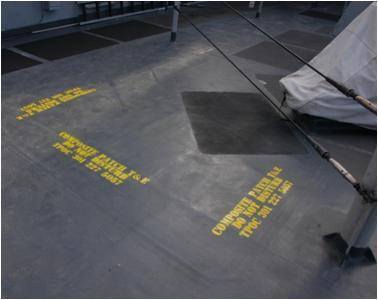
To address the problem and, at a minimum, provide watertight integrity, a repair procedure using low- elastic modulus E-fibre glass was used, laying down patches over large areas of the structure, as shown in Figure 1.11. The patches were designed to be of low stiffness so as to not attract more stress in the area that could cause cracking beyond the boundary of the patches. However, it is intended that the patches will reduce the stress intensity at the tips of the cracks under the patches, reducing the rate of fatigue crack propagation.

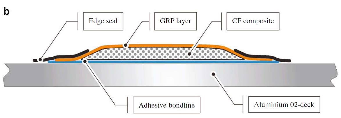
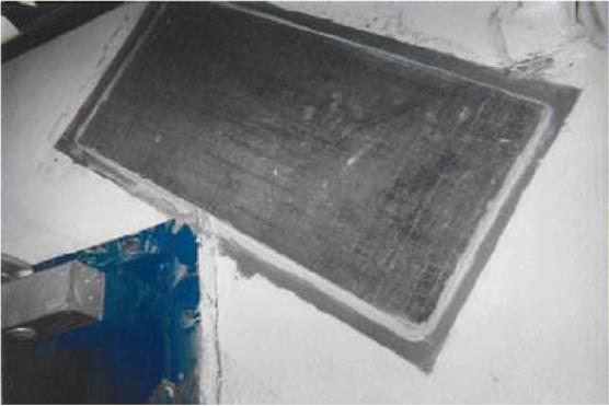
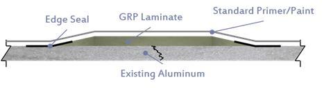
Figure 1.11: Glass fibre patching of sensitized aluminium deck. A cross-section through the patch is shown in Figure 1.12. Prior to patching, the surface was prepared by disk grinding. Subsequently it was cleaned using a solvent and a coupling agent was applied. The patch area was vacuum bagged and cured at 60ºC (140ºF) for eight hours. An epoxy system that would permit curing at a lower temperature was selected to prevent further sensitization of the plate. The edges were sealed with polysulfide to prevent water egress to the patch, taped over to prevent damage from abrasion, and then the entire area was painted over and marked as shown in Figure 1.11 to reduce the risk of inadvertent damage to the patch. The above work was carried out on several ships to cover a total area of about 100 sq. meters.

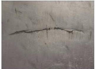
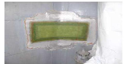
Figure 1.12: Cross-section of patch over sensitized aluminium plate. The French Navy has used composite patches to repair and prevent cracking in the aluminium superstructure of naval ships. Carbon fibre patches with an epoxy matrix were applied over cracks as shown in Figure 1.13. Temporary shelters were placed around the work area to control the environment. The laminate was vacuum-bagged and cured at 100ºC for two hours. These composite patches are expected to extend the service life of the ships by 20 years. The selected application method was grinding of the surface, followed by the application of a primer.

Figure 1.13: Crack in aluminium superstructure and carbon / epoxy patch. opportunity to apply composite patch repairing in the field in different applications. Two of them are presented here. The first one consisted of rehabilitating a corroded part at the fore ballast tank of a LPG tanker with a DWT of 9130 t. In particular, due to extensive pitting corrosion a hole was created in the bulkhead separating the ballast tank from the adjacent deep fuel tank. This led to loss of impermeability and therefore to the mixing of water ballast in the fuel tank and to the contamination of water ballast with fuel oil.

The latter was by far more critical as it led to the discharging of fuel oil to the sea each time the ballast tank was emptied, which is a severe violation of the existing regulations. A rotating wire brush has been used for the surface preparation of the area prior to lamination and the achieved roughness was on average Rz = 45 μm. The steel and ambient temperature was 31oC and 28oC respectively. The patch consisted of 16 layers of 200 g/m2 biaxial carbon reinforcement impregnated in epoxy resin in which an additive (KONASIL K-200) has been added to control the viscosity of the resin. A biaxial glass layer has been laminated between the steel plate and the patch to act as an isolating layer and prevent galvanic corrosion of the steel. The patch was laminated using the hand lay-up technique and the repair was successfully completed the same day.

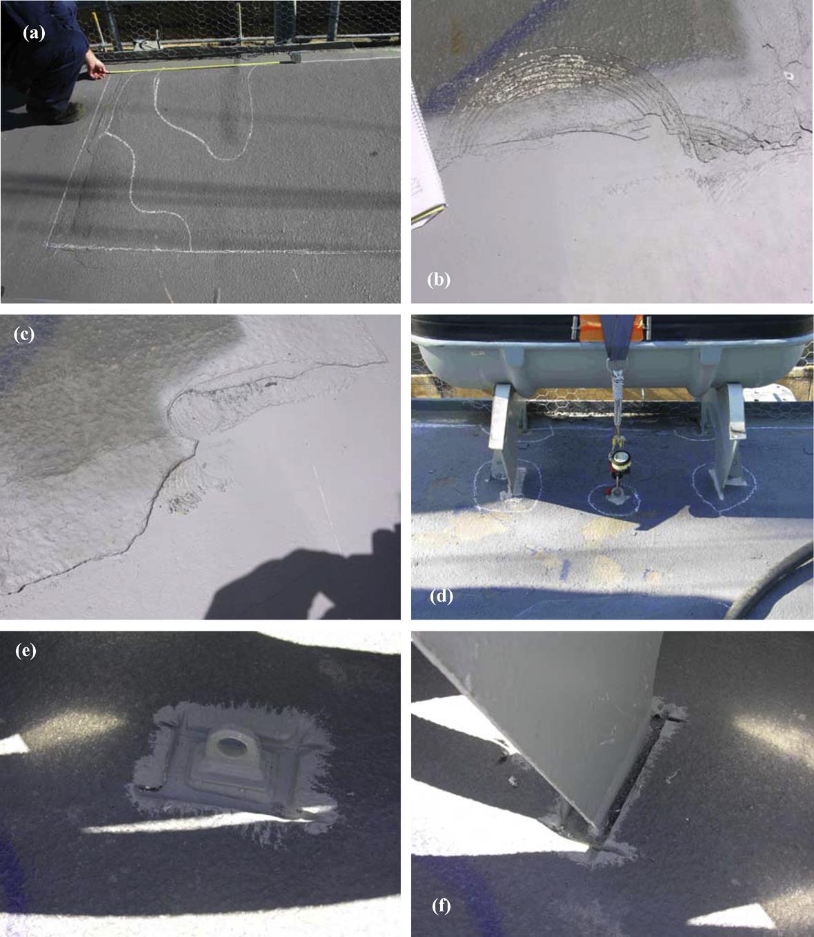
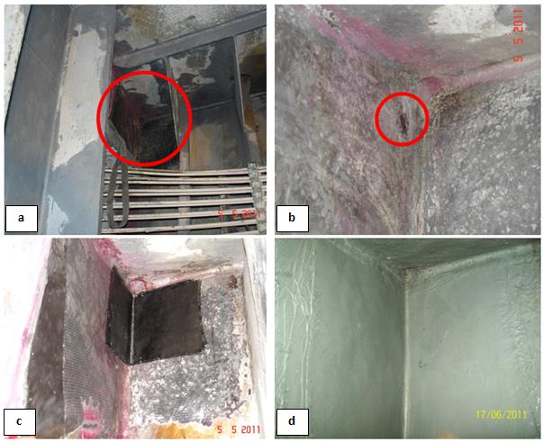
After curing, a typical marine coating has been applied in the area (Figure 1.14). The repair has been in service for four years with no reported reoccurrence of the problem and no visible signs of damage in the patch.

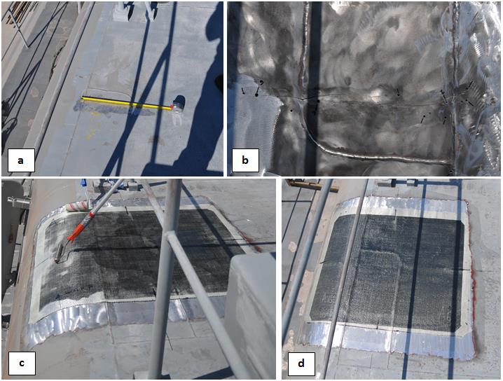
The second application case was performed in a vessel of the Hellenic Navy. A cluster of cracks was detected in the aluminium deck plating of one of the vessels as depicted in Figure 1.15. The cracks were formed due to unsuccessful attempts to repair the initial crack by welding, which eventually resulted to the formation of new cracks in the vicinity of the initial one. A carbon fibre patch with epoxy matrix was applied to repair the defects. Holes were drilled at the crack tips to act as crack arrestors and the aluminium surface was grinded using a rotating wire brush and cleaned with the use of a solvent. The first ply consisted of a glass layer to prevent galvanic corrosion between the carbon patch and the metallic substrate. The patch lamination was successfully completed the same day and left to cure at ambient conditions (around 40oC).

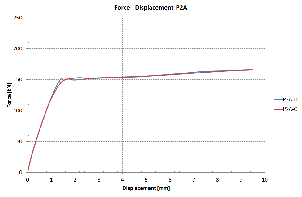
Figure 1.14: Area of damage (pictures a and b), lamination of the repair (c), finished coated repair (d). Figure 1.15: Position of cracks (a), treated surface (b) lamination of the repair (c), finished repair (d).

Ain Types Of Damage In Marine Structures

Ship and offshore structures will invariably face structural damage throughout their operational life. In this section, some of the most common, non-accidental structural defects are listed, in an attempt to identify possible patch repair application cases (Larsen et al 2010). The list is focused on typical known defects found on-board bulk carriers, oil tankers and containerships but not necessarily limited to these, as similar defects are prone to appear in other types of ships.

Reinforcement Of Cross Deck Plating

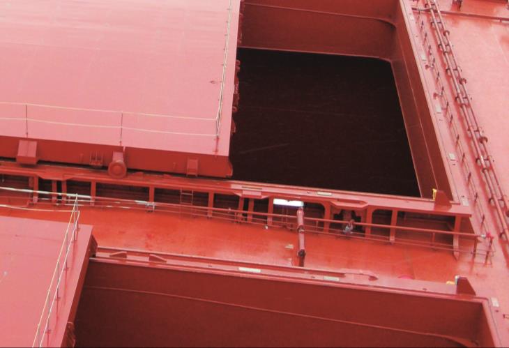
In the case of bulk carriers, due to the large open areas produced by cargo hatchways, the main deck which is a primary longitudinal strength component is continuous only at the outer strakes of the deck (Figure 1.16). This dictates that the cross deck plating experiences high loads to compensate for the discontinuity of the deck structure which can result in the buckling of the cross deck plating. This might be the result of sea loads acting directly on it, excessive loading in two adjacent holds, insufficient transverse stiffening or thickness diminution due to corrosion or a combination of the aforementioned. In the case of containerships, buckling might also be caused by the torsional deflection of the ship, as this type of ships are susceptible to torsional loads due to the big hold openings compared to bulk carriers.

Figure 1.16: Cross deck plating of a bulk carrier.

Reinforcement In Way Of Structural Details

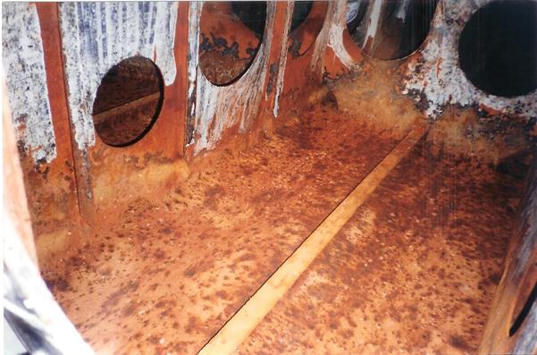
These types of damage involve typical defects located in way of lightening holes, girders, swash bulkheads and openings such as cut outs designed to allow the passage of stiffeners and other structural components (Figure 1.17). These areas typically introduce stress concentration points and, in combination with high loading and/or aggressive environment and the topology of the area, are prone to fracture, cracks, excessive deformation, corrosion and buckling.

Figure 1.17: Defects in water ballast tank.

Efects At Bracket Edges And Bilge Hopper Plates

Fractures may appear in details such as brackets. It is envisaged that the complex arrangement of some components may render these difficult to access. Cracks or fractures may occur at the connection of the bilge hopper plate and web frames in oil tankers due to stress concentrations along with static and dynamic loads from fluids (Figure 1.18).

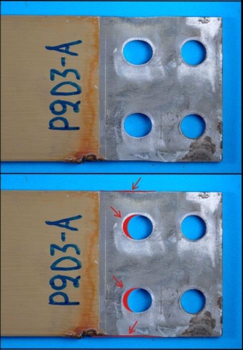
Figure 1.18: Arrows pointing to fatigue cracks at bracket.

Orrosion

Corrosion can occur for various reasons including lack of maintenance, interaction of cargo ingredients with steel, unintentional sacrificial protection (such as the hull becoming an anode in the process), stress corrosion or erosion. This application case concerns general and pitting corrosion (Figure 1.19) and it is essential that the cause of the corrosion is determined prior to treatment. Where general or pitting corrosion exists, if the thickness reduction is not significant then blasting of the surface and the application of a new coating is sufficient. In the opposite scenario, rectification measures must be sought. In all cases the Classification Society apply rules which specify acceptable diminution limits of the steel and this must also be considered prior to application of patches in this case. The allowable diminution of a component is usually given as a percentage of the as-fitted thickness of the component, while for pitting corrosion the acceptable diminution is based on a combination of pitting depth (referred to as intensity) and the surface area of the affected steel.

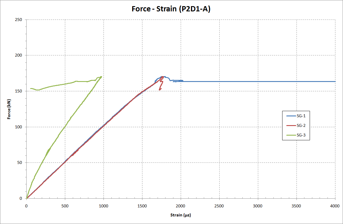
Figure 1.19: General corrosion due to coating failure (left) and pitting corrosion (right).

Fabrication Methods Of Patches

The joining of dissimilar materials has become a growing research area, as these joints are generally the weakest part of hybrid structures. The most common types of joining methods in composite structures are mechanical joining and bonding. Mechanical fastening rely on mechanical means such as rivets or bolts, which in most cases require drilling holes. Although this method makes the disassembly and the inspection easier, it also leads to undesirable stress concentrations, increase of weight of the structure and non-uniform load transfer through the joint. On the contrary, adhesive joints provide a more uniform load transfer and do not add to the weight of the structure, while rivets or bolts, where stress concentrations appear, are not required. Moreover, it is an ideal method for joining different materials, especially composite materials to metallic ones. For these reasons, adhesively bonded joints are increasingly being utilized substituting traditional methods of bonding such as welding, fastening and bolting. On the other hand, adhesive bonding is sensitive to environmental conditions, both during manufacturing and in service, and the appropriate surface treatment, which depends on the type of the adherents, is crucial for the good performance of the joint. In fact, surface treatment is considered as the weakest link in adhesively bonded structures and it is of paramount importance for the success and efficiency of the repair (Davis et al 1999).

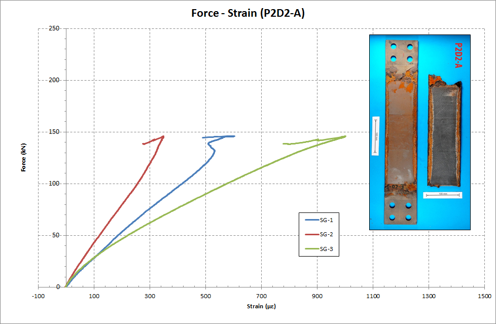
Surface preparation includes the cleaning of the substrates from any kind of contaminants such as rust, oil, grease, dust etc. that are detrimental to the bond. At the same time several studies have showed that increasing the surface roughness leads to the enhanced performance of the bond, as a certain degree of mechanical interlocking between the adhesive and the substrate is achieved. This interlocking is connected to the achieved surface roughness of the surfaces of the adherents and can be achieved either by mechanical or by chemical methods. Since immersion of the substrates into a chemical solution is inevitable when using a chemical treatment method, it is impractical to apply such a method to the large scale structures incorporated in the marine industry. In the framework of mechanical treatment methods, polishing, grit blasting and the use of power tools such as rotating wire brushes or emery cloth are the most common techniques utilized for roughening the adherents’ surfaces. These techniques depend on the type of the substrate, with grit-blasting being applied on metallic surfaces of metal adherents while polishing is applied to the composite ones. Comparative studies between different mechanical and chemical surface preparation for adhesive bonding have been performed by Siddaramaiah et al (1998) Grabovac et al (2003, 2009), Dag McGeorge et al (2009), Liu et al (2009), Andersen (2006) and Tsouvalis et al (2008). In each case, results indicated that grit-blasting led to better results.

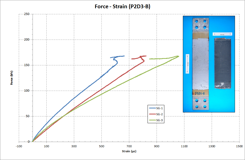
Composite patches can be divided in two main categories in terms of the installation method. The first category consists of composite patches that are prefabricated and subsequently transferred and bonded in the defected structure with the use of specialized adhesives. The second approach consists of in situ lamination of the composite patch directly on the structure and curing it on site. In this case, the matrix of the composite acts as the adhesive upon curing. Each method presents advantages and disadvantages and which one is more favorable depends on the application at hand. The two methods are described below.

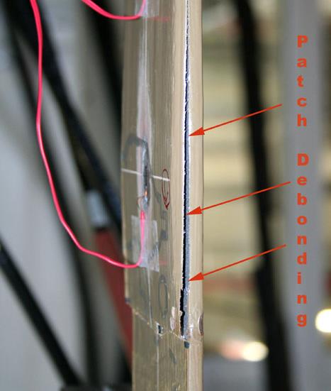
Adhesively Bonded Patches

This approach presents the advantage that a high quality composite laminate can be achieved as the employment of greater range of manufacturing techniques, spanning from the simple hand lay-up technique to more advanced methods such as prepregs, pultrusion and injection moulding. Additionally, the curing cycle can be better controlled and the risk of contamination or inappropriate curing of the laminate is significantly lower compared to the in situ lamination. Another advantage is that the designer is able to choose from a wide variety of specialized industrial adhesives to better suit the needs of each application.

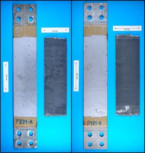
On the other hand, the procedure becomes more complicated as the correct application of the adhesive becomes crucial and suitable surface preparation of the composite material is necessary to ensure that adequate bonding is achieved between the patch and the selected adhesive. In addition, prefabricated patches are less versatile in terms of transportation, especially when the damaged area is hard to access or if the geometry of the member to be repaired is complicated. Another challenge is associated with the thickness and quality of the adhesive layer. Studies have been presenting contradicting results on the effect of the adhesive thickness with some claiming that a thick adhesive layer is desired (Mall 1989, Kawashita 2008) and others that an increased adhesive thickness is detrimental (Grant et al 2009, Tamblin et al 2001).

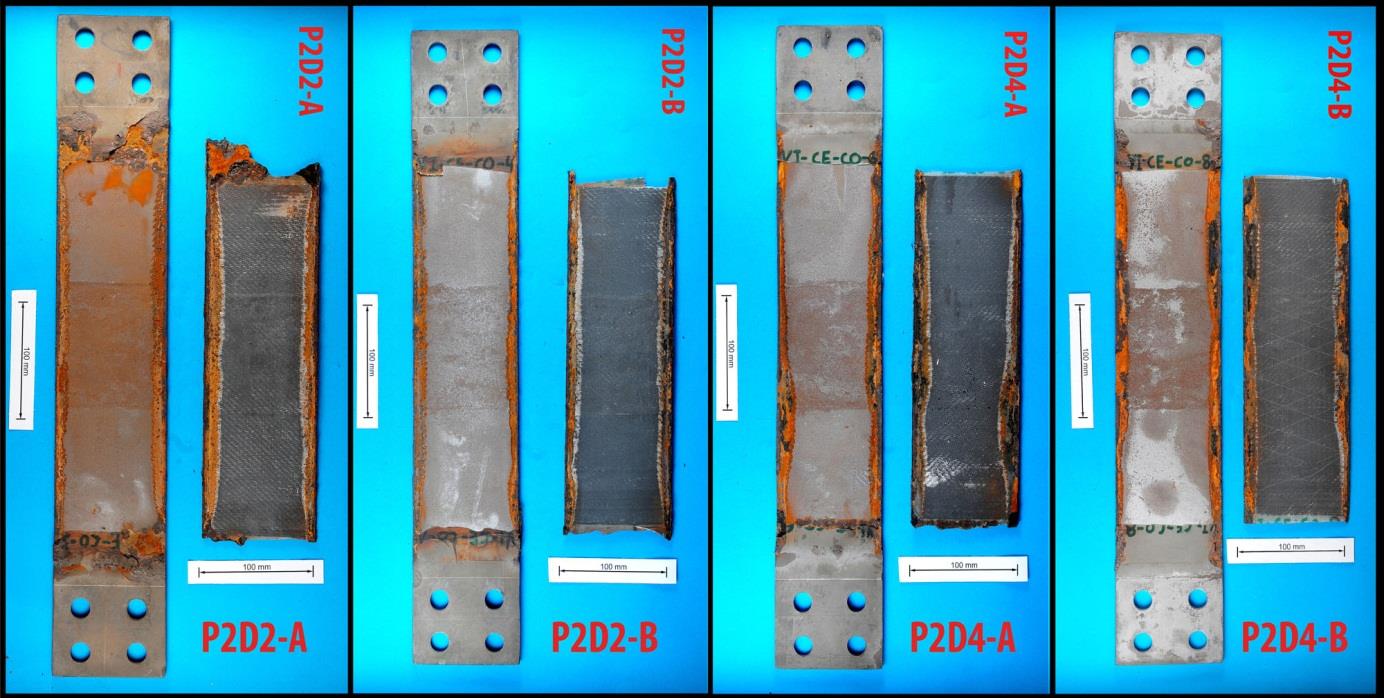
In reality a relatively thick adhesive is susceptible to imperfections caused from voids that might lead to premature failure and in practice, controlling the adhesive thickness and achieving a uniform thickness has proven to be challenging, even more so in cases where the base material surface is uneven. Additionally, the challenge of properly curing the adhesive is not surpassed, if not increased, as the bulk of the material between the substrates is not accessible. This method nevertheless has been used in civil engineering, especially by using pultruded or prepreged unidirectional beams or tapes that are subsequently bonded to bridge deck and girders. Such an application case is illustrated in Figure 1.20.

Figure 1.20: Prefabricated pultruded carbon strips bonded onto a steel bridge.

O-Cured Bonded Patches

In situ curing or alternatively co-cured bonding use the excess resin of the composite system during the curing process as the adhesive, forming bondlines with thicknesses typically less than 0.1 mm. This method presents several advantages compared to adhesively bonded joints where a different adhesive is used, as the design, analysis and manufacturing of these kind of joints is simpler compared to adhesive joints, it requires no surface preparation of the composite adherent and it is considerably faster, as the bonding process is performed simultaneously to the curing process of the composite system. Despite the practicality of this method, only a few studies on co-cured bonding are available studying the behaviour of single lap and double lap joints under static and fatigue loading (Shin et al 2003, 2006, Park et al 2006, Russo 2011, Song 2010).

The drawbacks associated with this method are that the manufacturing procedures that can be applied on site are limited mainly to hand lay-up, vacuum bagging and vacuum infusion and careful planning and execution has to be followed in order for them to be successful. Moreover, additional preparation might be necessary to control the ambient conditions on site and mitigate detrimental environmental effects that can lower the efficiency and the life expectance of the repair. Such measures involve the isolation of the area and position of heaters and dehumidifiers if it is in an enclosed space. Concerning the curing cycles, these can be achieved in a satisfactory way by the use of heating blankets, specialized portable curing devices (Figure 1.21) or even heat induction curing in the case of carbon fibres (Grabovac 2009). It is deemed that this bonding technique is better suited for marine applications, as defects in marine structures tend to be located in areas where the topological features of the structure change and access could be limited, especially if these are located inside holds, tanks or at the double bottom of the ships’ structure. Additionally, especially in the case of corrosion, the area to be repaired might be considerably large rendering the use of prefabricated patches logistically complicated and more cumbersome (QinetiQ 2004, McGeorge et al 2009).

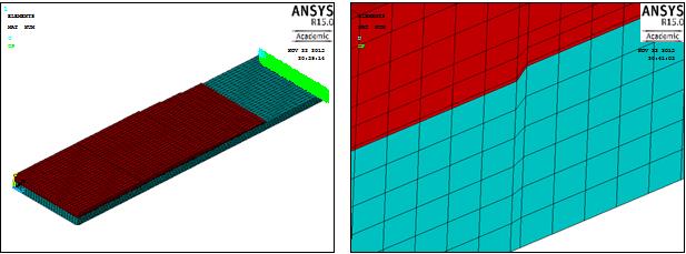
Figure 1.21: Curing of co-bonded patch.

Symmetrical And One Sided Configurations

In terms of configurations, the repair can be either applied to both sides of the defect or to one side. In fact the most favourable configuration is the installation of a patch symmetrically on both sides of the defect, as this alleviates the secondary bending effects that are manifested in the one sided repair due to the eccentricity of the neutral axis when it is axially loaded. The benefits of a double sided repair become more important in the extension of the fatigue life of cracked components, as it will be discussed later.

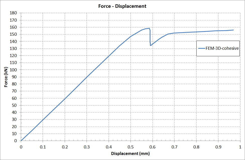
Nonetheless, in most applications it is simply not possible to install a symmetric configuration, as the area from the other side might be inaccessible, plus a double sided repair increases the time, cost and preparation actions required and might be difficult to be identically replicated from both sides.

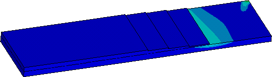
1.5 Loading / failure and analysis of composite patches The possible failure mechanisms in a bonded composite repair are shown schematically in Figure 1.22. Failure can occur either in the metal substrate, in the interface or/and the adhesive between the two different materials, or in the composite laminate. Therefore it is crucial to define prior to the design of the repair, which are the acceptance criteria for each one of the aforementioned types of failure, as, for example, partial debonding does not necessarily denote failure of the repair if the load can still be effectively transmitted from the substrate to the composite. Examples of failure criteria for the metal substrate are yielding, fracture, excessive deformation and failing to arrest the existing crack in the metal substrate. It is paramount that the engineer understands how the repair interacts with the remaining structure, as a wrong design might shift the existing problem or give way to new defects in other adjacent areas.

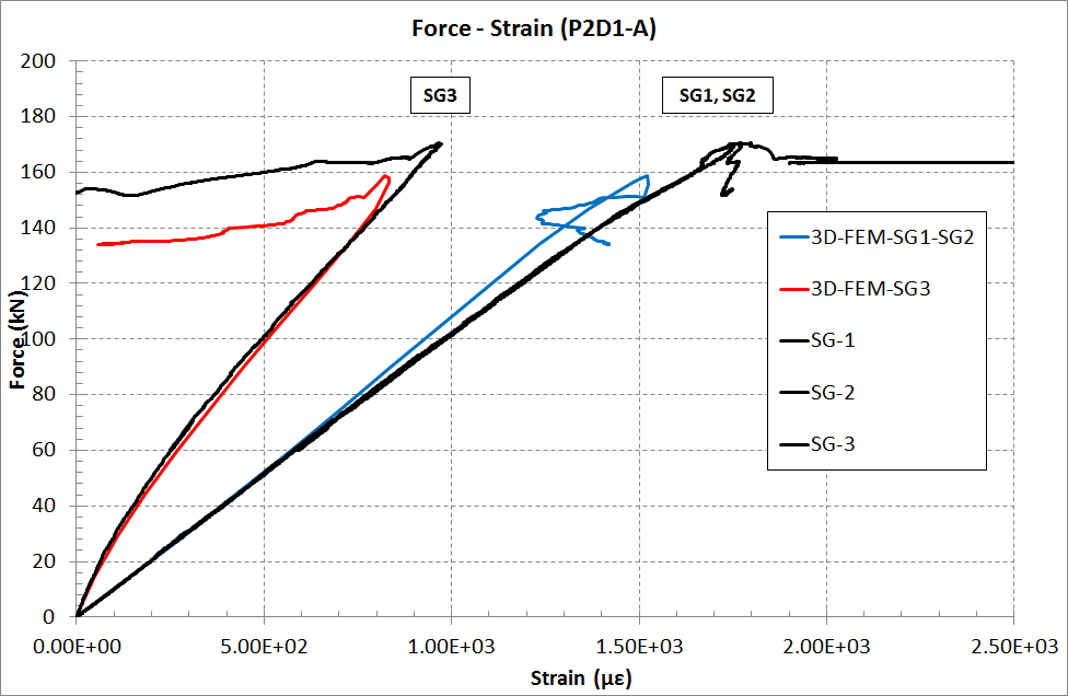
A well designed bond will rarely fail within the laminate, as this would mean that the strength of the composite is lower than the shear strength of adhesive or the interface. The most common failure types are crack extension in the substrate or/and extensive debonding.

As already stated, the main task of the composite patch is to bear part of the load acting on the steel structure. The load transfer between the substrates is achieved via the adhesive or the bimaterial interface. In other words the loads acting on the repair are governed by the acting load on the underlying steel substrate. As structural elements of marine structures are characterized by small thicknesses compared to their width and length, the loads acting on these are predominantly planar loads induced by axial and shear forces, bending moments and their combinations.

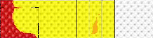
Figure 1.22: Types of failure in composite patch repairing (McGeorge et al, 2009). These forces and moments are the result of loads which are influencing the ship structure in primary, secondary and tertiary level (Hughes 2010). Quantification of the exact loading acting on a structural member is a complicated task, as some loads act in more than one level. Furthermore, the loading might be cyclic with frequency and amplitude governed by the location of the repair and the operating conditions. Due to the nature of such loads along with the fact that these will undoubtedly vary during the service life of the significant research both experimental and numerical focusing on the durability and failure of bonded composite to metal specimens. These have been mainly emanating from the aerospace industry investigating the effectiveness of composite patches on aluminium but also applications focusing on steel substrates and marine structures exist. In particular, Lam et al (2010) and Liu et al (2007) have performed research focusing on the proper identification of loading and failure modes with the use of finite element modelling, and the efficiency of patches in rehabilitating corroded plates and extending the fatigue life of cracked steel plates.

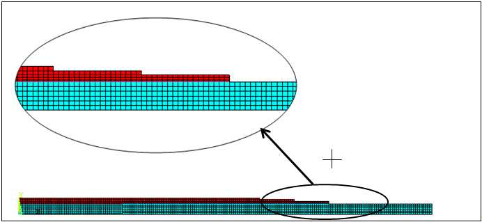
The design parameters that have been systematically examined are: the effect of the geometrical parameters of the patch i.e. the shape, thickness, length and width, the role of the stacking sequence and the effectiveness of each configuration in reducing the stress intensity factor (SIF) of the cracks in the metallic component (Xiong and Shenoi 2008, Hosseini – Toudeshky and Mohammadi 2007). In all cases it was proven that the patch was able to extend the fatigue life ranging from 2 up to 20 times compared to the unrepaired cracked plate, depending on the experimental configuration (Chung et al 2003, Seo and Lee 2002). The results were more prominent in the case of thicker patches and thin plates (Wang and Pidaparti 2002) and double sided repairs (Belhouari et al 2004, Megueni and Lousdad 2008, Liu et al 2009). This is attributed to the reduction of the stress intensity factor through the crack thickness (Megueni et al 2003-a, Bachir Bouiadjra et al 2002) which, in the case of one sided repairs, is not uniform leading to curved crack fronts. This phenomenon revealed the question of defining a representative value of the stress intensity factor for the assessment and design of repairs in cracked components. Researchers dealing with this issue have proposed different modelling and averaging techniques employing finite element modelling (Bachir Bouiadjra et al 2002, Umamaheswar et al 1999, Seo and Lee 2002, Megueni et al 2003-a). Lee and Lee (2004) used a successive crack front updating technique to capture the skewed crack front with the use of finite element modelling and successfully compared it to experimental results obtained for different metallic plate thicknesses (Figure 1.23). Toudeshky et al (2006, 2009) used the obtained mid plane SIF values for thin panels to predict the fatigue life of thin aluminium panels, however this proved to be problematic in the case of thicker plates. A different approach by measuring the SIF in a specific position of the skewed front was suggested by Hosseini – Toudeshky and Mohammadi (2007), based on the results from their experimental campaign.

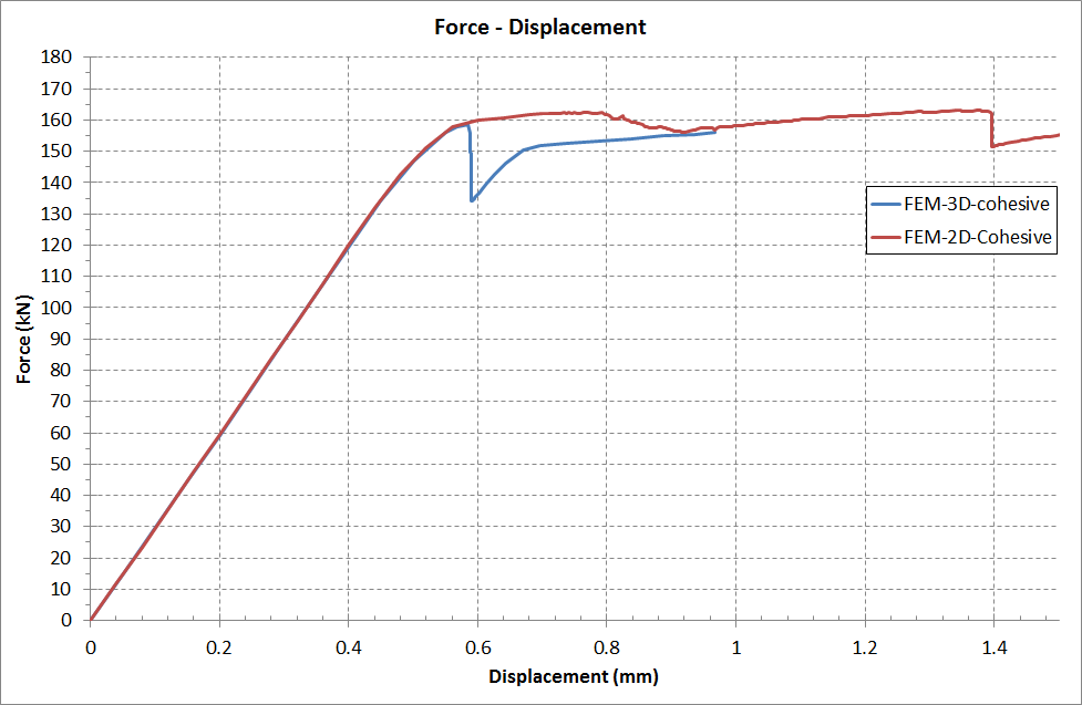
To better understand the interaction between the crack evolution in the base material and the repair configuration, the debonding effects have to be studied and understood. It has been observed that local debonding occurs in the vicinity of the crack tip, preceding it as the crack grows in the base material. Its extent relies on the given configuration, loading and the achieved quality of the bondline. The debonding around the crack area and the crack growth are interdependent, as the stress concentration and local plasticity in the crack tips in conjunction with the fact that the patch is more loaded above the crack region leads to the local debonding. This in turns redistributes and gives rise to the stresses acting in the vicinity of the track tip and simultaneously redistributes the load in the repair. This continues until either there is extended or total debonding of the two substrates or until the crack length exceeds the width of the repair.

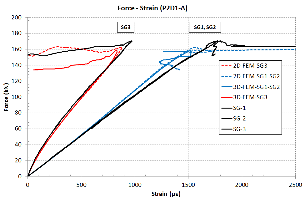
The importance of considering debonding has been highlighted by Mall and Conley (2009) and Papanikos et al (2005, 2007), who used progressive damage modelling techniques to simulate these effects (Figure 1.24). Figure 1.23: Skewed crack front in one sided repaired specimens (Lee and Lee, 2004).

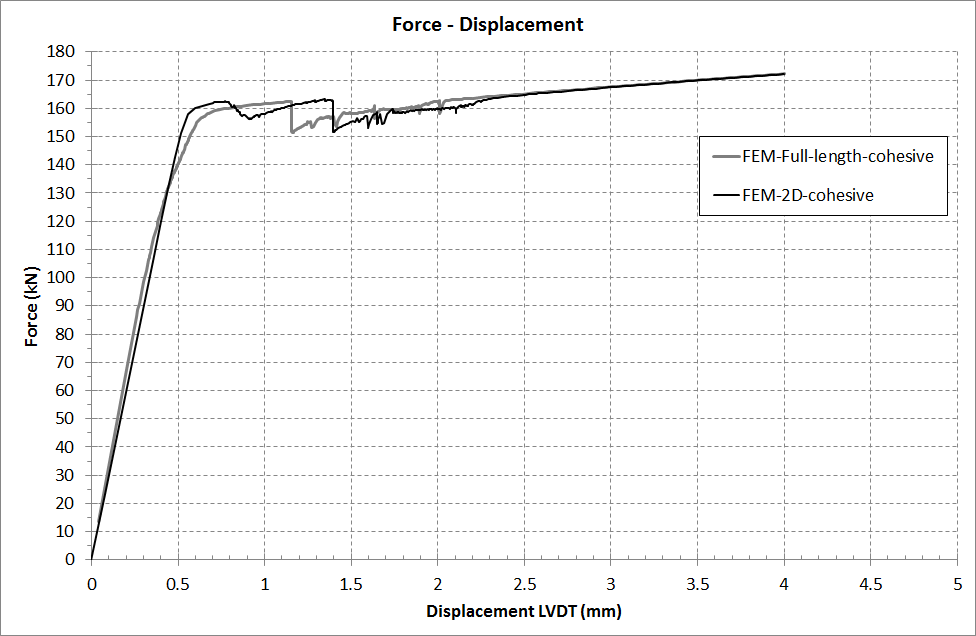
Figure 1.24: Numerical model depicting debonding evolution (Papanikos et al, 2005). 1.6 Non destructive evaluation, inspection and structural health monitoring As only limited in field experience on the long term performance of such repairs in marine applications exists, it is paramount that structural health monitoring and robust inspection techniques are applied to monitor the performance of the repair and possible evolution of damage in the substrate. Another challenge relies to the fact that being a hybrid construction, a practical solution is sought that would enable the monitoring of all involved materials i.e. metal, composite and the bond between these two. Different real time monitoring systems are available and could be employed to monitor the repair offering significant advantage in terms of reliability of the structure and minimizing periodic inspection requirements. There is a plethora of different non-destructive evaluation techniques which enable the monitoring of different types of flaws, however a significant part of these are difficult to implement on the field or not yet possible to form automated solutions.

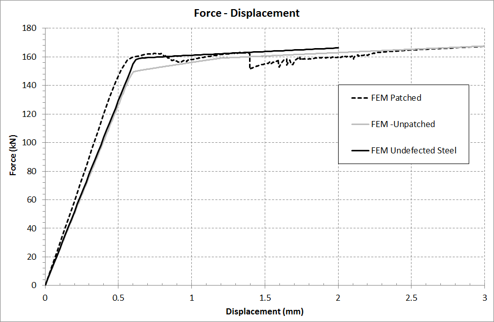
Strain Gages

Strains are mostly measured with electrical strain gauges. They constitute the simplest and most established solution for structural health monitoring with a broad range of existing commercial solutions to choose from and have been extensively used in laboratories and field applications (Grabovac 2009). Almost all strain gauges are glued to the surface of the material; it is theoretically possible to embed them inside a laminate, although there are several challenges associated with that approach, rendering it impractical. One very attractive solution is the combination of the strain-gages with the wireless technology, which counters the problem of extensive wiring that arise with the employment of traditional strain gages (Figure 1.25). Apart from strain gages, a variety of sensors can be combined measuring different features simultaneously (for example strains, temperature and acceleration), and special casings allow them to operate in aggressive environmental conditions and in different temperature ranges with substantial autonomy.

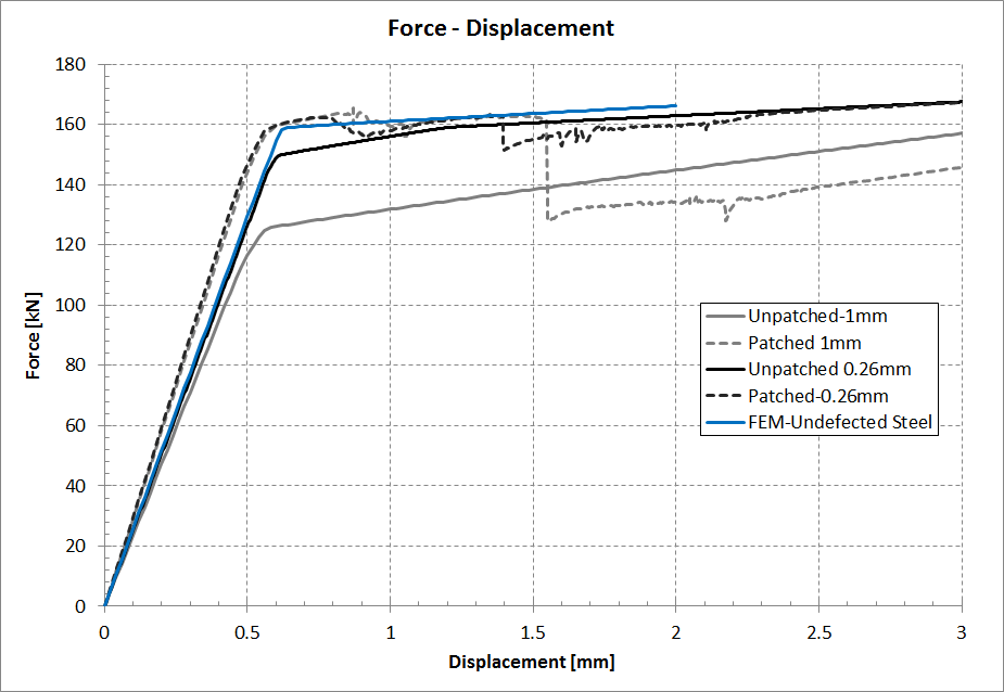
Figure 1.25: Commercial wireless sensor nodes.

Optical Fibres

Different optical fibre systems are available but unarguably Fibre Bragg Gratings (FBG) and Fabry-Perot have been more extensively used (Figure 1.26). Optical fibre sensors have a better long-term performance than strain gauges and are less sensitive to environmental attack. In addition, optical fibres can be embedded inside the composite laminate. This allows readings inside the laminate and the adhesive joint but also on the metal substrate. Examples depicting the potential of employing optical fibres for the monitoring of patch repairs are given by Baker et al (1999, 2009), McKenzie et al (2000), Jones and Galea (2002) and Takeda et al (2007). Careful consideration must be given to the position of the fibres in order to detect the changes in the strain field that might occur due to damage.

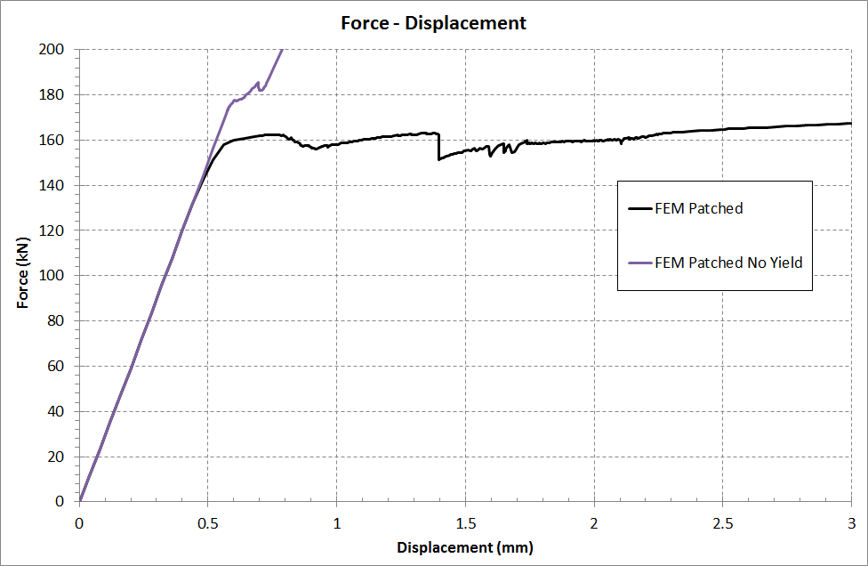
Figure 1.26: Optical Fibre system.

Ultrasounds / Acousto-Ultrasonics

Most of the ultrasound systems are used for periodic inspection and they are not permanently installed for industrial applications (Gieske et al 1998). The main principle of ultrasound is that a transducer sends an acoustic wave into the laminate and a receiver at a different position will detect this wave. Damage interrupts or modifies the flow of the acoustic wave and it is detected by a change in the characteristics of the wave or the time of flight. Moving transducer and receiver along the laminate allows scanning of the entire laminate.

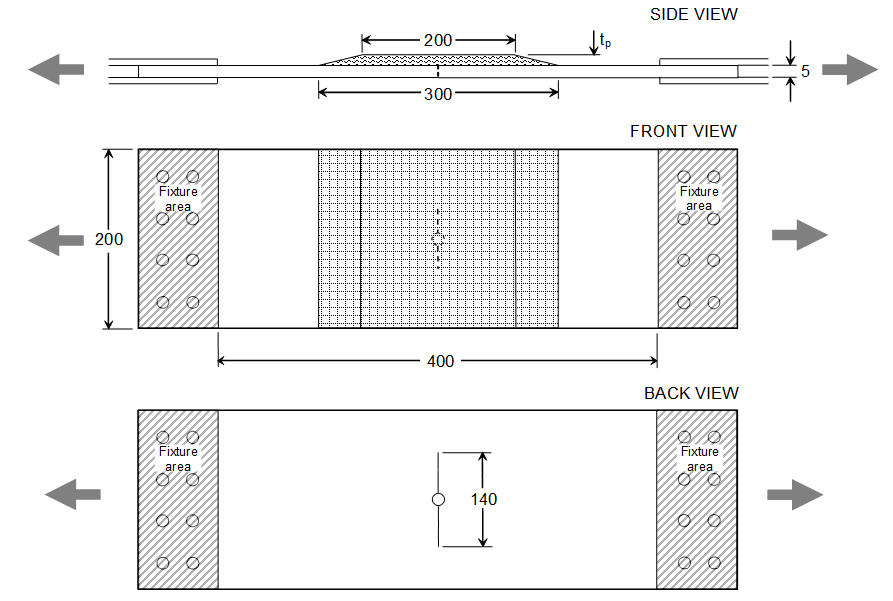
Moving can be done by hand or it can be automated. Independently of which method is used, the position of transducer and receiver needs to be known to find the position of the damage. Ultrasounds can detect defects/damage in the laminate, as well as cracks in metal substrate; however they are not reliable in detecting debonding in the adhesive.

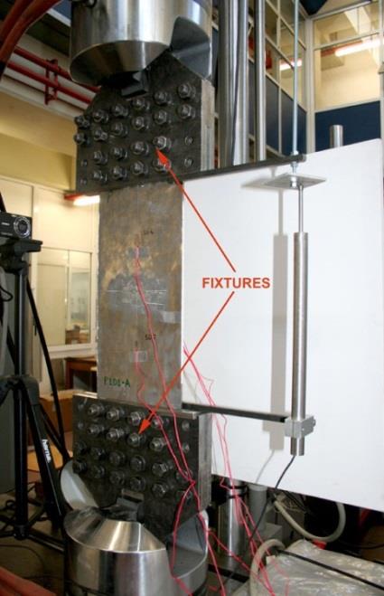
One of the methods used for the evaluation of the quality of the bond and the patch within the framework of this thesis was based on acousto-ultrasonics. The acousto-ultrasonic inspection is a fairly new technique that can be used to detect debonding. The difference to ultrasonic techniques is that the wave sent through the material has a much lower frequency than ultrasound. This low frequency gives in principle less resolution than the ultrasound method, but it has proven to be a reliable method to detect debonding both at the laminate and the steel/composite interface (Karatzas et al, 2014).

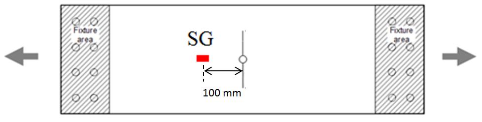
The Co-Patch Project

the Co-Patch research project funded from the European Community's Seventh Framework Programme (FP7/2007-2013) under grant agreement n° 233969 (www.co-patch.com). The scope of the project was to investigate the suitability and effectiveness of the composite repair method for the rehabilitation of large steel structures, focusing on marine and civil engineering structures.

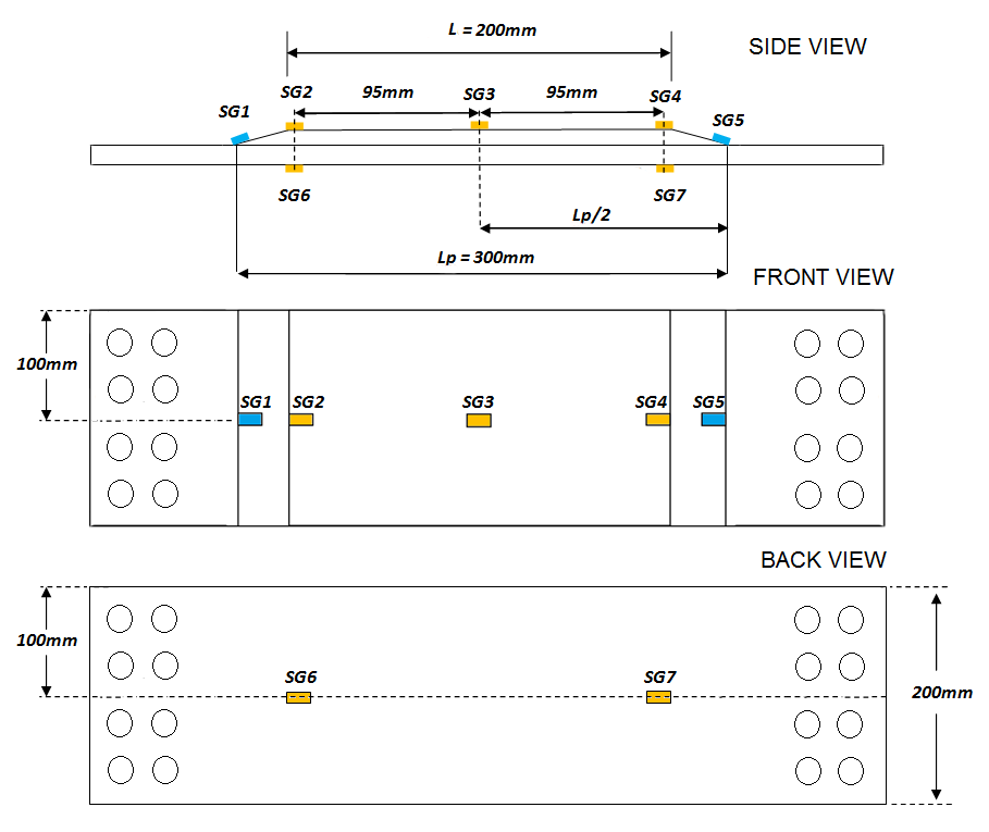
The project consortium consisted of fifteen different organizations from eight European countries. These are presented in Figure 1.27. Among these, the following were involved in the specimen preparation, manufacturing and testing for the experimental procedures that will be described in Chapters 3, 4 and 5 of this document.

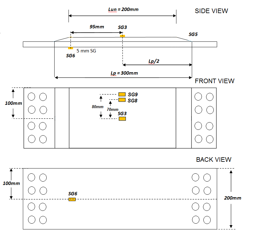
AS2CON is a research, development and application enterprise based in Croatia. They were responsible for the surface treatment and vacuum infusion of the composite patches for the manufacturing of the specimens subsequently tested under static and fatigue loading.

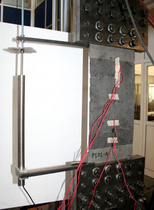
AIMEN is a research and development centre based in Spain. AIMEN undertook the task of testing the notched specimens in tension whose ultimate load exceeded the capacity of the testing machines available at NTUA’s facilities.

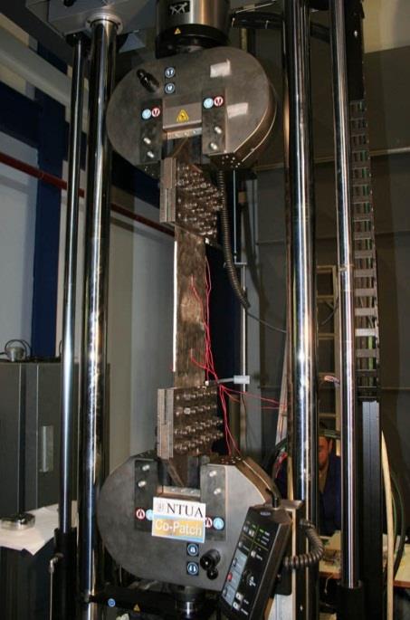
For the material characterization of the selected material configurations ENP, NTNU, UM and AS2CON were involved in the production of the specimen. ENP and UM are shipyards focused on the production of and Technology.

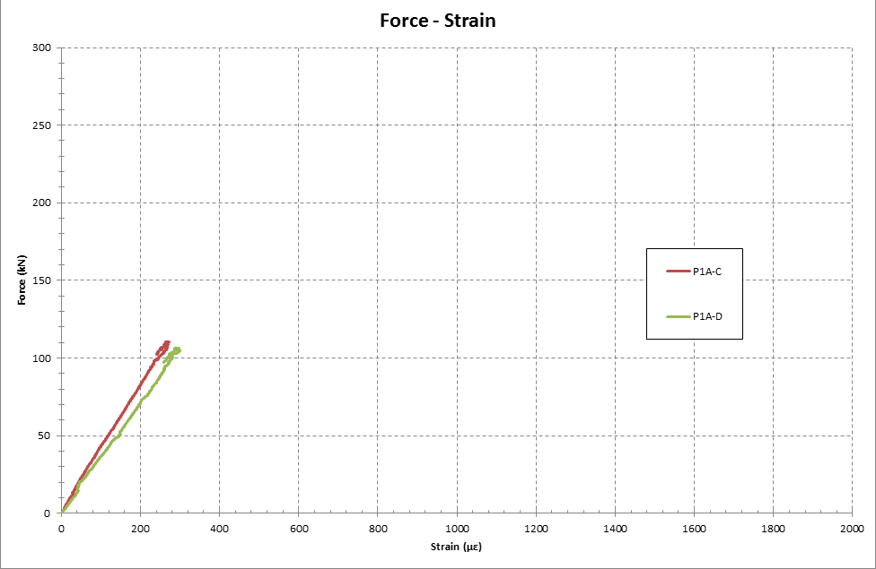
characterization of the steel that was used in the project. Figure 1.27: Co-Patch project partners. This dissertation emphasizes in presenting the most conclusive results and does not include all the research activities conducted for the project by the author as a member of the NTUA team in the project.

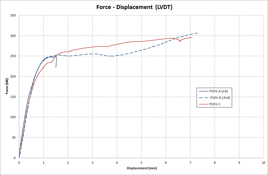
of typical defects found in marine steel structures namely cracks and corrosion. The main scope is, having demonstrated their potential, to further comprehend how specific parameters govern their efficiency on realistic operating conditions and to propose a straightforward design assessment methodology based on analytical tools, derived from Linear Elastic Fracture Mechanics for bimaterial interfaces. These simple analytical tools are to be utilized by design engineers and researchers for the evaluation, design and analysis of composite patch repairs and other similar adhesively bonded applications.

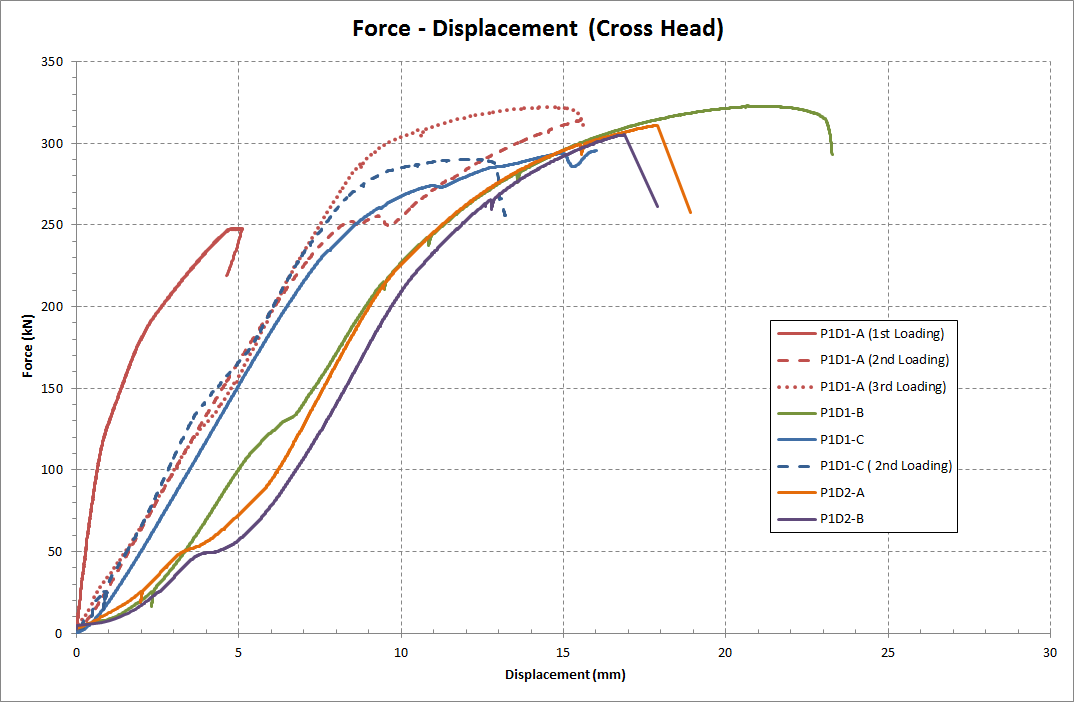
To achieve the aforementioned goals a combined experimental, numerical and analytical approach has been followed varying from medium scale, i.e. defected steel plates rehabilitated using composites under static and fatigue loading, to large scale study cases, such as the creation and analysis of a three compartment model of an AFRAMAX tanker using the Finite Element Method.

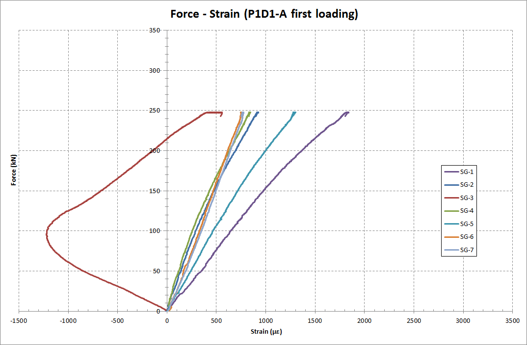
structures having addressed critical issues associated with their effectiveness, durability and inspection methods and a simple analytical design procedure is proposed.

Follows:

Experimental and Numerical Investigation of Repaired Corroded and Notched Plates under Static Loading In these chapters, an experimental campaign involving one selected composite material system have been undertaken showing the effectiveness of the repairs. A series of midscale static tests have been performed in defected steel plates, namely in corroded and notched plates. All plates have been repaired with the selected composite material system and were tested in tension. Additionally, different health monitoring and non-destructive evaluation methods have been applied to assess the quality of the repair both after installation and during operating conditions. Moreover, the effect of different aging scenarios has been investigated. Finally, 2D and 3D finite element models have been created using cohesive zone modelling, whose results are in very good agreement with the experimental findings. Results showed that the repair could reinstate the initial state of the structure and that failure was preceded by yielding of the steel substrates.

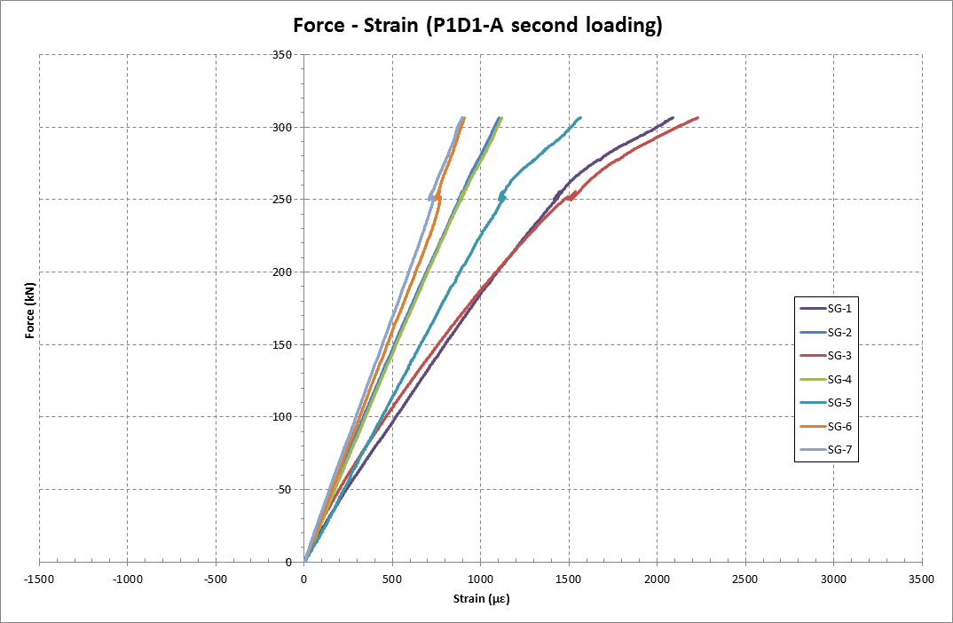
Experimental Investigation of Repaired Cracked Plates Subjected to Fatigue Loading Cracked plates on which composite patches have been installed were experimentally investigated under fatigue loading. Two different surface preparation methods have been investigated i.e. sand blasting and treating the surface with a needle gun. Once again, apart from the efficiency of the repair, health monitoring and non-destructive evaluation methods were employed. Additionally, the effect of different aging scenarios has been investigated. Results indicated that grit blasting led to better adhesion between the metallic and the composite substrates significantly extending the fatigue life of the specimens. The needle gun treatment on the other hand was able to extend the fatigue life in most cases but to a smaller extent.

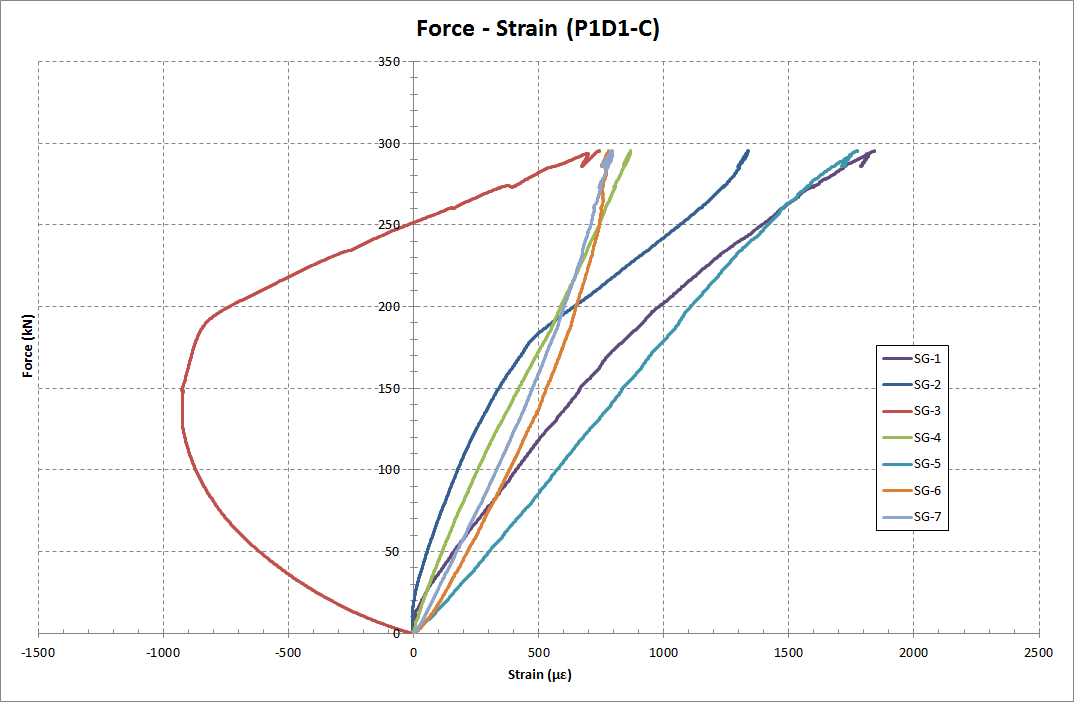
Numerical Simulations Employing a Three Compartment Model Additionally, a methodology for the assessment of cracked structural elements in marine structures has been proposed. This methodology is based on the implementation of the common structural rules for oil tankers with the use of user subroutines and finite element modelling. Numerical investigations on the ability of the patch repair to reduce the stress intensity factor of cracks in the structure have been performed.

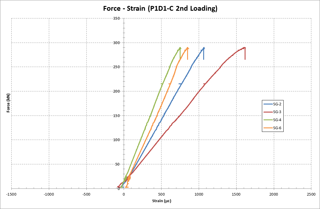
Parametric Investigation for the Design of Composite Patches and Design Methodology At the end of this work, emphasis is given in the use of linear fracture mechanics in bimaterial interfaces to address the integrity of the repair. By expanding the already existing work on the field an analytical parametric study has been performed to quantify how key parameters affect the adhesive bond between the patch and the steel substrate. Following the parametric study and based on the major findings and knowledge gained throughout this dissertation a simple, time effective design evaluation procedure for this kind of repairs is proposed.

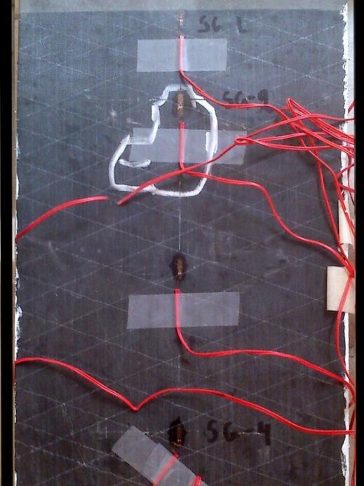
2. Introduction to Bimaterial Linear Elastic Fracture Mechanics

Ntroduction

The conventional design criteria are predominantly based on tensile strength, yield strength and buckling loads stemming from the widely known continuum mechanics approach. These criteria are adequate for many engineering structures but despite their usefulness, they are insufficient to interpret the creation and propagation of cracks in structures, hence a different approach should be sought. The field of mechanics concerned with the study of cracks in materials is called fracture mechanics.

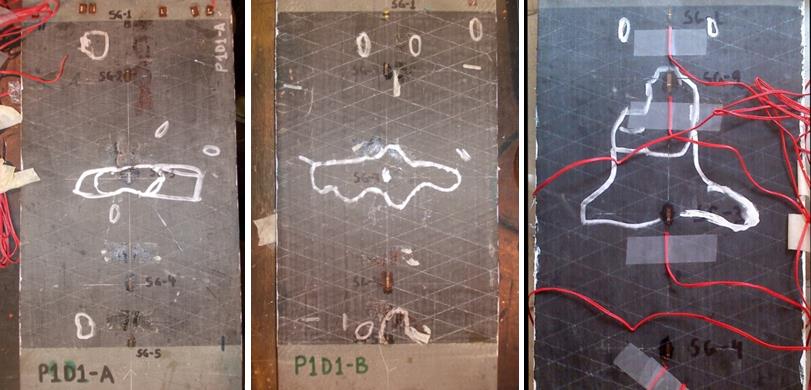
The problem of fracture has been concerning mankind since ancient times but it wasn’t until the 1920s by the work of Griffith (1921) that a systematic scientific approach was implemented to study the problem. Griffith applied the first law of thermodynamics to the formation of a crack. Namely, a crack can be formed (or an existing crack can grow) only if such a process causes the total energy to decrease or remain constant. Thus the critical conditions for fracture can be defined as the point where crack growth occurs under equilibrium conditions, with no net change in total energy. This approach was able to predict accurately the behaviour of brittle materials that obey Hooke’s law, such as glass, but failed to do the same for ductile materials where significant plastic deformation precedes failure. This was later made possible from the expansion of the original Liner Elastic Fracture Mechanics to the Elastic Plastic Fracture mechanics through the work of Irwin (1948) who managed to account for the energy dissipated in the material due to plasticity.

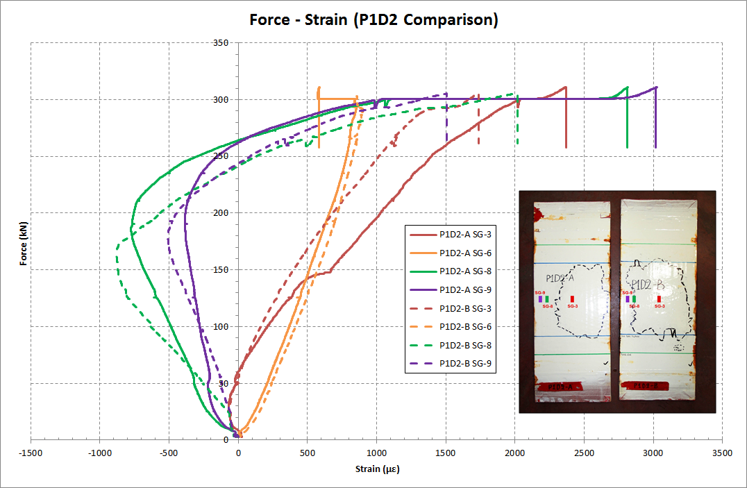
In this chapter basic concepts associated with the analysis and modelling of cracks in bimaterial interfaces that befall the Linear Elastic Fracture Mechanics theory are presented, as several of these have been employed throughout this dissertation.

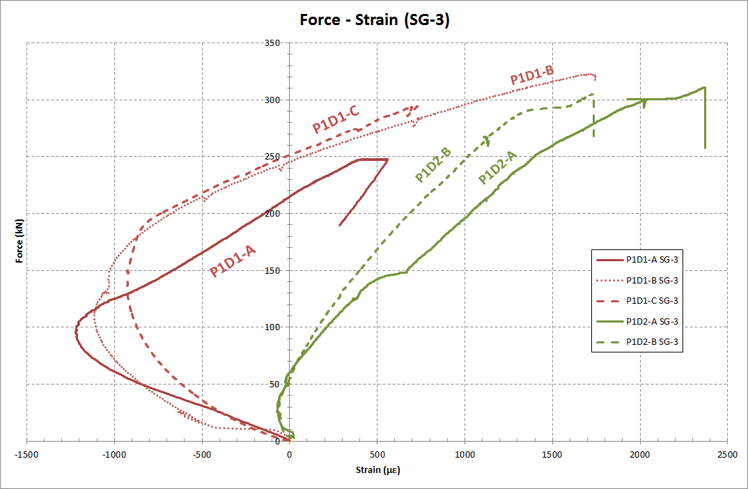
Inear Elastic Fracture Mechanics

According to Griffith’s theory, a flaw becomes unstable, and thus fracture occurs, when the strain energy change that results from an increment of crack growth is sufficient to overcome the surface energy of the material. Irwin extended this concept and proposed that the energy release rate, 𝐺, or the Griffith energy can be expressed as a measure of available energy for crack growth as expressed in Equation 2.1.

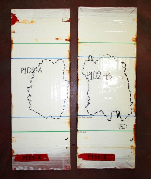
(2.1)

where 𝛱 denotes the potential energy and 𝑑𝐴 is the incremental area. When the potential energy becomes equal to the energy required for the creation of new surfaces (𝑊𝑠), Equation 2.1 expresses the critical energy release rate 𝐺𝑐 or Fracture Toughness (Equation 2.2). The energy release rate 𝐺 is the driving force for fracture, while 𝐺𝑐 is the material’s resistance to fracture

(2.2)

For certain cracked configurations subjected to external forces, it is possible to derive closed-form expressions for the stresses in the body, assuming isotropic linear elastic material behaviour. There are three types of loading that a crack can experience (Figure 2.1), namely: Mode I loading, where the principal load is applied normal to the crack plane, opening the crack. Mode II corresponds to in-plane shear loading and tends to slide one crack face with respect to the other. Mode III refers to out-of-plane shear and is not present in 2D analyses. A cracked body can be loaded in any one of these modes, or in a combination of two or three modes.

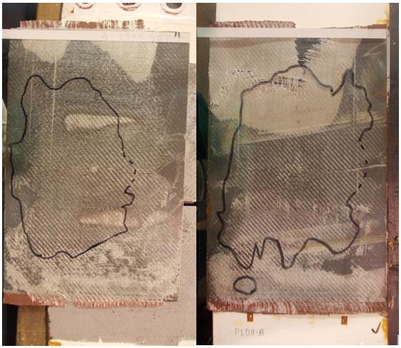
Figure 2.1: Loading modes. Irwin was also among the first to derive the singular stress field close to a sharp crack tip in 2D problems for a homogeneous isotropic elastic solid. For a polar coordinate axis with the origin at the crack tip, it can be proven that the stress field in any linear elastic cracked body is given by:

(2.3)

where 𝜎𝑖𝑗 is the stress tensor, 𝑘 is a constant and 𝑓𝑖𝑗 is a dimensional function of 𝜃 (see Figure 2.2). Figure 2.2: Stress field near a crack. The higher order terms depend on geometry and Am is the amplitude and 𝑔𝑖𝑗

(𝑚)(𝜃) Is A Dimensional Function

of 𝜃 for the mth term. In a mixed-mode problem (i.e., when more than one loading mode is present), the individual contributions to a given stress component are additive according to the principle of superposition. The stress intensity factor is equal to the constant k multiplied by √2𝜋 and is different for each loading mode. The relation between the stress amplitudes and the stress intensity factors for pure mode I (𝜎𝑥𝑦= 0) and pure mode II (𝜎𝑦𝑦= 0) respectively are listed in Equation 2.4:

(2.4)

The relationship connecting the stress intensity factors to the Griffith-energy is given in Equation 2.5

(2.5)

where 𝐸 is the efficient Young’s modulus for plane stress and plane strain conditions defined as 𝐸 = 𝐸 for

𝐸

1−𝜈2 for plane strain with 𝐸 being the Young’s modulus of elasticity of the material. The displacement field can be derived in a way similar to the stress field to describe the relative crack opening 𝛿2 and shearing 𝛿1 at a given distance behind the crack tip (Equation 2.6).

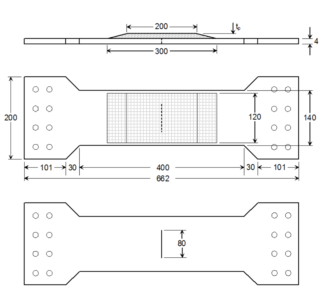
J Integral

The J-integral is a path-independent integral for the analysis of cracks developed by Rice (1968). The values of the J-integral denoted as 𝐽 are the energy release rate around a crack and are equal to the Griffith-energy when the Linear Elastic Fracture Mechanics approach is valid for the given problem (Equation 2.7).

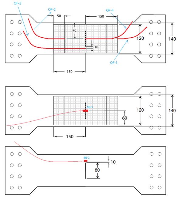
(2.7)

The J-integral, for an arbitrary counter clockwise path (𝛤) around the crack tip is given by Equation 2.8. A schematic of the J-integral is depicted in Figure 2.3

𝑢𝑖 = Displacement Vector Components

𝑑𝑠 = length increment along the considered contour 𝛤 The strain energy density is given by Equation 2.9

(2.10)

where 𝑛𝑗 is normal to the Γ contour around the crack tip. Figure 2.3: J-Integral schematic.

Bimaterial Fracture Mechanics

So far, basic concepts associated with Linear Elastic Fracture Mechanics have been described for homogeneous isotropic materials. In this section the expanded theory addressing inhomogeneous materials such as bimaterials is described. One important difference between homogeneous and inhomogeneous media should be outlined before proceeding. In the case of homogeneous materials, a crack will predominantly advance under mode I conditions and, even under mixed mode loadings, the crack will try to kink in a path where pure mode I loading exists. This is not the case in interfacial cracks advancing between two dissimilar materials. A crack in a bimaterial interface is restricted to propagating directly or along the interface. In this way it is forced to propagate in different mode mixities and not only under mode I.

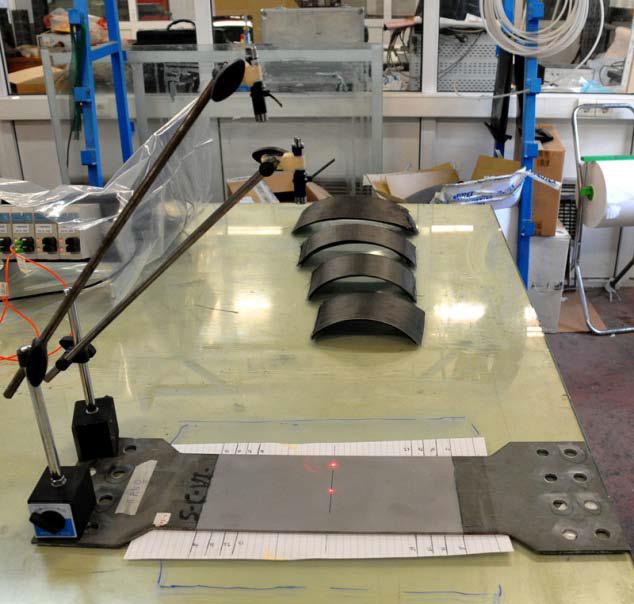
Consequently, the fracture toughness depends on the mode mixity and different values of fracture toughness are obtained with varying mode mixity. This is attributed to the contribution of mechanisms such as asperity contact which increases with increasing mode mixity. Additionally a high mode mixity tends to make the crack kink away in a microscopic scale which in turn increases the asperity and therefore increases the fracture toughness of the interface. This behaviour makes necessary the fracture toughness characterization Among the most important publications in bimaterial fracture mechanics are the ones from Hutchinson and Suo who were the first to establish a firm foundation for the analytical description of bimaterial fracture applied in different bimaterial problems and is not constrained to that particular application. Suo and Hutchinson (1988) analysed interface cracks between dissimilar isotropic linear elastic materials when subjected to bending moments and axial loads using the superposition principle. Suo (1990) presented a more general approach studying cracks between dissimilar anisotropic media. A recent study that is worth mentioning is that of Harvey and Wang (2012) who presented analytical theories for the mixed mode partitioning of one dimensional delaminations in composite materials, taking into account bending moments, axial forces and shear forces.

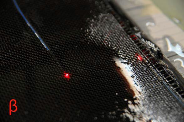
The Lekhnitskii-Eshelby-Stroh (LES) formulation (Lekhnitskii 1963, Eshelby et al 1953 and Stroh 1958) can be specialized to describe only the opening 𝛿𝑦 and shearing 𝛿𝑥 relative displacements of the crack flanks (Equation 2.11 and Figure 2.4) and in the same manner the 𝜎𝑦𝑦 normal and 𝜎𝑥𝑦 shear stress in front

Of The Crack Tip (Equation 2.12), As Follows:

Figure 2.4: Relative displacement at the crack flanks.

(2.12)

Where 𝐻11 and 𝐻22 are material dependent constants, and 𝜀 is the oscillatory index defined below. The mathematical expressions of these two parameters are given in Equations 2.15 and 2.16.

(2.16)

The subscripts 1 and 2 of the brackets refer to material 1 and material 2 respectively. 𝑆11 and 𝑆22 are components of the compliance matrix and 𝑛 and 𝜆 are non-dimensional orthotropic constants (Equations 2.13 and 2.14). The compliance components differ between plane stress and plane strain conditions, and for

(2.17)

These can be transformed to plane strain by Equation 2.18:

(2.18)

The oscillatory index 𝜀 mentioned in Equations 2.11 and 2.12 is given by Equation 2.19:

(2.19)

The term 𝛽 used for the calculation of the oscillatory index is the second Dundurs parameter for bimaterials. Dundurs (1970) observed that the elastic moduli dependence of a bimaterial system may be expressed in terms of two parameters 𝛼 and 𝛽. At this point it must be noted that the expressions of the Dundurs parameter are different for an isotropic bimaterial than for an orthotropic one. In the latter these are referred to as the generalized Dundurs parameters and are expressed by Equation 2.20 and Equation 2.21. When both substrates are isotropic the generalized expression of these parameters reduce to their isotropic form

(2.21)

The first Dundurs parameter measures the mismatch in the plane tensile modulus across the interface. The physical interpretation of the second Dundurs parameter is more complicated compared to the first one, representing a measure of the mismatch in the in-plane bulk modulus. Both parameters vanish when there is no mismatch, and both change signs when the same materials are used but are assigned to the opposite designation. The complex stress intensity factor K in Equation 2.12 is defined as:

(2.22)

It should be noted at this point that Equations 2.11 and 2.12 are similar to 2.4 and 2.6 defined for homogeneous materials, however the stress intensity factors 𝐾1 and 𝐾2, unlike the isotropic case, do not represent individual stress amplitudes for mode I and II. This is due to the contribution of the term |𝑥|𝑖𝜀 which leads to the mix-up of the traditional stress intensity factors (Equation 2.23). As a result of this mix-up, an opening of the crack flanks does not necessarily mean that 𝐾2 = 0, but rather that mixed mode condition is present with both 𝐾1 and 𝐾2 having values different from zero.

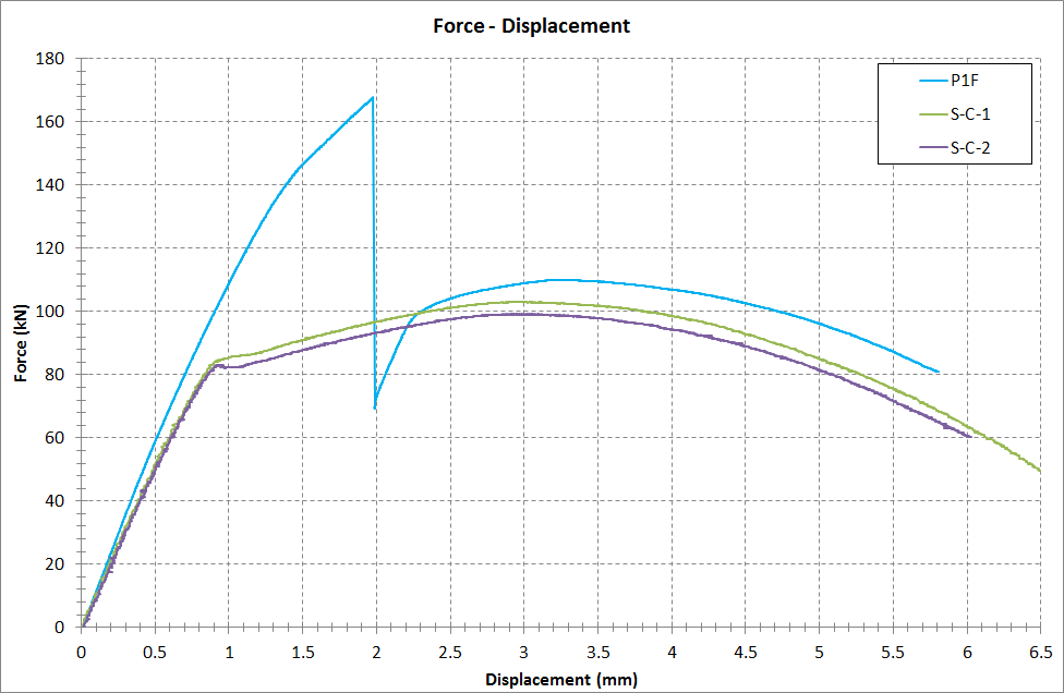
𝐾|𝑥|𝑖𝜀 = [𝐾1𝑐𝑜𝑠(𝜀𝑙𝑛𝑥) −𝐾2𝑐𝑜𝑠(𝜀𝑙𝑛𝑥)] + 𝑖[𝐾1𝑐𝑜𝑠(𝜀𝑙𝑛𝑥) + 𝐾2𝑐𝑜𝑠(𝜀𝑙𝑛𝑥)]

(2.23)

The complex intensity factor (Equation 2.21) can be related to the strain energy release rate as (Suo 1990)

(2.24)

Similarly, the strain energy release rate can be expressed in terms of the opening and relative sliding displacements of the crack flanks (Hutchinson et al 1992) as illustrated in Equation 2.25:

(2.25)

A way to quantify the mode mixity is by calculating the phase angle; however, there are different definitions of the phase angle depending on the bimaterial system and on the assumptions made by the analyst. The most commonly employed are concentrated in this section. In the case of homogeneous materials the mode mixity is defined based on the stress intensity factors (Equation 2.26)

(2.26)

which, for that particular case, is equivalent to Equation 2.27

(2.27)

However in bimaterial fracture mechanics the stress intensity factors do not correspond to pure modes I and II. Therefore Hutchinson and Suo (1990) defined the mode mixity using the expression of Equation 2.28:

(2.28)

where ℎ is the characteristic length of the problem. This parameter has no physical meaning and its value is chosen so as the mode mixity 𝜓= 0 corresponds to the minimum value of the Griffith energy, and different values of this parameter lead to a phase shift. Alternatively to Equation 2.28, the mode mixity can be expressed as a function of the crack flank displacements 𝛿𝑦

(2.29)

The phase angle formula can be simplified by setting the oscillatory index 𝜀= 0. In this way, the following reduced form can be assumed (Equation 2.30), which is more practical:

(2.30)

The reduced formulation can be rewritten using the Griffith energy mode I and II as shown in Equation 2.31

(2.31)

It is obvious that for the same energy release rate, different values of mode mixity can be obtained depending on the selected definition. The difference between the full formulation and the reduced one is in effect a phase shift caused by the presence of the two additional terms that are dependent on the oscillatory index in the full formulation expression. This phase shift makes the interpretation of the phase angle somewhat non intuitive as the physical meaning granted by the first term of Equation 2.29 is obscured by the phase shift. Therefore the reduced formulation is more appealing as it captures better the physics of the problem denoting the ratio of mode II energy release rate to mode I. Interpreting Equation 2.31, it follows that a phase angle of 0o denotes a pure mode I condition and a phase angle of 90o a pure mode II. In the case when the energy release rates for both modes are equal, the phase angle is equal to 45o. Bearing these observation is mind, cases where the phase angle is between 0o and 45o are referred to as mode I dominant as the energy release rate due to mode I loading is greater to the energy release rate caused by mode II loading. Inversely, cases with phase angle values between 45o and 90o are referred to as mode II dominant, meaning that the mode II loading contribution in the total energy release rate is greater than the one due to mode I loading. From the defined mode mixities, the full and reduced formulations have been used throughout this thesis.

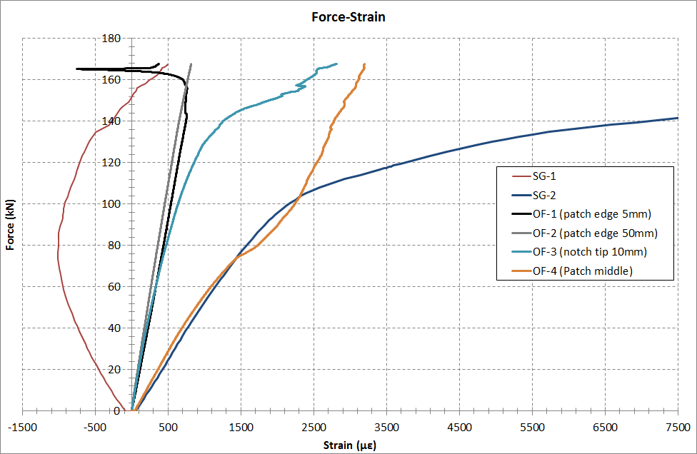
Ntroduction

An advanced modelling technique to simulate the evolution of damage between adhesively bonded interfaces is cohesive zone modelling which befalls the field of damage mechanics. Damage mechanics permits the simulation of the initiation, progressive damage and fracture at a predefined crack path constituting it ideal for the analysis and simulation of damage in bimaterial interfaces where the crack path is already known. This field is still under intense development regarding more accurate and robust modelling techniques, different models to cover the range of different available adhesive systems and their behaviour, and also to eliminate existing convergence issues. Another advantage of this modelling approach is that it is heavily implemented in commercial finite element software and has become the most widespread method of predicting damage. Additionally cohesive zone modelling can be implemented to model both brittle and ductile behaviour making it an invaluable tool for the latter where Linear Elastic Fracture Mechanics is no longer valid and the elastic plastic fracture mechanics is cumbersome to implement analytically.

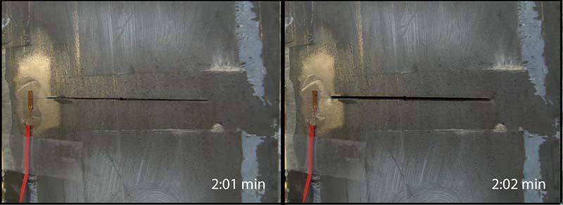
The cohesive zone modelling technique consists of establishing traction-separation laws to model the interface behaviour. These laws are established between paired nodes of cohesive elements and can be used to connect superimposed nodes of elements representing the different substrates, simulating a zero thickness interface which is referred to as the local approach, or they can be applied in non-contacting mediums simulating the entire adhesive bond which is referred to as the continuum approach (Yang et al., 2001, Kafkalidis and Thouless, 2002).

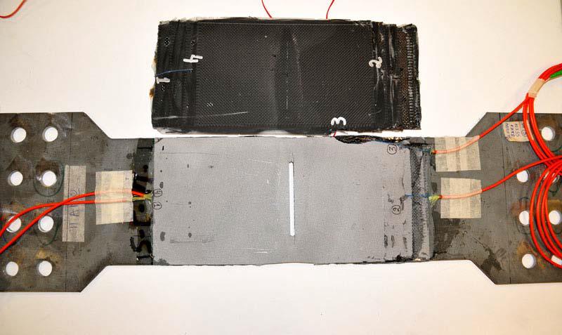
The use of cohesive zone models (CZM's) coupled to conventional FE analyses is the most widespread method of predicting static or fatigue damage uptake in structures (Tvergaard and Hutchinson, 1992; Tvergaard and Hutchinson, 1993; Yang et al., 1999; Yang et al., 2000; Yang and Thouless, 2001; Campilho et al., 2005; Campilho et al., 2007).

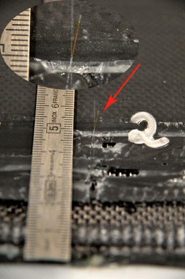
Ohesive Laws

The cohesive law, or traction-separation law, relates the tractions 𝜎 acting on the two planes of the cohesive elements with the corresponding separations 𝛿 for each loading mode; meaning, that the local normal stress 𝜎𝐼 and local shear stresses 𝜎𝐼𝐼 are associated with the normal crack opening 𝛿𝛪 and with the

(2.32)

The traction separation law for each mode is defined employing specific experimental procedures. Through these experiments the critical energy release rate can be calculated under pure or mixed mode loadings. By differentiating the critical energy release rate by the normal opening for mode I and by tangential opening for mode II at the precrack tip, the respective pure mode laws are defined. Inversely, this means that the area enclosed by the traction separation law should be equal to the critical energy release rate measured.

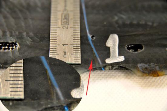
In the case of pure mode loading there is no interaction between the cohesive laws, meaning that the normal cohesive stresses depend solely on the normal opening displacement for the case of pure mode I and the shear cohesive stresses depend on the tangential crack opening in the case of mode II loading. The cohesive laws for pure mode I and pure mode II is also what constitutes the required input in most finite element software. For the mixed mode, the two pure modes are coupled through a failure criterion that gives the critical combination of opening and shear displacements at which the tractions in both modes fail simultaneously. The variation of the fracture energy from mode I fracture to mode II fracture has been demonstrated through mixed-mode fracture specimen (Banks-Sills and Bortman, 1986) and delamination testing (Reeder and Crews, 1990; Benzeggagh and Kenane, 1996). The most commonly employed mode mixity law is the power law (Wu and Reuter 1965) illustrated in Equation (2.33) with superscript values

(2.33)

general, a cohesive law is described by two parts, a traction strengthening part and a traction softening one following the latter. The most commonly used are of the following shapes: bilinear, exponential and trapezoidal. However it must be pointed out that the shape of the traction separation law does not significantly affect the results of the analysis (Alfano 2006). The bilinear law is depicted in Figure 2.5 and its analytical expression is presented in Equation 2.34:

(2.35)

𝐺𝑐 represents the fracture energy dissipated during the complete debonding process and is equal to the area enclosed by the 𝜎−𝛿 curve and 𝐾0 is the initial penalty stiffness. Figure 2.5: The bilinear traction separation law.

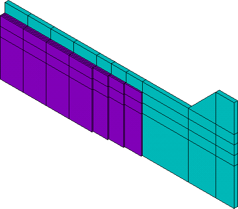
Regarding the traction strengthening part, two different approaches exist i.e. the intrinsic and the extrinsic approach, (Kubair and Geubelle, 2003). In the intrinsic approach the slope of the initial strengthening part, increases denoting an increasing resistance as the cohesive surfaces move relative to each other. At a given separation 𝛿𝑜 the maximum cohesive traction 𝜎𝑐 is reached. After that point the traction softening starts and tractions reduce following a linear, exponential, or polynomial fashion depending on the shape of the softening law, until the critical separation value 𝛿𝑐, where the tractions have reached zero which leads to the tractionless separation of the cohesive surfaces simulating in that way a physical crack. Needleman (1987) was the first to introduce the intrinsic approach within the context of finite element methods by using a polynomial form for the traction–separation law in the modelling of void nucleation associated with particle debonding.

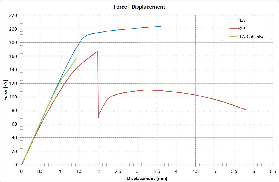
The extrinsic approach assumes that there is no strengthening part and that the cohesive law consists solely of the traction softening part. Nevertheless, due to numerical purposes a very steep initial strengthening part is included and as it represents a minor fraction of the area under the traction separation law, the represented critical energy release rate is not affected. The most commonly used extrinsic laws are the triangular, linear-parabolic and exponential (Alfano and Crisfield, 2001), linear-parabolic (Allix and Corigliano, 1996), polynomial (Chen, 2002) and exponential (Chandra et. al, 2002). The CZM has been extensively used for the simulation of adhesively bonded structures. (Chai, 1988; 1995; Ikeda et al., 2000; Yan et al., 2001; Lee et al., 2004; Pardoen et al., 2005).

Depending on the adhesive bond under study, the analyst has to consider which approach is the most suitable one to represent the physical problem. In the case of co-cured bonding, the extrinsic local approach is favored, as there is no distinct adhesive layer joining the different substrates.

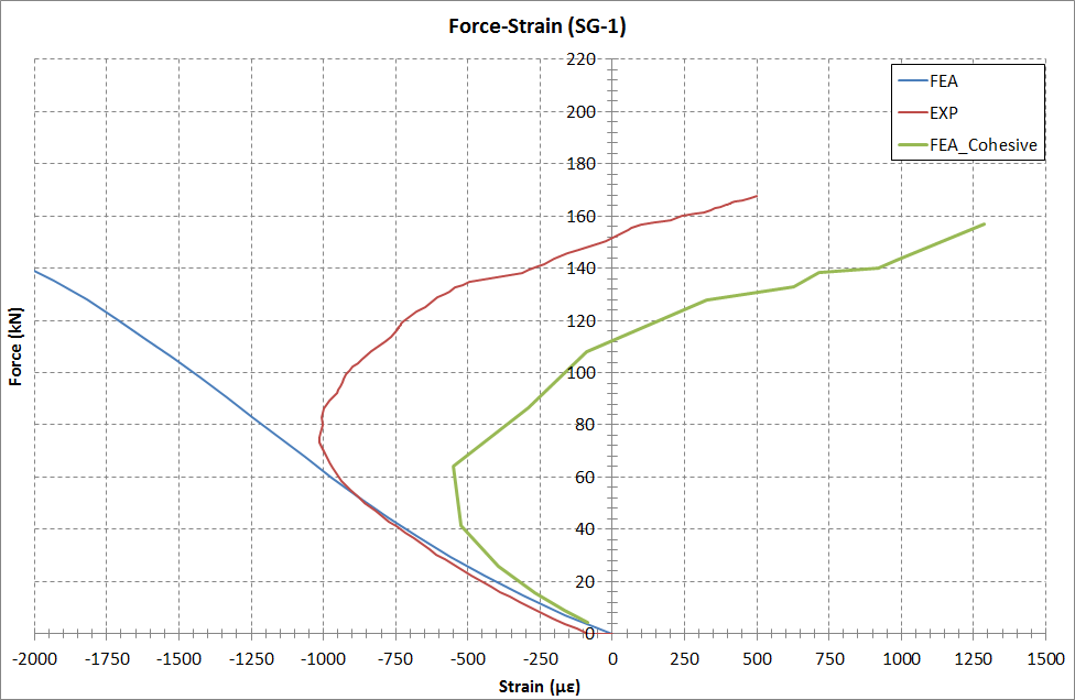
2.6 Experimental procedures for the measuring of the critical energy release rate in bimaterials For the implementation of Linear Elastic Fracture Mechanics and cohesive zone modelling experimental testing is required in order to measure the fracture toughness of the bimaterial system. As mentioned earlier, a crack in a bimaterial interface is restricted to propagating directly or along the interface. In this way it is forced to propagate in different mode mixities and not only under mode I.

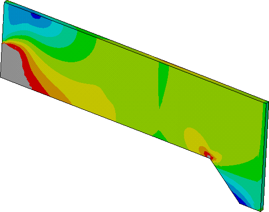
Having identified this behaviour, special attention has been paid to develop sound experimental and data reduction techniques for the correct measurement of the fracture toughness of bimaterials under different mode mixities using precracked specimens. These have been developed predominantly for the study of delamination in laminates and sandwich structures, where delaminations and debonding between the face skin and the core are prevalent. A few corresponding data reduction techniques are currently available (e.g.

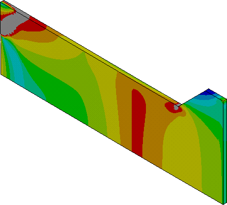
the property determination technique, the direct method and the inverse method) that enclose varying degrees of complexity and expected accuracy of the results. Some of the more widely used debonds test specimens include the Double Cantilever Beam (DCB) for measuring mode I, the End Notch Flexure (ENF) for measuring mode II and the Mixed Mode Bending (MMB) tests for measuring different mode mixities. The Mixed Mode Bending tests (Figure 2.6) can be considered as a superposition of the DCB and ENF tests and with a suitable loading lever length, different mode mixity ratios can be achieved.

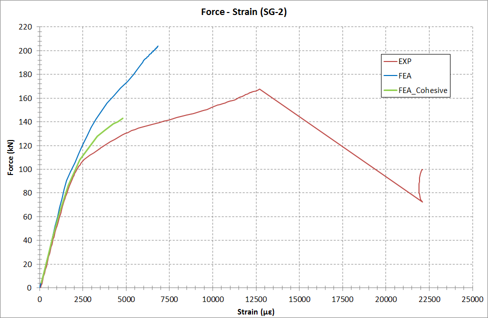
Figure 2.6: MMB geometry parameters and test setup (Carlsson 2014). However, few data and methods seem to exist for characterizing bonds between dissimilar materials. Lee et al (2010) performed Single Leg Bending tests on co-cured specimens under mode I and mode II dominant modes (Figure 2.7) and subsequently extracted the pure mode I and mode II fracture toughness with the use of numerical simulations. The materials used were unidirectional carbon fibres on steel which had been treated with emery cloth before bonding. The values obtained were 140 J/m2 for pure mode I and 280 J/m2 for pure mode II. Andersen and Echtermeyer (2005) performed DCB and ENF tests to characterize the adhesive bonding between grit blasted steel and a carbon epoxy system with a chop strand mat glass layer in the interface (Figure 2.8). The fracture toughness of the composite system for mode II is in good agreement with the values obtained by Lee as it was measured equal to 283 J/m2 with a standard deviation of 96 J/m2. The fracture toughness for mode I was measured equal to 593 J/m2 with a standard deviation of 108 J/m2. At this point it must be noted that examination of the surface after testing for these specimens indicated that there was quite a certain degree of matrix microcracking and delamination between the glass layer and the carbon laminate and that the debonding was not purely an adhesive one as resin remnants were found on the steel surface. And as such the measured fracture toughness is the resulting contribution Figure 2.7: Single leg bending tests performed by Lee et al (2010).

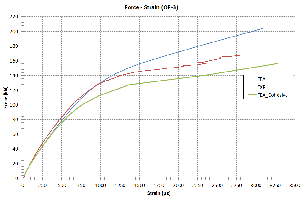
Figure 2.8: Partial adhesive failure of DCB specimens (Andersen 2005). A very promising experimental test is the Double Cantilever Beam with Uneven Bending Moments (DCB- UBM) (Sørensen et al 2006; Berggreen 2013). The principle behind this method is to create two different bending moments in the free beams of a DCB-UBM specimen. Two different setups exist, with the main difference being the way the moments are applied to the free beams of the specimen. The first one was developed by Risø national laboratories and employs two different moment arms, one at each side of the specimen. By applying the same loading in these arms, different moment ratios can be achieved (Figure 2.9, left). In the second type, the moment is generated by directly applying rotation with the use of rotational actuators (Figure 2.9, right). In both cases the specimen is restricted from rotation at the uncracked end but can freely move in the longitudinal direction.

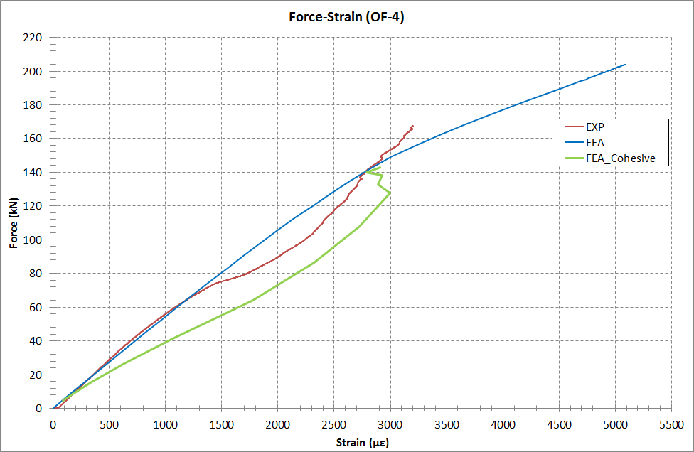
The main advantage of the DCB-UBM tests is that the energy release rate can be calculated without the need to measure the crack length during testing, which can be hard to achieve in an accurate way. Moreover, since there are no transverse forces transmitted to the specimen, the friction between the opening faces is reduced. Additionally, the desired mode mixity can be achieved directly from controlling the lever arms or the actuators and therefore, the same specimen can be used for all range of mode mixities.

Figure 2.9: DCB-UBM test rigs. 3. Experimental and numerical investigation of patch repaired

Ntroduction

The experimental program described in this chapter consists of static testing of plates which have been artificially corroded and subsequently reinforced with a one-sided composite patch. These specimens are referred to as P2 to differentiate them from specimens with different type of defect which are presented subsequently in Chapters 4 and 5 of this dissertation. The main objective is to experimentally prove in a systematic way that the use of a composite patch increases the static strength of a corroded steel structure.

Another objective is to provide solid and systematic experimental data, which are used to assess the effectiveness of the repairs. In parallel, the experimental results presented in this report are used to validate the developed finite element models. The tests are categorized in different groups according to the aging scenario. Defected unrepaired plates were also tested to evaluate the effectiveness of the patch.

Specimen Description

The geometry and main dimensions of the type plates tested are presented in Figure 3.1. The nominal thickness of the steel plates, ts, is 5 mm. The central orthogonal reference part of the steel specimen has length Ls equal to 400 mm and width Ws equal to 100 mm. A central area on one side of the plate having length 100 mm and width 80 mm has been subjected to artificial corrosion, by partially protecting the plate (using a special nylon sheet and special sealing tape, that can withstand the accelerated corrosion conditions), leaving the 100 x 80 mm area exposed, and subsequently placing the plates in an environmental chamber. The artificial corrosion procedure lasted for 250 cycles (≈83 days, see Table 3.1 for the details of each cycle). This time of exposure was deemed adequate for the study of the effects of corrosion and efficient for the time limitations of the project. Corrosion cycles were in accordance with ISO 14993:2001.

After this procedure the rust was removed and the corroded areas were treated using grit blasting. On top of the corroded area (front side), and after the surface preparation, a central composite patch of thickness tp, effective length Lp = 200 mm and width Wp = 100 mm, equal to the specimen’s width, was laminated. The total patch length (Lpt) is greater, equal to 300 mm, as it additionally includes the tapered edges of the patch.

Figure 3.1: P2 plates geometry. Table 3.1: Conditions of one accelerated corrosion cycle.

> 95% Rh

A total of ten (10) specimens were tested in this experimental campaign. Two of them, namely P2A-C and P2A-D were damaged unrepaired specimens. These served as a reference for the investigation of the effectiveness of the repaired cases. The remaining eight specimens were nominally identical from a geometrical and material perspective and were grouped in four pairs denoted as P2D1, P2D2, P2D3 and

P2D4.

After the lamination and curing of the patch, specimen groups P2D2, P2D3 and P2D4 were subjected to accelerated aging conditions into an environmental chamber according to ISO 14993:2001. The scope was to investigate the effect of the environmental conditions on the integrity of the repair. Sealing tapes were used to protect the edges that were later inserted in the fixtures (Figure 3.2). The specimens subjected to the aging process were exposed for 300 cycles (i.e. 100 days) under cyclic corrosion (including salt mist, dry and wet conditions in different temperatures) and were subsequently tested in tension. This time of exposure was considered satisfactory for the study of the effects of aging, without being overly time demanding.

Area

Figure 3.2: Six P2D (2 painted and 4 unpainted) specimens after 75 days in the environmental chamber. Cyclic aging testing is intended to be an accelerated way to perform salt spray tests than traditional, steady state exposures. Because actual atmospheric exposures usually include both wet and dry conditions, indicates that, with cyclic aging tests, the relative corrosion rates, structure and morphology are more similar to those seen outdoors. Consequently, cyclic tests usually give better correlation to outdoors than conventional salt spray tests. They are effective for evaluating a variety of corrosion mechanisms but there is no direct way to correlate the endured aging cycles with in service conditions.

From the aforementioned groups, specimens P2D3-A and P2D3-B have been painted with typical marine grade paint before being placed into the salt spray chamber. The rationale behind this was to investigate whether the application of a typical marine coating would sufficiently protect the repair from the detrimental environmental conditions. The specimen nomenclature is presented in Table 3.2. Naturally there were some minor variations in the geometry of the specimens from the nominal values presented above. For this reason, the exact geometry of the specimens is presented in Table 3.3 below.

The specimens’ width exceeded that of the grips of the testing machine. Therefore, in order to achieve the uniform loading of the specimens along their width, special steel fixtures were designed and manufactured. The specimens were positioned in the fixtures and kept in place with the aid of 16 M16 bolts, through holes specifically opened for this purpose. These friction grip fixtures were designed to accommodate specimens with various thicknesses (from 2 to 20 mm) and widths (from 100 to 300 mm). In order to achieve complete contact between the fixtures and the specimens, steel sheets with various thicknesses (from 1.5 to 5 mm) were used as fillers. The fixture-specimen assembly was subsequently mounted to the testing machine (Figure 3.3).

Table 3.2: Nomenclature of P2 specimens.

Days

Table 3.3: Dimensions of P2 specimens.

-

1Not measured. Figure 3.3: Fixture specimen assembly mounted for testing.

Aterials And Manufacturing Procedure

The experimentally derived tensile properties of this specific steel were 203 GPa for the Young’s modulus and 314.6 MPa for the yield stress. The material characterization tests were performed by UniS (Zhang and Chryssanthopoulos, 2011). The composite material system used for the manufacturing of the patches is Carbon/Epoxy using the vacuum infusion method. The mechanical properties of the laminate are listed in Appendix A. The specimens were fabricated in two steps by the Co-Patch project partner AS2CON using CST 200 carbon unidirectional fibres with area density equal to 200 g/m2 provided by SGL GROUP. The number of layers for each specimen was 16 (made in two stages, 8+8 plies). The resin used was LH 288 Epoxy resin by HAVEL and it was made by mixing Aerosil (hydrophilic Fumed Silica) and micro balloons. A 280 g/m2 E-glass woven roving, twill weave by AEROGLASS was used to prevent galvanic corrosion between the carbon fibres and the steel substrate. The epoxy resin hardener was H283 by HAVEL. The mixing ratio of resin and hardener was 100:19. The specimens were produced using the vacuum infusion method. The resin inlet was placed in the middle, and vacuum outlet was placed around the plate as seen in Figure 3.4. . The specimens were produced under the vacuum of -0.75 bar. Prior to infusion, all materials were heated to the production facility room temperature to enhance the curing of the resin, and resin flow.

The environmental conditions at the production facility were 35ºC and 29% humidity for the first step and 35ºC and 34% humidity for the second. Figure 3.4: Vacuum infusion setup (figure provided by AS2CON).

Prior to the vacuum infusion process, the plates were all grit blasted and laminated immediately with the first E-Glass layer and 8 carbon UD layers. This was done to minimize the exposure of the bare steel to corrosion contamination. In the beginning, the vacuum was tested prior to the infusion process, by opening the vacuum, while the resin inlet was closed. After the successful test, the resin inlet was opened and the infusion started. Resin reached the resin outlet line (spiral tube) and started to fill the resin trap. The resin inlet was then closed and the pump remained operational for several hours. The infusion went without any problems or unexpected events. The same process was used for infusing the last 8 layers on the samples (Figure 3.5).

Figure 3.5: Manufacturing of P2D specimens’ patches (figure provided by AS2CON).

Specimen Instrumentation

Strains were recorded during testing with strain gages (SGs) in three locations as shown in Figure 3.6 and Figure 3.7. Strain gages 1 and 2 (SG-1, SG-2) were positioned on the back side of the specimens, 100 mm from the centre of the corroded area of the plates. Strain gages 3 (SG-3) were positioned at the front side and on the centre of the patch for all cases except from the unpatched ones where no SG-3 was attached. Strains were measured with 5 mm gage length SGs.

Figure 3.6: Instrumentation of specimens P2D1-A, P2D1-B, P2D3-B. The instrumentation of specimens P2D1-A, P2D1-B, P2D3-A and P2D3-B is the one described in Figure 3.6. Due to the fact that the unpainted specimens (P2D2-A, P2D2-B, P2D4-A and P2D4-B) had undergone considerable corrosion, it was impossible to place SG’s on the metal substrate. Therefore, three SG’s were used on the composite patch, in the middle of its width, as shown in Figure 3.7. In order to achieve a better comparison of the results, the same instrumentation was used for the coated specimens (P2D3-A, P2D3-B) as well.

Figure 3.7: Instrumentation of P2D2, P2D3 and P2D4 specimens.

Experimental Testing And Results

Reference unpatched specimens (P2A-C and D) were tested to provide a reference for the unrepaired defected case. As it would be overly time consuming to artificially corrode these two specimens in accordance with the procedure described in the beginning of this section, a milling machine was used for the reduction of the plate thicknesses in the specified central area. In this way the desired corrosion thickness reduction was achieved. The thickness diminution was measured as the average of the achieved thickness diminution for the repaired specimens after testing (see Figure 3.8). The average thickness reduction on the central areas of specimens P2A-C and D were 0.3 mm and 0.4 mm, respectively. On specimens P2A-C and D, only one strain gage was used in the position of SG-1, as shown in Figure 3.6.

Figure 3.8: Thickness reduction of the central area of specimens P2A-C and D.

Test Parameters

A MTS hydraulic testing machine with a capacity of 250 kN was used for the tests. A preloading of 25 kN was initially applied to the specimens, in order to minimize the specimen-fixtures assembly tolerances. This preloading was applied as a slow linearly increasing displacement with rate equal to 0.5 mm/min. Then, the specimens were unloaded and afterwards subjected to the final loading in the form of a linearly increasing tensile displacement with the same rate.

The applied force, the total specimen elongation and the longitudinal strains on the specimen were recorded during each test. In order to precisely measure the specimen’s elongation, a LVDT transducer was placed alongside the length between the testing machine fixtures (Figure 3.11). For monitoring these parameters, the data acquisition system of the testing machine itself was used, together with an additional external Spider-8 system.

Results

Ten specimens were tested in tension and the results are presented in this section. Out of them, two were unpatched (namely P2A-C and D), serving as reference specimens, while the rest were reinforced. The Force – Displacement curves of the reference specimens P2A are presented in Figure 3.9. The reference specimen’s response is linear up to approximately 150 kN, followed by yielding in the central plate area as witnessed by the strains response shown in Figure 3.10. The load continued to increase gradually until the end of the tests was decided. The yield load of the reference specimens is listed in Table 3.4 along with the nominal applied stress.

Table 3.4: Results of P2A specimens.

P2A-D

Figure 3.9: Force – Displacement curves of P2A specimens. The Force – Strain curves of specimens P2A-C and D are presented in Figure 3.10. Strains on the steel (SG-1 position) are increasing linearly until yielding, as expected. The strain measurements exhibit excellent repeatability. Following the testing of the reference specimens, the composite patch repaired specimens were tested (Figure 3.11).

Figure 3.10: Force – Strain curves (SG-1) of P2A-C and D specimens. Figure 3.11: Specimen P2D2A being tested on MTS testing machine. Figure 3.12 depicts the Force–Crosshead displacement curves for the patched and the reference specimens. The majority of the load – displacement curves exhibits a linear response up to approx. 75 kN, followed by a nonlinear behaviour up to the patch debonding load. Exceptions to this behaviour are the P2D1-A, P2D3-A, and P2D1-B specimens, at which yielding occurred at the fixing area at approximately 60 kN. This is attributed to a combination of different factors. In these specimens the diameters of the holes had to be increased, as the original holes were misaligned and correct positioning of the specimens was not possible. This in turn led to the reduction of the contact area in the grip which allowed slipping of the specimen and ultimately led to the yielding at the holes, as the load was transferred through the bolts in shear and not by friction in the grip area as originally intended. This phenomenon is clearly shown in Figure 3.13, where the ovality of the originally circular holes is evident.

In the same graph it can be observed that there is a deviation of the force - displacement curves between the specimens after 75kN. It was discovered after the end of the experimental campaign that there has been a problem in the LVDT of the MTS testing machine leading to erroneous readings of displacements. Due to this fact, the force - displacement curves have been plotted using the data from the external LVDT transducer used between the grips of the testing machine, which in turn was not able to yield accurate measurements in all occasions.

Regarding the failure mechanisms, in all cases debonding initiated from the edges of the composite patch and gradually progressed to such an extent that the patch did not contribute to the strength of the structure. The first local maximum in the force-crosshead displacement curves was considered as the patch debonding load, as it is at this point that substantial debonding has occurred which significantly affects the load carrying capacity of the specimens. In reality, the patch was still partially bonded to the plate to a certain extent, but it did not contribute to the load bearing capacity of the plate.

In Figure 3.14 to Figure 3.16 indicative Force–Strain curves are depicted along with the revealed interface in the bondline for the cases that underwent aging. Figure 3.12: Qualitative Force – Displacement curves of P2D and P2-A specimens.

Figure 3.13: Yielding around the holes during testing. Figure 3.14: Force – Strain curves of P2D1-A specimen. Figure 3.15: Force – Strain curves of P2D2-A specimen.

Figure 3.16: Force – Strain curves of P2D3-B specimen. Regarding the measurements from the strain gages, excellent repeatability of the strains was noted for the non-aged cases (Figure 3.14). Strains measured on the steel (i.e. SG-1 and SG-2) increased linearly until yielding. The increase of the strains measured at the SG-3 position ensured that there was a proper load transfer from the metal substrate to the patch; however, since SG3 was located at the centre of the patch, it provided no information concerning the initiation and propagation of debonding which started from the edges. In the aged cases, there was a good repeatability of the measured strains. Additionally the inflection point in the strains in positions SG-1 and SG-2 is a sign of debonding propagation in the patch- steel interface, under these sensors. The slightly increased inflection point of the SG-3 curve indicates the difference between the time instance when debonding propagated under the edges of the full thickness patch (i.e. under SG-1 and SG-2) and the time instance when debonding reached the centre of the patch (under SG-3). The patch debonding loads of P2D specimens are shown in Table 3.5 the nominal applied stress listed is based on the specimens average dimension measurements considering the thickness diminution. Figure 3.17 depicts the propagation of debonding during testing.

Figure 3.17: Edge debonding of P2D specimens. Table 3.5: Patch Debonding Loads of P2D specimens.

Propagation Of Debonding

Observing the results, there are some variations concerning the patch debonding loads. The two specimens that did not undergo the aging procedure (P2D1) showed the highest patch debonding load, as expected. Those that had undergone aging without being painted (P2D2 and P2D4) showed the lowest patch debonding load. Apart from the thickness reduction in the unprotected steel substrate in these specimens, some damage was detected in the bimaterial interface. After testing and complete removal of the patch, it was observed that moisture had infiltrated between the patch and the metal substrate, partially corroding the steel surface under the patch. Additionally, in all cases, there was no trace of resin or fibre bridging on the steel surface and no visible damage of the patch, denoting that failure mode was adhesive.

This resulted in the reduction of the effective bonding area, shown in Figure 3.19, where the percentage of the intact area of the bondline is also presented, after measuring the extend of the affected area by analysing the pictures. It must be noticed that at the edges of the patch there was no corrosion. This is attributed to the fact that the resin layer (due to the Vacuum Infusion method) extended outside the laminate, covering the steel surface beyond the patch and therefore forbidding the ingression of water in the interface between the two substrates from these sides. By calculating the non-affected areas, it was noticed that specimens P2D2-A and P2D2-B which had the greatest patch debonding loads, had also the largest intact bonding areas.

The average thickness reduction of specimens P2D2-A and B was measured equal to 0.66 mm, while in the P2D2-C and D specimens, the thickness reduction was greater, equal to 1.20 mm. This variation in the material loss between specimens after aging is another reason for the variation noted in the patch-debonding loads. Finally, coated specimen P2D3-A exhibited similar behaviour to the one of the non-aged specimens with a failure load equal to 166.3 kN. Reviewing the force displacement curve of specimen P2D3-B it is implied that the failure load is equal to 132.2 kN which corresponds to the first local maximum. However, examining the force – strain measurements (Figure 3.16) there is no change in the strain measurements at this load. This local maximum is associated with the encountered problems while measuring displacement, which in turn rendered the recorded measurement data questionable. Hence the patch debonding load is taken equal to 168.2 kN which corresponds to the second local maximum in the force displacement graph and is in good accordance with the force strain measurements. Post testing examination of the bond area revealed no visible signs of corrosion in the specimens (Figure 3.18).

Figure 3.18: Bondline of the two coated aged specimens after testing. Thus, typical marine coating seems to adequately protect the patch and the bondline from the environmental effects and protect the steel-patch interface from corrosion. The area underneath the patch that was affected from the moisture ingression was 20% of the bond area for the P2D2-A & B specimens, whereas in the P2D2-C &D specimens this percentage was equal to 23%. Although the extent and morphology of the affected bondline area was very similar, the average thickness reduction differed substantially between the specimens (Figure 3.19). These differences are the result of the specimens’ position inside the environmental chamber. Detailed measurements of the intact area and the average thickness diminution in the steel are presented in Figure 3.19, where, additionally the failure load of each specimen is also listed. Recapitulating, all results of the P2 specimens’ tests are presented in Table 3.6.

Figure 3.19: Reduction of the effective bonding area due to corrosion in unpainted patched P2 specimens. Table 3.6: Results of P2 plates.

A-100

1 Yield load of the unpatched specimens. Based on the yield loads of the milled unpatched specimens P2A-C and D, on the average milled thickness of 0.35 mm and on the yield stress of the steel (314.6 MPa), we can estimate that the yield load of the intact (non-corroded) plate would be approx. equal to 160 kN. Comparing this value to the ones listed in Table 3.6 it can be stated that, in the cases of the non-aged specimens (P2C1 and P2D1) and of the properly painted aged specimens (P2D3), the patch application fully reinstated the strength of the corroded plate, providing also a slight strength increase of the order of 5%. Failure at lower loads than the yield load of the original cross section occurred only in the cases of the non protected, aged specimens (P2D2 and P2D4) due to the significant thickness diminution of the exposed steel plate.

Odel Description

Following the experiments, finite element models were created using ANSYS 13.0. These models were based on the average dimensions of the non-aged specimens (Table 3.7), as it would be too cumbersome to realistically represent the thickness variation and the non-uniformity of the surface of the aged specimens.

Due to symmetry, only ¼ of the specimens was modelled, omitting the area that was inserted in the fixture. The modelled area is depicted with blue in Figure 3.20. In the present model, both material and geometric nonlinearities were taken into account.

Figure 3.20: ¼ of the specimen that was modelled in ANSYS. Table 3.7: Average dimensions of the non-aged specimens.

Thickness Of The Patch [Mm]

The applied boundary conditions allowed only for translation in the longitudinal X axis, simulating the boundary conditions applied by the fixtures during testing. Symmetry boundary conditions were applied in the planes of symmetry YZ and XZ (Figure 3.21). In order to account for geometrical and material nonlinearities, the Newton-Raphson method has been utilized together with a line search algorithm. A displacement controlled approach is utilized to be in accordance with the one followed in the experimental campaign.

Additionally, the displacement control approach is well suited for aiding the convergence of the non-linear solution and avoiding numerical instability issues involved in debonding analyses, where softening behaviour is apparent. SOLID186, which is a higher order 3-D 20-node solid element that exhibits quadratic displacement behaviour, was used for the steel and the composite with an average element edge size of 1mm. 6 elements were used across the thickness of each substrate. Figure 3.21 shows the generated model. The elements that represent the composite patch are depicted in red, while those that represent the steel substrate with cyan. The transition from the full thickness to the corroded area is achieved by a small transitional region inclined by 45o. The composite material was modelled as a linear elastic orthotropic material with material properties equal to the ones of the VI-CE system (Appendix A). Steel was modelled as a bilinear isotropic elastic-plastic material with a hardening equal to 0.015 of the young’s modulus of the material to avoid numerical instabilities. The material properties were the ones mentioned earlier in this chapter.

Figure 3.21: Generated finite element model of the P2D1 plates. 3D 8-node contact elements CONTA174 and TARGE170 with the option of cohesive surfaces were selected to model the bondline area. ANSYS allows the use of contact elements that can model interface delamination, using the bilinear cohesive zone model which was described in Chapter 2. The contact elements (CONTA174) themselves overlay the solid elements describing the boundary of a deformable body and are potentially in contact with the target surface. This target surface is discretized by a set of target segment elements (TARGE170) and is paired with its associated contact surface.

The interfacial separation is defined in terms of contact gap or penetration and tangential slip distance. The computation of contact and tangential slip is based on the type of contact element and the location of contact detection point. The cohesive zone model can be implemented using the bonded contact option in the contact wizard. For mixed-mode debonding a power law based energy criterion is used to define the completion of debonding. This is also known as the quadratic criterion (Equation 2.33).

The bilinear law is well suited for the modelling of resins and non-ductile adhesives. It is of critical importance to assign the corresponding material properties that characterize the fracture toughness of the bimaterial interface under pure mode and mixed mode conditions. The material properties required to define the cohesive law are: the maximum normal stress, the maximum tangential stress (tractions), the critical fracture energy for normal separation (mode I) and the critical fracture energy for tangential slip (mode II).

These properties were taken from the literature (Lee et al 2010) and were implemented in the present model (Table 3.8). Table 3.8: Cohesive law properties.

Results

To check the validity of the model, the numerical results were compared to the experimental ones. Due to the difficulties associated with the acquisition of valid displacement measurements during the experiments, the experimental force displacement graphs were not taken into consideration. The force displacement curve of the 3D FEM is presented in Figure 3.22. Interpreting the graph, the stages associated with the initiation and evolution of the debonding of the patch can be identified. The force displacement curve is linear up to the load of 147.00 kN where the slope changes. This is because the steel substrate which was in the elastic linear region enters plasticity at 147.00 kN (Figure 3.23). At that load the bondline remains undamaged.

Debonding starts at 158.68 kN starting from the edge of the laminate. This load is also the maximum load. The debonding increases in size abruptly, reducing the stiffness of the specimen and leading to lower reaction forces (135.64 kN). After that point only a small part of the composite substrate remains bonded to the steel, which does not effectively contribute to the stiffness or to the load bearing capacity of the specimen. With increasing applied displacement, the loading increases and the force displacement curve corresponds to the yielding of the steel substrate. Figure 3.24 presents the contact elements in the bonded area, where undamaged elements are marked with red colour and the debonded ones with yellow and orange. The left part of this figure shows the initiation of debonding (158.68 kN) while the right part the extent of damage at 139.90 kN right after the maximum load has been reached. Comparing the force strain graphs in Figure 3.25, it is evident that the numerical results are in very good agreement with the experimental results, consolidating the developed model.

Figure 3.22: Force displacement curve of the 3D finite element model Figure 3.23: Plastic strain distribution at 147.00 kN.

Smx =.003278

Figure 3.24: Initiation (left) and development of debonding (right) in the 3D model. Figure 3.25: Experimental versus 3D numerical Force – Strain graph. Reviewing the displacement field in the FE model, it can be observed that apart from the displacement in the longitudinal X axis caused by the imposed displacement, deflection in the vertical Z axis is also present (Figure 3.26). The deflection is attributed to the shift of the neutral axis of the specimen from the middle of the steel substrate towards the bimaterial interphase due to the existence of the composite substrate. As it is widely known the position of the neutral axis is dependent on the geometrical features and the material properties that constitute the bimaterial. The distance between the two positions of the neutral axis acts as a lever arm inducing a bending moment to the structure. This effect is referred to as secondary bending and causes the out of plane deflection. This effect is prominent in asymmetric repairs (such as one sided repairs), and should be carefully considered when designing a composite patch repair as it might lead to undesired

Smx =3

deformation and to substantial additional loading. Figure 3.26: Deflection at 148.06kN (scale factor of 20). The 3D finite element incorporating cohesive elements was able to simulate the conducted experiments; nevertheless increased computational resources were needed for these simulations. In addition, a series of models with different time steps, mesh sizes and solution controls have been investigated before identifying the suitable magnitudes for these parameters that would lead to converged solutions. To minimize the required time in subsequent simulations, a 2D finite element model of the specimens was additionally developed using ANSYS 13.0 software. 2D high order 8-node elements were used to model the steel substrate and the patch; these elements are referred to as PLANE183 by ANSYS. The length of the elements edges was 0.9 mm. Only half of the specimen was modelled due to symmetry to reduce computational time. The generated 2D model and the element size are presented in Figure 3.27.

Figure 3.27: Generated 2D finite element model and mesh size

Smx =.002649

Once again contact elements that can be used to simulate interface fracture using the cohesive zone model were employed to simulate the bondline. Results indicate that the 2D and the 3D models are in excellent agreement between each other in terms of patch debonding load (Figure 3.28), with the difference between the two cases being less than 2.5%. More significantly, the FE results were in very good agreement with the experimental results, capturing the ultimate load and failure mechanisms that were observed in the experiments. Comparing the obtained numerical force displacement curves (Figure 3.28), it appears that there is a difference between the 2D model and the 3D model in the vicinity of the maximum load. More specifically, the 2D simulation exhibits a more progressive development of damage, with debonding gradually expanding as the applied displacement increases. This results in a gradual drop of the reaction forces once the maximum load has been reached and damage has initiated. Subsequently the load increases until a second local maximum is reached, after which a sudden drop is noted corresponding to the full development of the damage. Contrarily, the 3D simulations predict an almost instantaneous evolution of debonding after the onset of damage. It is noteworthy that both behaviours were recorded in the experimental results (Figure 3.12).

The patch debonding load obtained from the 2D FE analysis is 162.39 kN and corresponds to the first local maximum of the force displacement curve. The average experimental patch debonding load for the two non-aged specimens P2D1-Α and P2D1-Β is equal to 169.51 kN. The deviation between the 2D calculated debonding load and the experimental load is only 4%. In addition, the strains calculated from the numerical model are in perfect agreement with the experimental results, capturing the plastic strains in the steel (SG-2) and the unloading at the centre of the patch due to the evolution in debonding which reduced the load carried by the composite laminate (SG-3) (Figure 3.29).

Figure 3.28: Force-displacement curves of the 2D and 3D numerical simulations. Figure 3.29: Force strain curves for the experimental and numerical results. Therefore, having proven the validity of the 2D model, it was decided that all subsequent modelling would be carried out using the 2D model to save on computational resources. The 2D FE results showed that yield of the steel initiated in the same area as for the 3D case, i.e. at the patch edge and gradually increased in size extending towards the centre of the plate after debonding has initiated. The von Mises plastic strain at 151.1 kN, prior to debonding is depicted in Figure 3.30. The area of the steel that is bonded to the patch started yielding only after the patch has debonded. To investigate how the length of the patch affects the repair, a different scenario was simulated in which the length of the patch was equal to the length of the steel. The remaining dimensions and material properties were kept the same, along with the mesh size and the boundary conditions. In Figure 3.31 the force – displacement curves of the FE models with varying patch lengths are depicted. The results indicate that increasing the length of the patch does not contribute to the effectiveness of the repair, as the yield of the steel substrate occurs at the same load as for the shorter patch case and the patch debonding load is practically the same. Increasing the patch length affects the stiffness of the specimen as expected, which is reflected in a slight change of the slope at the elastic region of the force - displacement curve. Additionally, it appears that the repair with the full patch was able to deform more before the patch debonding, which occurred almost instantaneously.

Figure 3.30: Von Mises plastic strain at the steel substrate at 151.11 kN. Figure 3.31: Comparison of FE models with different patch length to the experimental results. Apart from the patched FE model, two additional models were developed, one for the non-defected (non- corroded) plate and one for the corroded but unpatched plate. This was done in order to evaluate the effect of the patch on the response of the corroded plate, as well as to compare the rehabilitated plate to that of the initial, non-defected condition of the plate. The force-displacement results are plotted in Figure 3.32. The patched model exhibits a strength increase compared to the unpatched case, whereas it also reaches the

Smx =.002098

yield load of the initial non-defected plate. Concerning the yield loads of the three models, as it was expected, the lower yield load is presented in the unpatched, corroded model due to the reduction of the cross sectional area and is equal to 150.0 kN. The yield load is the same for the initial plate and the patched case and is equal to 158.3 kN. This is due to the fact that, in the repaired case, yielding occurs in the steel area that is beyond the patch and since the cross section in this area is the same as the initial non-defected plate, the yield load is the same.

Figure 3.32: Force – Displacement curves of the undefected, corroded and repaired models. Having validated the numerical models, another case was considered for study. In this case the corrosion thickness was taken equal to 1 mm. This thickness reduction is equal to 20% of the initial nominal steel thickness and is the maximum allowable thickness diminution according to IACS rules (IACS 2010). Once again, the patched and the unpatched cases were considered. The geometry, patch and material properties are the same as in the previous cases, apart from the thickness reduction in the corroded area.

The force – displacement curves for the patched and the unpatched cases for thickness reductions equal to 0.26 and 1 mm are presented in Figure 3.33. As it was expected, the unpatched case with 1 mm thickness reduction yielded at lower load (125.0 kN). Once again, the yield load of the patched cases and the non- defected plate was the same (158.3 kN), as yielding occurred in the steel areas beyond the patch for the patched cases. Therefore, the conclusion arises that the presence of the patch moves the location where the steel plate enters plasticity form the reduced, corroded area, to the full thickness area at the vicinity of the patch edges, thus reinstating the original load carrying capacity of the plate. Another significant remark is that the studied corrosion thickness reduction of the patched plates has practically no effect as the patch repaired cases exhibited the same stiffness and practically the same patch debonding load equal to 162.4 kN for the 0.26 mm case versus 162.7 kN for the case with the 1 mm reduction. Therefore, the efficiency of the repair is more pronounced in the case where thickness reduction is 1 mm.

Figure 3.33: Force-displacement of the intact, corroded, and repaired cases with different thickness diminution. To further study in a larger extent the effect of different parameters, a parametric study has been conducted (Koventarou et al, 2013) using the developed 2D model. In this study, the steel thickness diminution along with the thickness, material properties and length of the composite were varied.

Additionally, the properties of the cohesive elements were investigated. It was observed that steel yielding at the patch edge preceded debonding in all cases. To enquire further into the effect of plasticity and how it relates to the debonding load, an analysis where steel was modelled as a linear elastic material was carried out and compared to the model considering plasticity. The results are plotted in Figure 3.34. The linear elastic model presents significantly higher debonding loads (at the vicinity of 175 kN) compared to the model where plasticity has been considered. This observation, along with the findings of the parametric study, signifies that the steel substrate entering plasticity is the main governing parameter for the initiation of debonding.

Figure 3.34: 2D FE patch model results for steel modelled with and without plasticity.

Onclusions

The effectiveness of composite patch repairing of corroded steel members was studied both experimentally and numerically. To this end, corroded steel specimens that were repaired with a CFRP patch were tested in tension. Three different aging scenarios in cyclic corrosion conditions were taken into consideration, i.e. non-aged, aged unpainted and aged painted specimens. Results showed that the unpainted specimens yielded the lower failure loads due to the degradation of the mechanical properties of the patch and the partial ingression of moisture under the patch from the edges. The painted specimens showed the same failure load as the non-aged ones, a fact which simplifies the installation procedure of such repairs, as it appears that a typical marine paint is sufficient to protect the repair from the aggressive marine environment. Yielding of the steel was observed prior to patch debonding, a fact which was later on validated with the FE simulations.

The numerical simulations encompassing interface elements with a bilinear mixed-mode cohesive law proved capable of accurately predicting the initiation and propagation of debonding in the patch-steel interface, as well as the corresponding patch failure load. The numerical simulation results are in very good agreement with the experimental ones. The repaired case was also numerically compared to the non- defected and the corroded unrepaired steel case. Additionally, a second scenario with a corrosion thickness reduction of the steel plate equal to 20% was investigated numerically. Results showed that composite patch repairing was able to rehabilitate the defected steel plates and reinstate the original, non-defected condition in all cases, with the repair being more effective for the case where the thickness reduction of the steel was equal to 20%. Concerning the length of the patch, a numerical investigation of a model with an increased patch length showed that the length did not affect the ultimate load of the repair for the studied case study.

4. Experimental and numerical investigation of patch repaired notched

Ntroduction

This experimental program includes static testing of notched steel plates, which were reinforced with a one-sided composite patch. This series of specimens was named P1. The main objective is to experimentally prove in a systematic way that the use of a composite patch increases the static strength of a notched steel structure. In parallel part of the experimental results presented in this report are used to validate the developed finite element models. In general, the tests are categorized considering the type of the plate’s defect, the aging scenario and finally the surface preparation method. Additionally, the effectiveness of embedding optical fibres in the bimaterial interface and between the composite plies as a structural health monitoring method is investigated.

Specimen Description

The geometry and main dimensions of the P1 type plates tested are presented in Figure 4.1. The materials were the same as in the P2 plates, meaning that the patch consisted of unidirectional carbon plies in epoxy, laminated using the vacuum infusion method. The steel had a Young’s modulus of 203 GPa and yield stress equal to 314.6 MPa. The nominal thickness of the steel plate, ts, is 5 mm. The central orthogonal reference part of the steel plate has length Ls equal to 400 mm and width Ws equal to 200 mm. The total length of the plate is equal to 554 mm, which includes the fixtures areas. At the centre of this plate, there is a through thickness initial notch, having length 2α equal to 140 mm which has been opened using a wire electric discharge machining (EDM). On one of its sides (front side) the plate has a central composite patch with thickness tp, effective length Lp equal to 200 mm and width Wp equal to 200 mm. The total patch length is equal to 300 mm, since it additionally includes the tapered edges of the patch. These specimens have been manufactured by the Co-Patch project partner AS2CON and the material lay-out and manufacturing procedure are exactly the same to those described in Section 3.2 for the P2 corresponding plates. Once again the surfaces were grit blasted to SA 2½ prior to lamination. The conditions during the manufacturing of the specimens were 35ºC and 30% humidity for the first step and 35ºC and 33% humidity for the second. In total five patched specimens were produced; in addition two unpatched notched specimens were tested as reference to examine the effectiveness of the repair (P1C and P1D). The actual dimensions of the fabricated specimens are shown in Table 4.1 below. As in the P2 series, the specimens’ width exceeded that of the grips of the testing machine. Therefore, the steel fixtures described in the previous chapter were used once again (Figure 4.2).

Figure 4.1: P1 plates geometry. Table 4.1: Dimensions of P1 specimens.

P1D2-B

Similar to the P2 plates, some of the manufactured P1 plates were subjected to accelerated aging conditions into an environmental chamber according to ISO 14993:2001. Sealing tapes were used to protect the edges that were later inserted in the fixtures; apart from that, the whole specimens were exposed so as to investigate the effect of aging on the integrity of the repair and on the specimens’ load bearing capacity.

The specimens subjected to the aging process were exposed for 300 cycles (100 days) under cyclic corrosion (including salt mist, dry and wet conditions in different temperatures) and were subsequently tested in tension. Once again, to further inquire the effectiveness of typical marine coatings as a protection method, two of the specimens, namely P1D2-A and P1D2-B, were painted with common marine grade paint and afterwards placed into the salt spray chamber where they were subjected to cyclic aging conditions for 300 cycles (100 days).

Figure 4.2: P1 specimen mounted on the testing machine. Table 4.2 shows the code names of all specimens for their identification in this document. Each specimen has its own code name depending on the category to which it belongs. The table below also includes the case of the applicable (A-100) or not applicable (N/A) aging procedure.

Table 4.2: Nomenclature of P1 specimens.

Specimens Instrumentation

During the tests, the force and crosshead displacement were recorded in all specimens. In addition, strain gages were used to record strains at different locations. In specimens P1A-C and D only one 5mm strain gage was used which was placed in the middle of the plate’s width, 100 mm from the notch, as shown in Figure 4.3.

Figure 4.3: Instrumentation of specimens P1A-C and P1A-D. The instrumentation of specimens P1D1-A, P1D1-B and P1D1-C is depicted in Figure 4.4. Two strain gages, denoted as SG-1 and SG-5 with gage length 2 mm, were placed at the patch edges in an attempt to record the debonding initiation at the edges of the patch. Two strain gages, SG-2 and SG-4 with gage length 5 mm, were placed at the edges of the maximum thickness of the patch in order to record the propagation of damage from the patch edges. Two more strain gages, SG-6 and SG-7 with gage length 5 mm, were placed on the steel plate, back to back to gages SG-2 and SG-4, respectively, in order to evaluate the possible differences of the axial strains between the steel plate and the patch. Gage SG-3 was located in the centre of the patch so as to evaluate the behaviour of the patch debonding. For the instrumentation of specimens P1D2-A and P1D2-B, a different approach was followed, as can be seen in Figure 4.5. Based on experience from the P1D1 tests, four strain gages were positioned in total. Gages SG-3 and SG-6 remained at the same position, while gages SG-8 and SG-9 were positioned on the patch, next to SG-3, at a distance of 70 mm and 80 mm, respectively. These two gages (SG-8 and SG-9) are expected to derive further information about the patch debonding process.

Figure 4.4: Instrumentation of P1D1-A, P1D1-B and P1D1-C specimens. Figure 4.5: Instrumentation of P1D2-A and P1D2-B specimens.

Test Parameters

A MTS hydraulic testing machine with a capacity of 250 kN was used for the tensile tests. A preloading of 25 kN was initially applied on the specimens in order to minimize the specimen-fixtures assembly tolerances. This preloading was applied as a linearly increasing displacement with rate equal to 0.5 mm/min. Specimens were subsequently unloaded and afterwards tested up to failure with the same displacement rate. However, after testing one of the patched specimens, it was proven that the load bearing capacity of the testing machine was not enough for the specimen’s failure. For this reason, an INSTRON 300 LX testing machine with a capacity of 320 kN was used.

The applied force, the total specimen elongation and the longitudinal strains at various locations on the specimen were recorded during each test. In order to precisely measure the specimen’s elongation, a LVDT transducer was placed alongside the length between the testing machine fixtures. For monitoring these parameters, the data acquisition system of the testing machine itself was used, together with an additional external Spider-8 system, synchronized with each other.

Figure 4.6: Specimen P1D1-A being tested on MTS testing machine (left) and on INSTRON 300LX testing machine (right). Seven specimens in total were tested in tension. Specimen P1D1-A was initially tested at NTUA’s lab with the MTS testing machine up to a 250 kN load, at which it didn’t fail. Therefore, a second test attempted with the INSTRON machine up to 315 kN (machine’s maximum load capacity), however once again the specimen did not fail. Specimen P1D1-C was also tested by the INSTRON machine but it did not fail either. For this reason, all P1D1 and P1D2 specimens were sent to the Co-Patch project partner AIMEN’s facilities in O Porriño, Spain, for further testing, where a HOYTOM testing machine with a capacity of 600 kN was used.

That being said, specimen P1D1-A was tested three times (twice at NTUA and once at AIMEN), specimen P1D1-C two times (once at NTUA and once at AIMEN), while the remaining specimens only once at AIMEN. On tests that took place in AIMEN, only four strain gages could be recorded at a time, thus in corresponding Force – Strain figures of P1D1-A,B and C specimens only four curves are shown. These strain curves correspond to positions SG-2,3,4,6 of Figure 4.4.

In addition, an inspection for patch debonding and delamination detection took place before testing, by using an acousto-ultrasonic instrument (BONDMASTER 1000e) to assess if the patch was correctly infused and bonded to the plate. The BONDMASTER findings prior to the static testing were marked with a marker.

In this way, an evaluation of the quality of the bond and the composite patches was made in all P1D2 specimens. As it will be shown in the following, this instrument proved its effectiveness and trustworthiness as well as its limitations, by comparing the initial non-destructive inspection findings with the actual state which was revealed after the full debonding of the patch. These findings were very helpful in understanding and analyzing the test results.

Results

Both reference specimens P1C and P1D exhibited the expected behaviour, with an initial linear elastic deformation, followed by plasticity. The loads at which the specimens enter plasticity and the maximum loads are shown in Table 4.3. Yield loads have been defined from the load-displacements response. Figure 4.7 shows the global response of the reference specimens, in the form of total elongation versus applied tensile force.

Table 4.3: Yield and maximum loads for P1 reference specimens.

P1A-D

Figure 4.7: Force – Strain curves of P1A-C and P1A-D specimens. The static tests results of the P1D specimens are presented below. The load-displacement responses of specimens P1D1-A and P1D1-C (tested at NTUA) are shown in Figure 4.8.The specimens exhibited a linear response which was followed by a non-linear behaviour up to the testing machines capacity. This non- linearity occurred after approx. 250 kN and was the result of yielding in the bolted fixture areas around the holes of the specimens. This yielding was also the main reason that specimen P1D1-C was not tested to the limits of the INSTRON machine. Yielding at the specimens’ fixture areas occurred mainly due to two reasons.

The first one was the unexpectedly high strength of the patched plate and the second one due to poor initial manufacturing quality, some of the bolt holes were enlarged beyond their initial nominal diameter of 16 mm in order for the specimens to fit into the test fixture. This enlargement reduced the effective cross section of the specimen at the gripping area, resulting in insufficient gripping and slipping of the specimen. Further increasing the applied load led to the shearing of the holes by the bolts which is reflected in the test results.

Indicative graphs depicting the measured force-displacement and force-strain curves of the P1D1 specimens are presented in Figure 4.9 to Figure 4.13. A very good repeatability of the force displacement curves of the specimens P1D1-A and P1D1-C is noticed for the tests that have been performed at NTUA’s facilities.

However the recorded behaviour of the force displacement curves differs significantly from the ones of the tests performed at AIMEN’s facilities. The reason behind this was the incorrect placing of the specimens in the fixture from AIMEN, as no filler plates were used. This affected the load transmission path from the grip to the specimens as, instead of the load being transmitted through friction through the filler plates, it was transmitted directly from the M16 bolts through shear.

Figure 4.8: Force – Displacement (LVDT) curves of P1D1 specimens tested by NTUA. In Figure 4.9 the typical Force - Crosshead Displacement curves for each specimen (tested both at NTUA and AIMEN) are depicted. The differences between the curves were mainly due to usage of different testing machines and preloading procedures. Unlike the non-aged specimens, patch debonding did occur at aged specimens as it can be seen by the sudden change of slope of the respective curves. In general, all P1D1 specimens exhibited a very good performance, reaching maximum loads that are higher than two times the loads reached by the reference unpatched P1A specimens.

Figure 4.9: Force – Displacement (Crosshead) curves of P1D specimens tested both by NTUA and AIMEN. Figure 4.10: Force – Strain curves of P1D1-A specimen’s first loading by NTUA. Figure 4.11: Force – Strain curves of P1D1-A specimen’s second loading by NTUA.

Figure 4.12: Force – Strain curves of P1D1-C specimen’s first loading by NTUA. Figure 4.13: Force – Strain curves of P1D1-C specimen’s second loading by AIMEN. Figure 4.10 and Figure 4.11 show a very good repeatability of strain measurements among the two different loadings of specimen P1D1-A, for the edge strain gages on the patch (SG1, SG2, SG4 and SG5) and for the steel strains (SG6 and SG7). In particular, the strain measurements at the edge of the patch (SG1 and SG5) slightly differ between each other after 20kN. This is to be expected as the edge of the tapering length is prone to geometrical imperfections that may lead to localized debonding. However, apart from local damage, it is important to note that no sudden change in the behaviour of these curves is depicted, which signifies that damage did not initiate from the edges of the patch. In the second loading of the P1D1-A, a discontinuity in the measurements of the SG positioned on the patch is present at around 250kN. This is attributed to the evolution of damage in the interface or between the plies of the composite.

Similar results were obtained for the P1D1-C specimen (Figure 4.12 and Figure 4.13), with the exception of SG-2 which exhibits a divergent non-linear behaviour from the first loading. This non-linearity is attributed to existing flaws during the laminate infusion process, as revealed by the acousto-ultrasonic inspection. More specifically, a poorly bonded area was detected exactly at the area where SG-2 was located, as shown in Figure 4.14.

Figure 4.14: Existing manufacturing flaw detected during non-destructive evaluation prior to testing. Contrarily to the good agreement exhibited for the aforementioned strain gages between the two tests, the behaviour of the central patch gage SG3 was significantly different. At the first loading of specimens P1D1-A and P1D1-C, compressive strains were initially measured, which gradually changed to tensile ones after a certain loading. This pattern was not repeated at the subsequent loadings of the specimen, where SG3 strains were tensile right from the start of the loading. The cause of the initial compressive strains at the centre of the patch (which were measured in all P1D1 specimens) is the secondary bending. This bending owes to the eccentricity of the centre of the cross section of the patched plate with respect to the axis of loading, and has two components, a global bending and a local one just above the notch due to the fact that the cross section has lower bending stiffness at that location. As the load increases, the patch starts to debond locally at the notch area and the load is redistributed in such a way that reduces the bending stresses in the patch. In the subsequent (beyond the first) tensile tests of specimens P1D1-A and P1D1-C, there is already an existing flaw at the central area around the notch and, therefore, SG3 strains become tensile right from the start of the test, since the bending effect of the patch has been significantly reduced.

This was also verified from the findings of the acousto-ultrasonic inspection, which are depicted in Figure 4.15. As mentioned earlier, the P1D2 specimens were protected by the use of typical marine coating and were inserted in the environmental chamber to undergo aging before being tested. Moreover, the instrumentation differed from the one employed for the testing of the P1D1 series. These specimens were tested only one time at AIMEN’s facilities. The obtained force - strain results are plotted in Figure 4.16.

In the P1D2 series, the trend of the strains measured on the patch (i.e. SG3 SG8 and SG9) is more complex than the one measured in the P1D1 tests. Nevertheless, the results exhibited satisfactory repeatability. SG-6 exhibits identical behaviour with the strains measured in the P1D1 specimens, being tensile and increasing with increasing load. Concerning SG-3, in the case of the aged specimens P1D2-A and B, the strains behaviour at the centre of the patch differed from the one described earlier. The compressive strains at the start of the test are much lower, which means that a noticeable smaller local bending is taking place for these two specimens. This is the result of inadequate bonding between the patch and the plate around the notch or due to extended unwetted fibres in the patch which has been detected from the non-destructive evaluation prior to testing (see markings in Figure 4.18 and Figure 4.19) and verified from the strain gage measurements. Correlating the markings to the bondline, it was deduced that these refer principally to poor wetting of the carbon fibre plies during the infusion process, as the extent of the dry areas in the bondline (marked in green) was considerably smaller compared to the original markings.

This signifies that the major extent of the detected flaws correspond to dry fibres in the laminate. The delamination of the insulating layer at the edges of the patch in Figure 4.19 was caused during the complete removal of the patch from the steel plate after the completion of the tests.

Figure 4.15: Markings denote the debonded/delaminated area after the final testing of specimens. Figure 4.16: Comparison of Force – Strain curves for P1D2-A and P1D2-B specimens. The effect of secondary bending has been captured also by SG8 and SG9, with SG8 exhibiting higher compressive strains. This is to be expected as the strain gage is positioned exactly above the notch tip and therefore the bending stiffness is at this point is lower compared to the one in SG9 where the steel section is present. It is expected that if it were not for the delamination in the central area of the laminate, SG3 would record even larger compressive strains.

Figure 4.17: Comparison of Force – Strain (SG-3) curves for all P1D specimens. Figure 4.18: Acousto-ultrasonic inspection finding in specimens P1D2-A & B prior to testing. Figure 4.19: Correlation of the outer surface markings to the bondline surface for P1D2-A (left) and P1D2-B (right).

The patch debonding loads of the P1 specimens are listed in Table 4.4. The patch debonding loads are defined as the loads at which the patch ceases to contribute to the load bearing capacity of the specimens. Typically this is reflected in the results by a local maximum after which a sudden drop in the recorded force takes place. This sudden change occurred only in specimens P1D2, while on specimens P1D1 steel failure at bolt holes preceded and therefore the sudden change was not observed. As mentioned earlier, the maximum loads achieved by the vacuum infusion carbon/epoxy patched specimens are almost three times higher than the maximum load achieved by the reference unpatched specimens (approx. 108.6 kN on average). Comparing the results listed in Table 4.4, the lower patch debonding load is greatly influenced by the poor manufacturing quality of the specimens and hence no safe conclusion can be made on the effect of aging and the effectiveness of the coating on these repairs. Nevertheless inspection of the P1D2 specimens after testing revealed no sign of corrosion in the bondline, indicating that the coating provides at least partial protection. As a final conclusion regarding the effectiveness of the patches on the static strength of cracked plates, it can be stated that it can be significant, if a good bond is achieved and proper protection from the environment is applied. More specifically, the patch was still functional at loads three times higher than the yield load of the reference specimens. The problems encountered with yielding of the specimen inside the grips along with the varying manufacturing quality of the patches undoubtedly interfered with the repeatability of the tests. Nevertheless, they were reflected and correctly interpreted in the experimental results.

Moreover, the fact that some of the test specimens had to be tested multiple times introduced new variables and further affected the repeatability of the tests. Table 4.4: Results of P1D specimens.

-

1 Failure at the bolt holes. Not patch debonding load.

Additional Testing

Due to the aforementioned reasons, it was decided to perform one additional test with an altered design to account for the factors that interfered with the repeatability of the obtained results. Additionally, this allowed the implementation of optical fibres, which was not possible in the previous tests due to challenges associated with logistic complications and the vacuum infusion process. Based on this design, one additional specimen was manufactured and tested at NTUA’s facilities (Kotsidis, 2012). In this case, a steel plate with a narrower tapered width outside the grip area was considered to avoid yielding at the grips. Moreover, the hand lay-up method was used to ensure that there would be no dry spots in the laminate or in the interface between the steel and the patch. The work described in this section was carried out within the framework of the MSc Diploma Thesis of E. Kotsidis, under main supervision and guidance from the author. Two unrepaired notched steel plates with identical geometry to the repaired notch plate were tested in a preceding experimental campaign (Mirisiotis et al, 2007) and served as a reference to quantify the efficiency of the repair.

Specimen Description

The geometry and main dimensions of the steel plates are presented in Figure 4.20. The nominal thickness, ts, is 4 mm. The central orthogonal reference part has length Ls equal to 400 mm and width Ws equal to 140 mm. The total length of each plate is equal to 662 mm, which includes the transitional and fixtures areas. At their centre, a through thickness initial notch, having length 2α equal to 80 mm was machined using a plasma cutting equipment. In one of the steel plates, on one of its sides (front side) a central composite patch with thickness tp equal to 5.3 mm, effective length Lp equal to 200 mm and width Wp equal to 200 mm was laminated. The total patch length, including the tapered edges is equal to 300 mm. The patched specimen is referred to as P1F. The notched steel plates which comprised the reference specimens are referred to as S-C-1 and S-C-2.

Figure 4.20: Schematic Of Specimen P1F

The steel plates used for the specimens were provided by ELEFSIS shipyards with Young’s modulus equal to 200 GPa and yield stress equal to 348 MPa. The patch consisted of plain weave carbon fibre in epoxy matrix laminated using the hand lay-up method. In total 16 plies of 0/90 plain weave carbon fibres with areal weight equal to 240 g/m2 were used. Unlike previous cases, a glass isolating layer was not positioned between the steel and the patch.

Anufacturing Procedure And Instrumentation

Prior to manufacturing, the positions where strain readings would be measured had to be decided. After careful consideration, four Fabry-Perot optical fibres and two 5mm KYOWA strain gages were used to monitor the test. The position of each sensor along with the rationale for choosing it is described in detail below.

-

Optical fibre 1 (OF-1) was positioned at the interface between the patch and the steel surface, in the middle of the specimens width, 5 mm from the patch edge.

-

Optical fibre 2 (OF-2) was positioned in the interface between the patch and the steel surface, in the middle of the width, 50 mm from the patch edge towards the centre of the specimen

-

Optical fibre 3 (OF-3) was embedded between the fourth and the fifth ply of the patch, in the middle of the length of the specimen, 10 mm from the notch edge

-

Optical fibre 4 (OF-4) was embedded once again between the fourth and the fifth ply of the patch, in the middle of the length and the width of the laminate, right above the centre of the crack .

-

SG-1 was positioned on top of the patch, exactly at its centre

-

SG-2 was positioned on the back face in the centre of the specimens’ length, 10 mm from the notch tip. The optic fibres embedded in the steel/patch interface aim at providing more insight on the evolution of debonding and how the change in the bondline condition is reflected to the sensors in the laminate. The sensors on the surface of the patch and the steel surface are placed for the validation of the numerical models that were developed after the experiments. The P1F instrumentation is illustrated in Figure 4.21.

Figure 4.21: Instrumentation of the P1F specimen. The diameter of the optical fibres was 0.88 mm including the protective layer which could not be removed without damaging the sensor. The steel surface was grit blasted to SA 2½ prior to the lamination and the achieved roughness was measured according to ISO 4287:1997. The value of the Ra parameter was equal to 4.49 μm and for the Rz equal to 30.28 μm. The surface was cleaned with the use of Loctite 7063 immediately prior to the lamination to remove any traces of dust or grease from handling the plate. The room temperature was 19.4 oC and the humidity 51% during lamination. The carbon fibre plies were divided in four groups with varying lengths to achieve the desired tapering. After lamination the patch was left to cure in ambient conditions for five days. To accurately position the optical fibres, two fixed laser pointers where used (Figure 4.22). The optical fibres were recording measurements during the lamination and curing processes.

This served to detect whether any damage occurred to the fibres from the use of the laminating roller and secondly to monitor the magnitude of the remaining strains in the laminate due to curing. The measurements indicated that no damage was done to the fibres during the lamination and handling of the specimen, the recorded remaining strains were compressive and ranging from -60με to -90με. Unfortunately the acousto- ultrasonic equipment was not available at the time of testing and therefore the non destructive evaluation of the laminate/bondline was not possible. However, by using the hand lay-up technique the wetting of the laminates was easier to control compared to the vacuum infusion process. This ensured that no dry spots or poorly wetted areas existed.

Figure 4.22: Positioning of the optical fibres with the aid of laser pointers.

Experimental Testing

A MTS hydraulic testing machine with a capacity of 250 kN was used for this additional test. A preloading of 25 kN was initially applied on the specimens, in order to minimize the specimen-fixtures assembly tolerances. This preloading was applied as a slow linearly increasing displacement with rate equal to 0.5 mm/min. Then, the specimens were unloaded and afterwards subjected to the final loading in the form of a linearly increasing tensile displacement with the same rate.

The applied force, the total specimen elongation and the longitudinal strains at various locations on the specimen were recorded during each test. In order to precisely measure the specimen’s elongation, a LVDT transducer was placed alongside the length between the testing machine fixtures. For monitoring these parameters, the data acquisition system of the testing machine itself was used, together with an additional external Spider-8 system. Moreover a camera was recording the test procedure, focused on the notch area from the free side of the plate.

Results

The force displacement curve for the patched and the reference specimens are plotted in Figure 4.23. The force-strain measurements of both the optical fibres and the strain gages for P1F are concentrated in Figure 4.24. The yield load of the reference specimens and the ultimate load of P1F are listed in Table 4.6.

Figure 4.23: Force - displacement curve of the reference and P1F specimen. Figure 4.24: Force-strain measurements of P1F specimen. Table 4.5: Results of reference and P1F specimens.

-

The behaviour of the reference specimens is straightforward exhibiting a linear response until about 84 kN after which the specimens yield. Interpreting the force displacement diagram for P1F, the specimen’s response is practically linear elastic up to the load of 80 kN. At this point the slope gradually changes assuming a non linear behaviour. The slope changes more notably around 140 kN. The maximum load is achieved at 167.7 kN, at which point the patch stops contributing to the load transfer due to extensive debonding from the steel. The latter leads to the abrupt change of the specimen’s stiffness and the redirection of the exerted load in the steel substrate. This is reflected by the sudden drop in the measured load and is clearly visible also in the video frames exactly before and after the failure of the repair (Figure 4.25). Optical inspection and coin tapping of the debonded laminate revealed no visible damage at the composite substrate (Figure 4.26). The latter remark suggests that the evolution of damage was confined at the bimaterial interface between the composite and the metal substrate. Comparing the force displacement curves of the reference specimens to the one of P1F it is evident that the patch increases the load bearing capacity substantially.

Figure 4.25: Notch at the back side immediately before and after patch debonding. Figure 4.26: P1F specimen after testing. The changes in the slope of the Force-Displacement curve of the specimen can be explained when combined with the measured strain data (Figure 4.24). The strain measurements after debonding have not been plotted to keep the graph legible. The interpretation of the behaviour of the specimen’s strain sensors after patch debonding is straightforward with the strains dropping to zero in the patch and the strains in the steel rising dramatically due to the load redirection. Before analysing the results, an assessment of the position of the optical sensor’s measuring gauge was performed where possible after testing, to see whether the fibres dislocated from their nominal positions during the lamination. The detection of the measuring tips was not possible for optical fibres 3 and 4, as these were embedded inside the laminate. Optical fibre 1 was in its predefined position (i.e. 5 mm from the tapered edge) with a slight inclination along the longitudinal axis. Optical fibre 2 was lying in the interface between the first ply and the steel as intended, but 4 mm towards the centre with respect to its predefined position, and slightly inclined. These dislocations (Figure 4.27) were caused by the roller used during lamination.

Figure 4.27: Position of optical fibres OF1 (left) and OF-2 (right). The first inflection point at approximately 77.5 kN is the result of localized debonding between the steel and the composite substrate in the notch area. This is more pronouncedly reflected to the change in the readings of OF-4 which is embedded between the 4th and the 5th layer of the patch. The stiffness reduction of the specimen leads to the alleviation of the compressive bending effect and that is also reflected to the change of the slope of SG-1. This phenomenon has been already observed also in the case of the previously tested P1 plates and was correlated well with the findings of the non-destructive inspections. The effect of the secondary bending is more pronounced at the top of the composite plate (SG-1), as it is more remotely located with respect to the neutral axis. The effect of the load redistribution is also reflected in OF-3 with the slope gradually changing after 80 kN. Moreover, sensors OF-1, OF-3 and OF-4 demonstrated that they were able to capture the evolution of damage at higher loads. The reduction of the strain measured from OF-1 at 143 kN is attributed to the initiation of debonding at the edge of the patch which was also visually validated during the test. The increase of the applied loading led to further propagation of debonding which is signified by the substantial strain reduction from 158 kN until the ultimate load.

Assessing the position of the strain gage and the optical fibres, it appears that OF-1 and OF-4 reflect the evolution of damage more pronouncedly compared to the other positions, as they are positioned in the vicinity of possible debonding initiation areas i.e. the edge of the patch and on the top of the notch. In particular debonding initiates at the vicinity of the notch and increases in size however at around 145 kN debonding initiates at the tapered edges of the patch as well. The unchanged behaviour of OF-2 and OF-3 denotes that total debonding occurred abruptly rather than progressively. Inflection points at the strain measurements mainly captured by OF-4 OF-3 and SG-1 are associated with the redistribution of the load due to the evolution of damage in the bondline, as the ultimate load is gradually reached.

Numerical Simulations

Numerical simulations were performed based on the specifications of the last experimental test, due to the problems associated with the testing of the previous ones. For the simulations the commercial finite element Program ANSYS 15.0 was used and non-linear analyses were performed incorporating material and geometrical non-linearities. Moreover, to better correlate the numerical results with the experimental ones and in order to understand the damage initiation, evolution and how it affects the overall specimen response two different approaches were followed. The first one consisted of modelling the bondline using continuum using the cohesive zone modelling approach. Once again the cohesive properties were taken from the literature and were the ones used for the modelling of the P2 plates (Section 3.4), having already proven their validity. In the latter case, no strain results were available for the positions inside the bondline. The generated models were three dimensional and only ¼ of the actual specimen was modelled due to symmetry, using hexahedral 20 node elements (SOLID95), whereas the area inserted in the fixture was not included in the finite element analyses. The generated model geometry is illustrated in Figure 4.28, where the composite laminate is represented in blue and the steel in grey. The element edge length varied from 0.625 mm to 5 mm with the mesh being finer at the patch area and coarser at the steel area away from the repair to reduce the computational cost of the analyses.

The displacements in the transverse (Y axis) and vertical/thickness (Z axis) directions were constrained at the end of the plate and a displacement in the longitudinal direction was applied. Symmetry boundary conditions were applied in the XY and YZ planes, except for the areas in the notch flanks which were left unconstrained.

The mechanical properties of the materials have been experimentally measured in a preceding experimental campaign. Material properties that were not measured experimentally were derived using data from the literature [Tsouvalis et al, 2009]. In the case of the non-linear analysis with no debonding modelling, the bondline was modelled as a separate linear isotropic layer with material properties equal to the unreinforced matrix of the laminate. The Young’s modulus of elasticity of the adhesive was taken equal to 4500MPa and the Poisson’s ratio equal to 0.25. The composite laminate was modelled as a linear orthotropic material, with properties shown in Table 4.5. Steel was modelled as bilinear elastic plastic with modulus of elasticity equal to 200 GPa and yield stress equal to 348 MPa. The hardening was taken equal to 0.015 times the Young’s modulus.

Table 4.6: Patch material properties for the FE model of specimen P1F.

(Mpa)

Convergence difficulties were encountered for the model where cohesive elements were employed. Different strategies were investigated to enhance convergence such as changing the element type, the mesh size and the minimum and automatic time stepping that is associated with non-linear analyses, to name but a few.

However, it was not possible to obtain a fully converged solution up to the maximum patch failure load without significantly changing the tolerances for convergence. Therefore only partial data are available for the cohesive zone model. Nevertheless, the results obtained are in good accordance with the experimental results, validating the explanation given earlier for the force strain curves. This is further consolidated by comparing the results of the finite element model where no cohesive elements were employed. The comparison between the experimental and numerical results is presented in the following. No strain results were available for the positions inside the bondline for the model which encompassed cohesive elements.

Figure 4.28: FE model of the ¼ of the specimen. In Figure 4.29 the force displacement curve is plotted. The behaviour of the continuum, non linear finite element model is straightforward as localised plasticity starts appearing at the notch area at 86 kN, but as the model does not account for debonding and the plastic zone is relatively small, there is no significant change in the slope of the curve. The curve changes slope at around 185 kN when the cross section of the steel plate beyond the patch yields. The results obtained from the finite element model which accounts for debonding are closer to the experimental measurements. Debonding initiates at 108 kN from the vicinity of the crack, but it does not affect the overall behaviour of the specimen as the debonded area is negligible.

The slope of the curve starts changing with the propagation of debonding (Figure 4.30) rendering the specimen more compliant and closer to the experimental curve. In addition, the von Mises stress on both sides of the steel plate are depicted in Figure 4.31 at 157 kN, illustrating that the steel areas have entered plasticity (depicted in grey colour) in the vicinity of the notch area in greater extent in the unpatched side, which is reasonable. Apart from the force displacement curves, the force strain curves are depicted in Figure 4.32 to Figure 4.35. Comparing these, it is evident that the model encompassing the cohesive elements can represent accurately the experimentally recorded measurements.

Figure 4.29: Force displacement curves. Figure 4.30: Debonding status at 157 kN. Figure 4.31: Von Mises stress distribution on the unreinforced side (left) and on the reinforced side (right) of the steel plate, at 157 kN.

Figure 4.32: Strain gage-1 measurements. Figure 4.33: Strain gage-2 measurements. Figure 4.34: Optical fibre 3 measurements.

Figure 4.35: Optical fibre 4 measurements.

Onclusions

An experimental campaign was conducted to investigate the effectiveness of composite patch repairing on the rehabilitation of notched steel plates. Regarding the effectiveness of the patches on the static strength of cracked plates, it can be stated that it can be significant, given that a good bond is achieved and proper protection of the repair from the environment is applied. More specifically, comparing between the debonding loads of the patched plates to the maximum loads of the unpatched ones, the load increase was 2.9 times higher for the P1D1 specimens. Debonding initiated from the vicinity of the patch area in all cases which was also validated by the developed finite element models. Regarding the additional specimen in which optical fibres were placed, results indicate that a limited number of optical fibres embedded in suitable positions can provide sufficient structural health monitoring, detecting damage initiation which might potentially lead to catastrophic failure of the repair. Additionally, cohesive zone modelling was able to represent satisfactorily, although partially the behaviour recorded in the experimental procedure and validated the failure as they are more computationally expensive and might be subject to convergence difficulties as in the

Presented Case

. 5. Experimental investigation of repaired cracked plates subjected to

Ntroduction

This experimental program includes fatigue testing of plates with a central notch which were reinforced with a one-sided composite patch. This type of plates is denoted as P3 throughout this thesis. The main objective is to experimentally prove in a systematic way that the use of a composite patch increases the fatigue life of a defected steel structure. Another objective is to provide solid and systematic experimental data, which will be used to assess the effect of various patch design parameters. The tests are categorized taking into account the aging scenario and finally the surface preparation method.

Specimen Description

The geometry and the main dimensions of the specimen plates are presented in Figure 5.1. The nominal thickness of the steel plate, ts, is 5 mm. The central orthogonal reference part of the steel plate has length Ls equal to 400 mm and width Ws equal to 200 mm. The total length of the plate is equal to 554 mm, which includes the fixtures areas. At the centre of this plate, there is a through thickness initial notch, having length 2α equal to 50 mm which has been opened using wire Electric Discharge Machining (EDM). On one of the plate’s sides (front side) a composite patch with thickness tp equal to 3.3 mm, effective length Lp equal to 200 mm and width Wp equal to 200 mm is installed. The total patch length (Lpt) is equal to 300 mm, since it additionally includes the tapered edges of the patch. A total of fifteen (15) specimens were tested. Twelve (12) of them were patch repaired, while the remaining three (3) were notched and not reinforced. The latter served as a reference and were used to assess the efficiency of the repair method. All specimens had the same nominal geometrical features.

Authors:

Peder EZ Larson 1, 2,* , Jenna ML Bernard1, James A Bankson 3, Nikolaj Bøgh 4, Robert A Bok1, Albert P. Chen 5, Charles H Cunningham 6,7, Jeremy Gordon1, Jan-Bernd Hövener 8, Christoffer Laustsen 4, Dirk Mayer 9,10, Mary A McLean11 12, Franz Schilling13, James Slater1, Jean-Luc Vanderheyden5, 14, Cornelius von Morze 15, Daniel B Vigneron1, 2, Duan Xu1, 2, and the HP 13C

94143, Usa.

Denmark. 5 GE Healthcare, Menlo Park, California, USA. 6 Physical Sciences, Sunnybrook Research Institute, Toronto, Ontario, Canada.

8 Section Biomedical Imaging, Molecular Imaging North Competence Center (MOIN CC), Medicine, Baltimore, MD, USA. Cambridge, United Kingdom.

14Jlvmi Consulting Llc, Dousman, Wi, Usa

#See Acknowledgements for a list of all HP 13C MRI Consensus Group Members This work was supported by the ISMRM Hyperpolarized Media MR Study Group, the ISMRM Hyperpolarization Methods & Equipment Study Group, and the Hyperpolarized MRI Technology Resource Center (NIH/NIBIB grant P41EB013598).

Abstract

MRI with hyperpolarized (HP) 13C agents, also known as HP 13C MRI, can measure processes such as localized metabolism that is altered in numerous cancers, liver, heart, kidney diseases, and more. It has been translated into human studies during the past 10 years, with recent rapid growth in studies largely based on increasing availability of hyperpolarized agent preparation methods suitable for use in humans. This paper aims to capture the current successful practices for HP MRI human studies with [1-13C]pyruvate - by far the most commonly used agent, which sits at a key metabolic junction in glycolysis. The paper is divided into four major topic areas: (1) HP 13C-pyruvate preparation, (2) MRI system setup and calibrations, (3) data acquisition and image reconstruction, and (4) data analysis and quantification. In each area, we identified the key components for a successful study, summarized both published studies and current practices, and discuss evidence gaps, strengths, and limitations. This paper is the output of the “HP 13C MRI Consensus Group” as well as the ISMRM Hyperpolarized Media MR and Hyperpolarized Methods & Equipment study groups. It further aims to provide a comprehensive reference for future consensus building as the field continues to advance human studies with this metabolic imaging modality.

Keywords: Hyperpolarized MRI, metabolic imaging, carbon-13, pyruvate, dissolution dynamic

Introduction

MRI with hyperpolarized 13C agents, also known as hyperpolarized (HP) 13C MRI, has shown great potential as a novel imaging modality, particularly for its ability to probe metabolic processes in real time. The first human studies with HP [1-13C]pyruvate were performed in 2011 in prostate cancer patients (1).

Since then, there have been over 60 papers published with imaging results of human subjects from 13 different sites, with applications including prostate cancer, brain tumors, breast cancer, kidney cancer, pancreatic cancer, metastatic disease, liver disease, ischemic heart disease, diabetes and cardiomyopathies. The vast majority of these studies used [1-13C]pyruvate (1–63), where [2-13C]pyruvate (64) and 13C-urea (56) have been demonstrated too.

As clinical HP 13C MRI advances, there is a growing need to build consensus for best practices, which are critical for comparing data across sites, performing multi-site trials,deploying methods to new sites, partnering with vendors, and potentially for obtaining broader regulatory approvals.

In March 2022, we initiated an effort to build consensus within the HP 13C MRI community with this opportunity in mind, and it was greeted with strong enthusiasm. The “HP 13C MRI Consensus Group”, containing over 55 members from 27 sites, identified the area of greatest need and opportunity for consensus building to be HP [1-13C]pyruvate human

●

Pyruvate is the most mature and widely used HP agent and has the most significant translational evidence emphasizing the potential clinical impact.

●

Clinical trials, particularly multi-site trials, have the strongest need for consensus methods to ensure that data can be combined across sites. This work is a Position Paper for which the goal is to describe current successful practices and study methods for HP [1-13C]pyruvate human studies along with justification to support those practices. This is divided into four major topic areas: (1) HP 13C-pyruvate preparation, (2) MRI system setup and calibrations, (3) data acquisition and image reconstruction, and (4) data analysis and quantification (Fig. 1). The current successful practices and study methods include a literature review of published peer-reviewed journal papers showing human HP [1-13C]pyruvate study data, up to September 2022 (1–63), as well as new unpublished information from surveys of HP 13C study sites. Based on this information, we also highlight the evidence gaps, strengths, and limitations of current practices which are summarized at the end of each section.

Figure 1: Illustration of the HP 13C MRI human study process, including the 4 major areas covered in this paper: Hyperpolarized 13C-pyruvate preparation, MRI system setup and calibration, Acquisition and Reconstruction, and Data Analysis and Quantification.

Figure 2: Anatomical targets of HP [1-13C]pyruvate MRI human studies published up to September 2022.

Hyperpolarized 13C-Pyruvate Preparation

This section covers the processes for creating the HP agent, 13C pyruvate, and will include many aspects and considerations that are needed to safely and effectively prepare doses for metabolic imaging studies in human subjects. These include material, personnel, equipment and facility, fluid path preparation, quality control, and release.

It is helpful to understand that the specifications of a dose of 13C pyruvate suitable for in vivo MR HP metabolic imaging were shaped in part by early preclinical studies performed by GE HealthCare summarized in Ref. (65). In short, the safety of the two novel drug components, 13C pyruvate and the electron paramagnetic agent (EPA) AH111501, were demonstrated in those studies. The more precise formulation of the dose suitable for human use was then determined from clinical studies (66) that included two Phase 1 clinical trials in young and elderly healthy volunteers without hyperpolarization of the 13C nuclei and another Phase 1/2a dose escalation and imaging feasibility study with HP 13C pyruvate in 31 prostate cancer patients at the With the exception of the first HP 13C imaging clinical trial, which utilized a prototype device in a cleanroom (1), all HP 13C studies performed in humans to date have utilized the SPINlab polarizer (manufactured by GE HealthCare). Consequently all doses of the HP 13C pyruvate delivered by SPINlab have been produced using the “SPINlab Pharmacy Kit” that serves as the container-closure system for the various drug components (13C pyruvic acid and EPA mixture, dissolution medium, and neutralization and dilution medium) during sample polarization, dissolution and quality control (QC) processes. Thus many aspects of the HP sample preparation considerations discussed below are related to the SPINlab instrument and the consumables designed to be used with it (67).

General Considerations

While more than 860 patients or healthy subjects having been injected with HP 13C pyruvate as of January 2022 without reports of any serious adverse events (68), HP 13C pyruvate injection remains an investigational MR contrast agent and can only be administered by those with Investigational New Drug (IND) exemption from the Food and Drug Administration (FDA) in the USA, a Clinical Trial Application (CTA) in Canada, approval from National Research Ethics Committee Services in the UK, or approval from the relevant local regulatory body. Thus, methods and processes involved to produce a dose should have patient safety as the first priority. Since utilizing dissolution dynamic nuclear polarization (dissolution-DNP) for human use is still a relatively new development, there are no existing published regulatory guidelines specifically for this method.

There are two major production styles that determine how various sites approach the agent preparation. In the US, the most common approach is to rely on a sterilizing filter (“Terminal Sterilization”) to ensure sterility of the final product, akin to PET tracer production, where a starting molecule with a radioisotope is processed using various other ingredients to make the final, desired and injectable contrast agent within a necessarily short amount of time (69). For these sites, sterilization of the components and accessories upstream of this filter are not required, although many of them were manufactured and tested following Good Manufacturing Practice (GMP) or Good Laboratory Practice (GLP) requirements. The filling process is usually performed under an ISO 5 laminar flow hood, but a clean room or an isolator is not required.

This approach is typically accompanied by testing the integrity of the sterilizing filter prior to release of the dose for injection. Typically, post release endotoxin and sterility tests are performed using an aliquot reserved from each released dose.

In the UK and EU, the most common approach is to more-closely follow sterile pharmaceutical compounding guidelines (70), where all components and ingredients are required to be sterile or manufactured under GMP guidelines and are assembled and filled within a clean room environment or an isolator system (“Sterile Preparation”). Typically a batch of Pharmacy Kits for HP 13C pyruvate injection are prepared together. The sterility of the final dose is also ensured by batch validation testing, in addition to the sterility of the ingredients and the sterile compounding process. The endotoxin and sterility testing are performed for the process validation but are not performed for each injected dose.

Some institutions fill and assemble the Pharmacy Kit required for a specific study on the same day or the day prior to polarization, dissolution, and patient administration, but others have also demonstrated the feasibility of preparing a batch of kits, keeping them in a -20ºC freezer and using them over a period of a few months.

Beyond the obvious requirements that the process and the facility has to ultimately produce a dose that is safe to inject into a human, regulatory authorities will also focus on the question “Are you in control of your processes?”. To be in control of your process requires an in-depth and broad understanding of all processes involved in pre, post, and during the production process.

Personnel

It is typical and may be required to have licensed personnel involved in the production process depending on local regulations.Typically a pharmacist, radiopharmacist or other similarly qualified person (QP), in charge of the facility where the Pharmacy Kit filling and preparation is taking place, is responsible for the overall process and the release of the injectable dose.

Qualified cleanroom technicians are often involved in the Pharmacy Kit filling under the supervision of the pharmacist or QP. As is required for pharmaceutical compounding or PET tracer production, training requirements and training records for all personnel need to be maintained and available for audit by the FDA or equivalent.

Equipment And Facility

The facility and all equipment need to have standard operating procedures (SOPs) that describe how equipment is used, maintained, and calibrated to comply with relevant legislation. Currently, almost all the filling of the Pharmacy Kit takes place within a compounding laminar flow hood or isolator (typically ISO 5). At some sites, the filling is conducted within a cleanroom, while at others, it is conducted in a dedicated non-cleanroom space, reflecting differences in cleanroom approach and specifications between regulators worldwide (71). Some equipment or facilities, such as the compounding hood or cleanroom, may require external certified laboratories for testing.

Material Handling

Material handling guidelines (69,70) require SOPs detailing a system to track all of the materials involved in the HP production process for a particular patient dose, similar to current good manufacturing practice (cGMP) requirements for material handling for drug compounding. This includes acceptance standards, storage conditions, amount used in the patient dose for each ingredient and materials used in the assembly of the fluid path and Pharmacy Kit. Currently some users choose to open and inspect and sometimes modify the Pharmacy Kits upon arrival, but some users keep them in the sealed packaging until they are required for dose preparation.

Pharmacy Kit Filling And Assembling

As required by an IND or its equivalent, the preparation of the doses of HP 13C agent are detailed in the Chemistry, Manufacturing, and Control (CMC) section of an applicable regulatory submission; an example of this has been made available (72). It describes the processes of filling the Pharmacy Kit with the different components that make up the final drug product, and of assembling the final kit for either storage or immediate use in the polarizer. Special attention should be given to the laser welding process in order to satisfy installation qualification (IQ) and operational qualification (OQ). Typically, the final developed process is validated by process qualification (PQ) runs, during which 3 or more Pharmacy Kits are filled and used and the final HP 13C products are tested for endotoxin and sterility and to confirm that they meet the dose specifications for injections (usually including pyruvate concentration, residual EPA concentration, pH, liquid state polarization level and dose temperature). The data from 3 consecutive PQ runs are submitted as part of the IND submission (or its equivalent), and are often also reviewed by the Institutional Review Board (IRB) where the studies are conducted.

Quality Control And Dose Release

The quality control (QC) and dose release can be separated into two aspects: one is the QC and release of the filled Pharmacy Kit, and second is the QC and release of the HP 13C agent for injection, after polarization and dissolution. For institutions filling a batch of kits and storing them to use over a period of time, typically the batch can be released based on initial validation, environmental monitoring data from the day of kit production, and if filters are used during preparation of any of the components, filter integrity testing. But in some cases one or more kits are used for validation before the batch of kits are released for future use. For institutions that fill only the kits required for specific studies shortly before the experiment, the filled kits often do not go through separate release tests before they are used.

The quality control of the HP 13C pyruvate solution post dissolution is primarily performed to ensure that the agent meets the dose specifications (Table 1) before it is administered to the subject. These specifications target both safety (pH, residual EPA, temperature) and efficacy (pyruvate concentration, polarization, volume). Typically, the pyruvate concentration, residual EPA concentration, pH, dose temperature, dose volume, and liquid state polarization are measured by the QC accessory associated with the SPINlab polarizer. Some users perform a secondary measurement for one of the parameters, such as pH, using a different instrument or pH paper. For sites that do not go through a separate release testing process for batch filled kits, the integrity of the sterilization assurance filter, a part of the Pharmacy Kit, is typically tested as a part of the dose release. It is also common for these users to preserve an aliquot of the final HP 13C pyruvate solution for post-release endotoxin and sterility testing. This testing cannot be completed fast enough to test an individual dose prior to injection, but this is why other processes such as PQ runs and validation testing are done to minimize the chance a subject could be injected with a contaminated dose.

The Final Dose Release And Injection

should be done under the supervision of a licensed professional, based on local regulations.

Some Key Challenges

Many of the challenges associated with HP 13C pyruvate preparation can be attributed to the conditions required for the dissolution-DNP method of high magnetic field (~3-7 T) and very low temperature (~1 K) during polarization, with pressurized and superheated water necessary for the rapid dissolution event. These extreme conditions are quite challenging for the design of the container-closure and fluid path system. In particular, the cryogenic temperature in the polarizer requires special attention to any moisture or ambient (moist) air introduced into that portion of the fluid path, which can form an ice block at ~1 K. This ice can lead to flow restriction during the dissolution event and reduce the strength of the laser welded bond between the cryovial and its cap. This can ultimately produce failures in the dissolution step, including variations in final pyruvate concentration and pH that may fail to meet QC release criteria as well as fluid path ruptures that provide no available dose and result in polarizer down-time.

The polarization of the HP 13C pyruvate sample decays quickly over the span of a few minutes after dissolution, and thus the process of dissolution, QC for release, and injection should be completed as fast as possible to preserve the high polarization level achieved. Any delays in the preparation process, such as transportation time or equipment malfunction, can significantly reduce the final polarization and result in lower quality imaging data.

Current Practices

A summary of data collected from all sites performing clinical trials with HP 13C-pyruvate is shown in Fig. 3 and Table 1, including the specification of the final dose and how the quality control and release of the final dose are performed. There is a split in the Production Style, described in the General Considerations section above, with 8/13 sites using Sterile Preparation versus 5/13 using Terminal Sterilization. While many of the dose specifications show notable differences in acceptable ranges, all of these variations listed in tables have been successfully and safely been used to perform HP 13C pyruvate studies in humans. Their differences depend on the institutions’ preferences, resources and their particular regulatory situation. There is high similarity in pyruvate ranges, temperature ranges, EPA limits, and volume limits. There is modest variability in pH ranges and large variability in the endotoxin test limit. There is a 3-fold difference in acceptable polarization levels, which are measured to ensure a futile dose is not injected since the polarization is directly proportional to SNR. This reflects the decision by several sites to believe that useful data can be still be obtained with suboptimal polarizations.

Figure 3: Hyperpolarized agent preparation methods reported by sites currently performing HP

In House

Table 1: HP 13C-pyruvate preparation parameters, methods, and dose specifications used for quality control testing and release as well as validation. These were obtained from a survey of all sites performing clinical trials with HP [1-13C]pyruvate. The parameters used for product release are noted in bold text, otherwise these parameters are measured for batch validation or other QC measurements. The endotoxin and sterility testing are performed during process validation of the batch and/or post-injection, and largely depends on the agent production approach.

Summary

The overall safety record of HP 13C-pyruvate has been very strong, and the SPINlab hyperpolarizer has proven to provide high polarizations at human sized doses while meeting numerous QC and release criteria. A weakness remains the failure modes of the SPINlab Phamacy Kits (e.g. ice blocks, path ruptures), which are placed under extreme requirements particularly during dissolution. The preparation process still requires a high degree of expertise.

Therefore, there is a significant need to improve the reliability, robustness, and ease of operation for generating HP 13C-pyruvate doses for human studies. Furthermore, there is a divide between manufacturing and sterile compounding style preparation as well as other site-specific practices, resulting in variations in SOPs and justification required to relevant regulatory bodies. There have also been no comparisons between these approaches. It is also unclear what release criteria and QC parameters are truly required to ensure patient safety.

However, all of the reported methods are acceptable and approved by the appropriate regulatory authorities, and have led to the rapid expansion of successful human studies in recent years.

Mri System Setup And Calibrations

This section covers the MRI system setup, including the imaging system, RF coils, phantoms, and prescan calibration methods.

Imaging System

The main prerequisite for a given MRI scanner to be capable of supporting studies with HP 13C is its “broadband” capability to transmit and receive radiofrequency (RF) signal at the frequency of 13C, which is around 4 times lower than 1H. This does not come as a default on clinical MR devices. The transmit power of the broadband amplifier should also be sufficient to support the intended flip angle and RF pulse shape with the employed transmission RF coil(s) for 13C. Most studies to date use relatively low flip angles (< 90 degrees) for HP 13C in order to preserve polarization for time-resolved imaging. The capability to receive 13C signal on multiple channels is also desirable to increase SNR, as discussed further in the “RF coils” section.

The choice of magnetic field strength is primarily dependent on the metabolites’ frequency separation due to chemical shift dispersion and 1H imaging. High field strengths do not enhance hyperpolarized 13C signal as they do for 1H because the signal strength in a HP experiment relies on manipulating the population of quantum energy states outside of the MRI scanner.

However, the injected HP 13C-pyruvate and its metabolic products have greater frequency separation at higher fields, and it may thus be easier to separate and quantify these resonances at higher fields. This comes at the cost of a reduction in the achievable T2* and often reduced T1. As the initial polarization is independent of the imaging field strength it has been proposed that the increased T2* at 1.5T can potentially be exploited to increase SNR by adapting the acquisition bandwidth or reduce off-resonance imaging effects in cases when the decay of the transverse magnetization is dominated by T2* (73). In practice, 3T has been used in all published human 13C-pyruvate studies surveyed (Supporting Table S1), and comprises the majority of scanners currently in use for human studies (Table 3). A field strength of 3T is well-suited for 1H MRI anatomical reference and correlative imaging.

Stronger and more rapidly slewing magnetic field gradients support more rapid spatial encoding, particularly for metabolite-specific single-shot imaging using echo-planar imaging (EPI) or spiral imaging (See “Acquisition and Reconstruction”). Although the spatial resolution acquired for HP 13C imaging is typically much coarser than for 1H MRI, the factor of ~4 in gyromagnetic ratio leads to the same reduction factor in performance of the gradient system, so 13C experiments are potentially more limited by gradient hardware performance. To date, all human studies have used the commercially-available integrated gradient systems provided in clinical MRI scanners.

Optimization of scanner design has understandably focused on minimization of artifacts in 1H MRI, where devices such as room lights, the gradient amplifiers, and the motors driving the patient bed are checked to ensure that they do not produce RF interference at the 1H frequency, but artifacts may arise at other frequencies. Eddy current compensation is also not always appropriately adjusted for nuclei at other frequencies (74). In order to optimize for 13C, many sites have performed checks on phantoms for RF interference, gradient artifacts, and eddy currents (74), including the use of post-hoc gradient impulse response function characterisation and correction, and some vendors have fixed these issues as well.

Rf Coils

For HP 13C imaging studies in humans, RF coils for both 1H and 13C nuclei are needed, with 1H MRI providing an anatomical reference for registration and optional additional multiparametric MRI readouts. At the Larmor frequency of 13C nuclei, the relative contributions from coil noise compared to sample noise increase compared to 1H (73,75), although sample noise still is likely the dominant contributor for human-sized coils at 32.1MHz - the resonance frequency of 13C nuclei at 3T.

The key requirement for human 13C-pyruvate RF coils are that the coil geometry and sensitive volume must cover the volume of interest in the subject. Table 2 and Figure 4 shows coil configurations that have been used and optimized for applications in different anatomic regions.

Volume resonators are most commonly used for transmit, as they surround the subject to

Provide B1 Transmit Across The Fov (B1

+). While 1H relies on a large birdcage (“body”) coil built into the scanner, 13C transmit coils must be placed inside the bore. This takes up valuable space within the magnet, and also has led to the use of designs with relatively inhomogeneous

B1

+. Many human studies have used Helmholz pair resonators for transmit, including the “clamshell coil”, which has a notably inhomogeneous B1

+ Profile But Has Been Used Because Of

relatively easy integration into the scanner bore. B1

+ Variation Results In Variations In The Flip

angles that control the use of the hyperpolarized magnetization and creates errors in common HP metrics (9,76). The exception are head coils, where birdcage designs with highly

Homogeneous B1

+ can be placed around the head while easily fitting inside the bore. As with 1H MRI, higher SNR can typically be achieved by smaller receive coil elements, such as surface coils or phased arrays, and the majority of 13C receive coils used have layouts similar to 1H phased arrays.

RF coil quality control is important to ensure proper functioning of the coils to provide consistent imaging quality, especially with limited natural abundance 13C signal in vivo. It typically involves 1) a physical integrity check of the coil cables and connectors and 2) phantom SNR tests to check the coil’s performance and to monitor it over time (see Phantoms below). An useful reference for RF coil quality control is outlined in the MRI accreditation program of the American College of Radiology (77) and can be adapted for 13C coils.

Notably, configurations for brain and prostate studies used dual-tuned 1H/13C coil designs, which greatly simplify workflow and registration of 1H and 13C images, as no switching of coils is needed.

(1)

Table 2: RF coil configurations reported for human HP [1-13C]pyruvate studies.

Tx = Transmit

coil, RX = receive coil. The commonly used “clamshell” TX coil is a Helmholz pair design. For 1H RF configurations, all used the Body coil for TX unless otherwise noted, and “repositioned” indicates the 13C coil was removed for 1H imaging. One representative reference is listed for each configuration. The RF coil configurations reported in the reviewed papers are shown in Supporting Table S1.

Figure 4: Examples of RF coil configurations used for human HP [1-13C]pyruvate brain studies. (A,B) 13C Clamshell TX (Helmholz pair) and 2× 4-channel paddle RX arrays. (C) 13C Birdcage volume TX and 32-channel RX array (RX array slides into TX coil). (D) 13C Birdcage volume TX and 24-channel RX array, combined with a 1H 8-channel RX array. Image reproduced with permission from Ref (16).

Phantoms

Since hyperpolarized magnetization is non-renewable, phantoms containing 13C nuclei are important to: 1) test the multi-nuclear capabilities of the imaging system, including all parts of the signal excitation and receive chain; 2) perform calibration measurements before a scan with hyperpolarized nuclei; and 3) perform necessary pre-scan adjustments (see “Prescan Calibration” section). The phantoms currently in use are listed in Table 3. Their composition must provide sufficient 13C signal, with additional considerations of conductivity, stability, chemical shift(s) present, potential for dynamic imaging, and cost. The phantom geometries are typically either compact, in order to be used alongside the subject during a HP scan, or large enough to mimic the inner volume of a RF coil for system testing.

One popular compact design contains enriched 13C-urea at high concentration, typically 8 M, which provides a single resonance, placed inside a small container ~1 mL. The most common recipe mixes 13C-urea in a 90% water/10% glycerol solution, with glycerol used to increase the urea solubility and doping with a Gd-based contrast agent to shorten T1 which increases the potential SNR per unit time. For example, when Dotarem is added at a 3:1000 volume ratio the 13C-urea T1 is around 500 ms and T2 is around 100 ms. However, when testing pulse sequences influenced by T1 and T2, doping should be used carefully. This phantom is suitable for frequency calibration, transmit gain calibration, sequence testing, and as a fiducial marker when placed next to a patient. However, enriched 13C-urea has a relatively high cost compared to natural abundance compounds.

For larger volumes (>100 ml), the phantoms most often used contain undiluted ethylene glycol, glycerol, or dimethyl silicone. These compounds have sufficiently high carbon concentrations to provide sufficient 13C signal even with the 1.1% natural abundance of 13C. These larger phantoms matching the inner volume of an RF coil are useful for coil testing, including transmit

+) And Receive (B1

-) coil profile mapping, as well as to mimic acquisitions using in vivo FOV requirements. In this case, size and conductivity should match the expected subject size in order to mimic coil loading and get a realistic estimation of B1+. Large-volume natural abundance urea phantoms have also been used by some sites, but suffer from higher conductivity compared to biological tissues. Typically, it is easier to increase the conductivity and hence coil loading of the non-conductive phantom by adding NaCl to match physiological loading (16,78).

Dynamic phantoms that aim to mimic metabolite kinetics have also been developed (79–81), and have the potential to more closely mimic the HP experiment, but so far these are not widely used.

Prescan Calibration

Prior to performing an MRI acquisition, the so-called prescan procedure is used to set the shim parameters to maximize B0 homogeneity over the field of view (FOV) or a specific region of interest (ROI), the scanner center frequency (CF), the RF transmit gain, and the receiver gain.

While this calibration procedure is usually automated for 1H, the lack of sufficient natural abundance 13C signal prevents use of automated methods. (Although natural abundance 13C lipid signal has been detected, there are so far no reports on using this signal for prescan.) Table 3 shows current practices across sites.

Maximizing B0 homogeneity is independent of the nucleus and is therefore performed prior to 13C imaging using the 1H water signal and existing shimming tools, such as by a standard automated process (“Auto Shimming”) or using high order shimming routines. Similarly, the 13C CF can be calculated from the 1H CF using a predetermined scaling factor that depends on the target chemical shift (82). Another common approach used is to have a small, high-concentration 13C phantom, e.g. 8M 13C-urea, integrated in the RF coil or placed next to the scan subject (1). The reference frequency can also be based on real-time measurements after the HP injection but prior to imaging (83). Both the CF and B0 shimming are critical when using spectrally-selective RF pulses, as inmetabolite-specific imaging methods, where the desired excitation bandwidths are typically very narrow and frequency offsets can lead to a failure mode that is only apparent after injection.

The calibration of the RF transmit power is typically performed on a small, high-concentration 13C phantom placed near the region of interest during the scan or on a large 13C phantom of similar size and coil loading as the subject, prior to the subject scan. Reference power is often done by sweeping the power in a pulse-acquire sequence (53,62), or the Bloch-Siegert method (52,84). When using a small phantom, the location of the phantom, B1

+ Inhomogeneity As Well

as any shielding effects, e.g., when the phantom is integrated into a coil (1), may degrade the accuracy. Other methods include real-time Bloch-Siegert method measurements after the HP injection (83), and using the stronger natural abundance 23Na signal that is close enough to the 13C resonance frequency to be detected by 13C coils (82).

The receiver gain is predetermined, either systematically based on independent phantom measurements and assuming the dose and polarization of the HP compound is known prior to injection, or based on past HP imaging studies.

Power [Kw]

Phantom(s) - during study Phantom(s) - before study 13C Frequency

8

13C-bicarbonate doped with dimethyl silicone, various

Power [Kw]

Phantom(s) - during study Phantom(s) - before study 13C Frequency

Maximum Values

Table 3: Summary of the imaging systems, phantoms, and prescan procedures used at sites currently performing HP 13C-pyruvate human studies. These were obtained from a survey of all sites performing clinical trials with HP [1-13C]pyruvate. *Previously performed studies with a Siemens 3T Tim Trio. The imaging systems, phantoms, and prescan procedures reported in the reviewed papers are shown in Supporting Table S1.

Summary

Commercially available 3T MRI systems are by far the most commonly used for human HP 13C-pyruvate studies, although a systematic investigation of the impact of B0 has only recently been investigated (73). The multi-nuclear RF transmit and receive chain has proven sufficient for current acquisition strategies, although many sites have observed artifacts due to RF interference, gradient interference, and residual eddy currents when operating at the 13C frequency. A variety of 13C RF coils, tailored for numerous anatomical targets, have been successfully demonstrated, with the main limitation that most transmit coils take up a lot of additional space inside the bore and provide relatively inhomogeneous B1

+ Profiles. The

phantoms used have converged into generally 2 categories - small phantoms containing 13C-enriched compounds that can be used during the study and human-sized phantoms containing compounds with high carbon concentrations but without 13C enrichment that are used to test and calibrate the coils. There are no standardized compositions or geometry, and dynamic phantoms that recapitulate in vivo kinetics would be desirable but are still an emerging area. Prescan calibration procedures were not well defined in most publications, so we surveyed individual sites to determine current practices. Calibration procedures for the B0 field (13C CF and shimming) for most sites take advantage of 1H signal and methods, while methods

For Calibration Of B1

+ is more variable across sites, likely a reflection of remaining challenges in how to perform this calibration. Standardization of both phantoms and calibration procedures would synergistically improve the robustness and reproducibility of HP 13C studies.

Acquisition And Reconstruction

Data acquisition strategies in human HP [1-13C]pyruvate MRI studies must account for multiple chemical shifts, efficiently utilize the non-renewable HP magnetization, and acquire data quickly relative to metabolism and relaxation decay processes. These studies require spectral encoding to separate metabolites, necessitating pulse sequences that efficiently encode up to 5D data (3 spatial + 1 spectral + 1 temporal dimension). RF pulses must efficiently sample without immediately saturating the non-renewable HP magnetization, and sequences must acquire data quickly and be robust to both experimental and physiologic variation (e.g. B1

+ Inhomogeneity,

variation in perfusion) to ensure reproducibility and minimize scan-to-scan variability. This section covers current successful practices for data acquisition in human [1-13C]pyruvate studies, and accompanying 1H imaging, from different anatomic regions, including scan parameters and image reconstruction.

Acquisition And Reconstruction Methods

The acquisition methods used in human [1-13C]pyruvate studies can be classified into 3 categories: 1) MR spectroscopy or MR spectroscopic imaging (“MRS/I”), 2) chemical shift encoding methods, and 3) metabolite-specific imaging (Fig. 5).

Mrs/I Methods Specifically

resolve a spectrum that can be analyzed to extract expected as well as unexpected resonances, making this approach very robust. It was used in many initial studies (1).

Chemical Shift

encoding methods, most commonly the Iterative Decomposition of water and fat with Echo Asymmetry and Least-squares estimation (IDEAL) method, use imaging sequences acquired with multiple TEs and rely on a model-based separation of expected chemical shifts (85).

Metabolite-specific imaging methods use specialized RF pulses that are spatially and spectrally selective to excite individual metabolites which are then typically imaged with fast k-space trajectories such as echo planar imaging (EPI) or spirals (86).

Their Application To Different

organ systems is described below. The image reconstruction methods used in human [1-13C]pyruvate studies have typically been conventional methods (e.g. FFT, non-uniform FFT, or equivalent). The incorporation of accelerated imaging and advanced reconstruction methods including parallel imaging (4,57,87) and compressed sensing (7) has also been applied in human studies for improved spatial resolution, temporal resolution and coverage, but have the potential for additional artifacts as well as SNR losses due to ill-conditioning of the reconstruction (e.g. g-factor).

The Majority Of

published studies do not use accelerated imaging indicating the resolution and coverage achievable without acceleration is currently adequate for successful data collection. Performing coil combination, even with fully sampled data has also been shown to have specific challenges for HP human images: using naive sum-of-squares methods suffer from high noise amplification in the relatively low SNR regime of HP [1-13C]pyruvate (compared to 1H), motivating several HP 13C-specific methods that include data-driven coil sensitivity estimation which have shown obvious improvements over sum-of-squares (11).

More recently denoising techniques have been applied as post-processing of human HP data(41,42,44). The techniques applied are based on spatial-temporal singular value decomposition for unsupervised estimation of signal and noise components. They have shown improvements in apparent SNR in the brain and liver, while care must be taken to choose parameters such as the rank threshold to avoid oversmoothing and overfitting to the estimated signal components.

Prostate Studies

Prostate cancer was the first human application of HP [1-13C]pyruvate (1), and data was acquired with MRS/I methods: 1D dynamic MRS, single-slice 2D dynamic echo-planar spectroscopic imaging (EPSI), and single time point 3D EPSI. Advances in imaging strategies led to the development and application of new acquisition schemes, including undersampled 3D EPSI with compressed-sensing (7), model-based chemical shift encoding methods that use a priori information (47,59), and metabolite-specific EPI (10), all of which can provide volumetric whole-organ coverage and dynamic acquisitions.

The pyruvate bolus arrival in the prostate can vary by ± 10 s between patients, necessitating dynamic imaging to reliably and consistently capture the pyruvate bolus (18). For this reason, all currently ongoing studies acquire dynamic data. While MRS/I, chemical shift encoding, and metabolite-specific imaging can all achieve dynamic imaging, chemical shift encoding and metabolite-specific imaging provide greater dynamic and volumetric coverage (85). For scan prescriptions, the FOV is designed to provide full prostate coverage and typically to match the orientation of the anatomic imaging used for registration. Flip angles used in current studies are constant through time, as quantification with a variable-through-time flip scheme is highly sensitive to bolus timing (8) and errors in the RF transmit (B1 +) field (76).

Heart Studies

Data acquisition methods for 13C imaging in the heart must be designed to meet the demands of significant cardiac motion and blood flow. To cope with the periodic cardiac motion, most human heart studies to date used gating to the diastolic window, the longest cardiac cycle interval, which has reduced motion (2,22,28,30,35,36,38,45,52). The duration of the diastolic window limits the available data sampling time, making cardiac acquisitions the most time-constrained of the HP 13C MRI applications. The most common acquisition approach is metabolite-specific imaging with spiral k-space trajectories (2). Their single-shot imaging capability makes these methods particularly robust to motion effects. Furthermore, spiral k-space trajectories provide rapid k-space coverage and relatively benign flow and motion artifacts. The majority of studies have used 2D multi-slice acquisitions, but 3D encoding has also been used successfully (35).

Brain Studies

For HP 13C MRI of the human brain, the majority of studies have also used 2D (slice selective) acquisitions (10–12,14,16,28,33,40,41,44,51,53,60), with a trend toward volumetric coverage using 2D multi-slice metabolite-specific imaging. 3D metabolite-specific imaging of the whole brain, with phase encoding of the slice direction (34,57), has been shown to provide similar SNR efficiency (88) compared with multislice imaging. A number of studies have employed MRS/I (5,6,29,31–33,50,55) resulting in a spectrum from each voxel, which has the advantage of not requiring a priori information about which peaks to encode. This was important in early brain studies when it was not known which peaks would be detectable. Chemical shift encoding, using a set of images with different echo times and an iterative reconstruction of the individual resonances (i.e. the IDEAL approach (85)), has also been used (12,49,54), with the drawback that coverage in the slice direction was limited due to the time required to acquire multiple echo time images.

Abdomen And Breast Studies

The fundamental approaches to data acquisition and reconstruction in the abdomen and breast are largely similar to the aforementioned applications, but demand attention to particular challenges associated with these anatomic regions, especially relating to respiratory motion.

Although it has been shown that a basic 2D MRSI approach based on phase encoding and FID readout can be successfully applied for HP 13C imaging in breast (15) and kidney (13), major advantages in terms of spatiotemporal resolution and coverage have been realized using tailored approaches based on metabolite-specific imaging (43,62) and chemical shift encoding (43), which have facilitated multi-slice or 3D dynamic acquisitions over large FOVs in the abdomen (4,37,46).

The significant respiratory motion encountered in these regions can directly blur 13C images, and has further favored these rapid acquisition strategies. Motion also degrades B0 homogeneity, which can shift frequency-selective excitation profiles and introduce artifacts into rapid imaging readouts. This makes accurate determination of the acquisition center frequency and shimming essential in these regions which often cover large FOVs. (See “Prescan Calibration” section for more information). In some studies, breath-holding was used to minimize motion effects and enforce frame-to-frame data consistency (42). A pragmatic and reasonably effective approach for dealing with respiratory motion during 13C data acquisition is an initial breath-hold (as long as can be tolerated), followed by free-breathing (46,62).

1H Imaging

Collection of 1H imaging data is essential both for prescribing the 13C acquisition and for interpretation of the resulting 13C data. Multi-planar 1H scouts are acquired prior to 13C acquisition to enable graphical prescription of the 13C imaging region. All human HP 13C-pyruvate imaging studies acquire conventional MRI scans (e.g. T1- and T2-weighted volumes) for anatomic reference, aiming to cover at least the full 13C FOV. Acquiring these anatomic scans as close as possible to the time of 13C imaging (immediately before or after) minimizes potential misregistration between the data sets. Depending on the application, other advanced 1H sequences are also acquired (e.g. diffusion-weighted imaging for cancer imaging).

When contrast-enhanced data is acquired, it is done after 13C imaging, as paramagnetic contrast agents will accelerate 13C relaxation.

Reported Study Parameters

Figures 5 and 6, and Supporting Table S2 shows the reported acquisition study parameters for human HP [1-13C]pyruvate studies published as of September 2022. Figure 5 shows a mixture of MRS/I, metabolite-specific imaging, and chemical shift encoding methods have been successfully used, where spectroscopy-based methods have become less prevalent in recent studies. Figure 6 shows the acquisition timing, including the important start time and interval/temporal resolution, is quite variable across studies.

Figure 5: Acquisition methods used in published HP [1-13C]pyruvate human studies published up to September 2022, classified into: MR spectroscopy and spectroscopy imaging (MRS/I); chemical shift encoding methods, such as IDEAL, that use multiple TEs and model-based reconstructions; and metabolite-specific imaging methods that use spectrally-selective excitation to image a single resonance at a time.

Figure 6: Temporal acquisition characteristics reported in HP [1-13C]pyruvate human studies published up to September 2022. (a) Reported referencing of acquisition start times.

(B)

Acquisition start times reported when using dynamic imaging and when timing was reported relative to the end of the injection. (c) Temporal resolutions. “Not Applicable” indicates dynamic imaging was not used.

Summary

Three general categories of acquisition strategies have been used successfully for human HP 13C-pyruvate studies: MRS/I, model-based chemical shift encoding (e.g. IDEAL) methods, and metabolite-specific imaging methods. These have enabled successful studies in the prostate, heart, brain, abdomen, and breast. Recent studies increasingly have used the imaging-based strategies of metabolite-specific imaging and chemical shift encoding which are the fastest methods, although a heads-to–head comparison between techniques has not been performed.

Metabolite-specific imaging is quite popular because of its speed and compatibility with single-shot imaging, but is sensitive to B0 field variations and thus requires careful calibrations. Nearly all studies surveyed acquired data dynamically, allowing measurement of the bolus and metabolite kinetics. The exact timings and associated flip angles vary quite widely across reported studies, with no consensus yet as to how to choose these parameters. Image reconstruction is typically done directly using Fourier Transform methods, and accelerated imaging strategies are uncommon.

Data Analysis And Quantification

This section covers the analysis of data from human HP [1-13C]pyruvate studies, including modeling and metrics, visualization, as well as considerations for how to store data and metadata. Depending on study design, the analysis may need to give quantitative or semi-quantitative output reflecting a biological process or may just reflect a contrast between different regions of interest for quantitative evaluation.

Metrics

Figure 7: HP [1-13C]pyruvate raw data (A) have typically been quantified using four categories of metrics depending on the acquisition. Data acquired as a single time point are often quantified using normalized metabolite images or metabolite ratios (B). Dynamic data can be quantified using normalized metabolite images or metabolite ratios (B), or with metabolite timings such as time-to-peak (TTP) or pharmacokinetic (PK) models (C). The latter two require the data to be time-resolved. [1-13C]alanine and 13C-bicarbonate are analyzed similarly to [1-13C]lactate but omitted here for display.

Metabolite images are commonly used as summary metrics for HP MRI data, often including some form of normalization as well as summed over time as an area under the time curve (AUC) (17). These are analogous to the visual evaluation that is most used for routine clinical work (89,90). In these metabolite images, we expect that the [1-13C]pyruvate AUC signal is predominantly weighted towards perfusion and uptake, while [1-13C]lactate, [1-13C]alanine and 13C-bicarbonate AUCs represent metabolic conversion. The strength of this approach lies in its simplicity and relatively few underlying assumptions. Limitations to the use of single-metabolite images or AUCs include sensitivity to inhomogeneous coil profiles (57,87,91), the acquisition strategy and acquisition parameters, pyruvate polarization and concentration level, and signal relaxation rates (92). Further, the reader must be careful to interpret all the images in conjunction to better understand the underlying biology; for example, increased [1-13C]lactate in the presence of decreased [1-13C]pyruvate delivery can have a very different meaning compared to increased [1-13C]lactate with increased [1-13C]pyruvate delivery.

In an attempt to address variations in coil sensitivity, polarization level, and pyruvate delivery, AUC images are often computed by normalizing to a specified parameter, such as the maximum pyruvate or average lactate signals, or presented as a ratio such as lactate/pyruvate or divided by “total Carbon” - the sum total of HP 13C signal observed across all metabolites. The AUC ratios between metabolites and pyruvate are proportional to the corresponding forward kinetic rates (81,93), but are not directly comparable to rate constants when magnetization loss rates (e.g. relaxation and losses due to signal excitation) differ between studies. Similarly, the ratios between the produced metabolites (e.g. bicarbonate/lactate) can reflect the balance between downstream metabolic pathways (12,55). Care must be taken to consider how AUC images are calculated and normalized before comparing values between studies.

To further quantify the interpretation, pharmacokinetic (PK) modeling approaches were developed to compute the apparent kinetics of pyruvate-to-metabolite exchange (92,94–99). These yield semi-quantitative to quantitative apparent rate constants, given in s-1. Some models require a vascular input function, while others avoid this requirement (95). PK models can explicitly account for acquisition-specific details such as excitation angle and repetition time, and thus may reduce the effects of these details on quantification. An input-less model, provided in the Hyperpolarized-MRI-Toolbox (https://github.com/LarsonLab/hyperpolarized-mri-toolbox) (100) and thus frequently employed for human data, has been shown to fit well and robustly to prostate and brain data (8,20). PK models are quantitative in nature, arguably provide more relevant biological information (8,20), and appear to be reproducible across sites (51). However, rate constants derived from PK models are still apparent rates, and likely do not reflect a single biological characteristic.

Some additional considerations include whether complex or magnitude data is used, as the noise behaviors will impact the analysis differently. Additionally, cut-off thresholds or other criteria may be used to identify and avoid voxels with insufficient SNR before analysis to improve robustness (20,41).

Regardless of the analysis approach, the underlying biology is not always clearly represented by the data; instead, the metrics may be influenced by perfusion, barrier permeability, intercellular shuttles, enzyme activities, co-substrate concentrations, or combinations thereof, depending on the organ and disease of interest (19,43,94,101–103). This may be addressed by incorporating complementary information. As an example, HP 13C pyruvate data is influenced by perfusion, and thus addition of perfusion MRI could be important for interpretation (98,104,105).

All the methods outlined above have been explored in clinical studies, described in Supporting Table 3 and summarized in Figure 8. As of September 2022, approximately 52% of studies involving human subjects report rate constants derived from a PK model with a few different models reported. A nearly equal fraction (51%) of the studies report AUC ratio values.

Approximately 66% of these studies report metabolite-specific images or AUC values. About 40% report SNR values; this metric is particularly frequent in manuscripts that describe technical developments for clinical HP MRI. Approximately 16% of these studies summarize model-free metrics, and 10% report measurements from a single timepoint. Most studies report a combination of quantities.

Figure 8: Reported metrics used for analysis in HP [1-13C]pyruvate human studies published up to September 2022.

Visualization

A wide variety of approaches have been used for visualizing data from human HP 13C-MRI studies. The challenges and practical considerations are: 1) choosing the appropriate metrics to display, 2) how to encode the parameters (e.g. the colormap), and 3) choosing how to provide anatomical context and other multi-parametric data. The choice of visualization also depends on the goal which could be for diagnostic interpretation, but also quality control, reproducibility among readers and publication.

Metrics

The choice of HP 13C metrics is described in detail above. At this stage in HP 13C development where there is no standardized metric, often a combination of metabolite images and ratios or PK model parameters are shown.

Parameter Encoding

The mapping function chosen should provide an adequate, often quantitative, impression of the parameter mapped. There is a consensus in the visualization field that perceptually uniform maps are best suited to visualize continuous parameters, like the greyscale typically used by radiologists as well as other monochrome (black to blue) and color ranges (fire-type, rainbow-type) (106,107). Multi-color heatmaps have been the most frequently employed method for HP 13C data, while greyscale has infrequently been used but it ensures there is no coloring-based bias as well as facilitating later reuse (Fig. 9a). Among the color schemes employed in the clinical HP 13C literature, fire-type scheme seems to be the most common [similar to “Plasma” or “Inferno” in matplotlib.org]. Next most commonly employed is the rainbow-type scheme [similar to “Rainbow” in matplotlib.org].

Anatomical Context

HP MRI faces the challenge that it does not necessarily depict the anatomical features, similar to PET, and thus requires an anatomical reference. Most often, a grayscale anatomical image is overlaid with a HP colormap (Fig. 9c,d). This approach is very intuitive, but can skew perception as the grey-scale anatomical reference may affect the brightness of the HP data (e.g. signal in the skull). This bias does not occur when showing adjacent maps (Fig. 9a, b). Here, anatomical outlines may help to provide reference (Fig. 9b).

Related Journal Articles & DOI Links

Selected peer-reviewed publications relevant to 12 Lead ECG Acquisition. Click the DOI to access the full paper (may require institutional access).

Why Choose Us?

Bangalore guidance for robotics, Spectre and autonomous systems projects.