Dead Time Compensation Inverter Matlab

* & Farideh Ghavipanjeh

Dead-time is the most important disturbance in a voltage-source inverter’s operation. It introduces low-order harmonics at the inverter’s output voltage. To compensate for the dead-time effects in three-phase grid-tied inverters, this paper proposes a Linear Quadratic Gaussian (LQG) multivariable control approach. The LQG multivariable control is known as a robust control approach while provides a high band-width for the closed-loop system. Therefore, it promises significant attenuations in the dead-time introduced harmonics. To achieve a high performance, we run the three-phase grid-tied inverter in the current-controlled mode. Based on the nominal multivariable model derived for the three-phase grid-tied inverter in a synchronous reference frame, the LQG controller is composed such that the closed-loop system exhibits robust stability while attenuates disturbances significantly.

The dead-time introduced harmonics produce disturbances in the synchronous reference frame with the highest frequencies. This is the reason for considering the dead-time as the most important disturbance in an inverter’s operation. For an experimental set-up manufactured for the three- phase grid-tied inverter, we developed a detailed model in MATLAB/Simulink. It is employed for the performance verifications of designed LQG controller. Extensive results are presented for different important scenarios, based on which, the excellent performance of proposed approach is proven.

In fact, by employing the proposed approach, the dead-time introduced harmonics are significantly attenuated such that a Total Harmonics Distortions (THD) of about 5% is achieved for the injected Power electronics converters are essential components in renewable energy systems such as PV plants, wind power plants, and etc. They must provide high quality powers both at the AC and DC sides. The grid-tied inverter, as a power electronics converter, is the key component for the integration of renewable sources into the utility grid. Also, different renewable sources can be combined in the form of a DC microgrid which is connected to the utility grid through the grid-tied inverter. The DC microgrid includes energy storage elements too which are the balancing means between the generated powers of the renewable sources and the loads demand. Since the energy storage elements have limited capacities, at some points, the DC microgrid needs to exchange power with the utility grid which is done through the grid-tied inverter. In fact, the grid-tied inverter is able to provide the bi-directional power exchange between the DC microgrid and the utility grid. It acts either as an active rectifier when supplying the DC microgrid or as an inverter when injecting power to the utility grid. The grid- tied inverter’s operation mode as well as the amounts of power exchange required are determined by the DC or more than 0.8 is required for the grid-tied inverter at the Point of Common Couplings (PCC). A lagging PF supports the utility grid in terms of the reactive ­power1,2.

To have a desired performance, the grid-tied inverter needs to be equipped by a closed-loop control system. The closed-loop control system must provide robust stability as well as desired reference input tracking and disturbance ­rejection3–5. A three-phase grid-tied inverter is a Multiple-Input Multiple-Output (MI–MO) plant; meaning that each input affects all of the outputs. So, in order to achieve a suitable controller for the three-phase grid-tied inverter, multivariable analysis and design techniques must be employed. These techniques are obvi- ously different from those applicable for Single-Input Single-Output (SI–SO) plants in which an input affects only one output. A suitable controller for the three-phase grid-tied inverter must compensate for the non-ideal conditions in the utility grid such as unbalanced conditions, distorted voltages, phase-jumping, frequency devia- tions, and ­etc6–8.

Www.Nature.Com/Scientificreports/

The ­H∞ and LQG are among the most advanced multivariable control techniques. They are able to deal well with unmodelled dynamics, uncertainties in the plant’s model parameters, and ­etc9–11. The LQG employs two optimal control problems including the Linear Quadratic Regulator (LQR) and the Kalman filter problems to synthesize a Model-Based Compensator (MBC). The resulting MBC provides robust stability as well as appro- priate disturbance and noise rejections for the closed-loop control ­system11–14. The LQG may be followed by a Loop Transfer Recovery (LTR) to guarantee a suitable ­performance15,16.

An optimal LQG-based control is employed for the energy management system of all-electric ­vehicles17. The LQG is also employed for regulating active power flows in electric power ­systems18. In microgrids, the LQG control is utilized for enhancing dynamic response and optimal power ­flows19,20. An LQG robust control is utilized for power quality enhancement in a shunt-active power ­filter21 and for the current control of grid-tied inverters with the LCL ­filter22,23.

In24,25 active disturbance rejection technique is employed for grid-tied inverters. It is a model-free technique; meaning that it can be employed for a plant with unknown dynamics and disturbances. An equivalent input disturbance-based control is employed for three-phase grid-tied inverters considering the dead-time ­effects26.

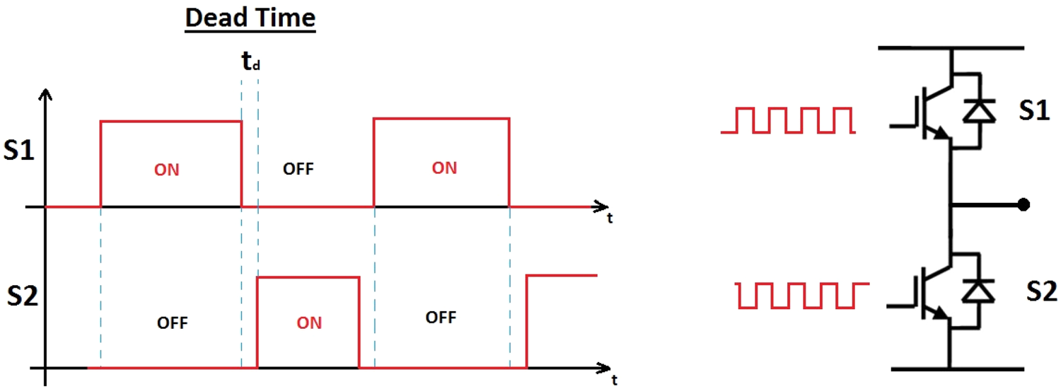
In a two-level three-phase inverter, the switching signals are generated by a Sinusoidal Pulse-Width Modulator (SPWM) in which the controller’s outputs are compared with a high frequency sawtooth carrier. The frequency of sawtooth carrier equals to the switching frequency of power switches which are MOSFETs or IGBTs. An SPWM’s output is high when its corresponding controller’s output is higher than the carrier. In this case, the upper switch in the corresponding inverter’s leg is ON and the lower switch is OFF. When the SPWM’s output is low, the upper switch is OFF and the lower switch is ON. Since real power switches are not able to be turned-on or turned-off instantly, in order to prevent the short-circuit in an inverter’s leg, a dead-time is implemented in the SPWM. It is defined as in Fig. 1. By implementing the dead-time, the turning-on command for one switch in a leg is started when enough time, i.e., ­td, elapsed from starting of the turning-off command of the other switch in the leg.

The inverter’s dead-time introduces low-order harmonics, i.e. the 5th, 7th, 11th, 13th, 17th, 19th,… har- monics, at the inverter’s output ­voltage8. At the result of the dead-time introduced harmonics, the inverter’s output current is heavily distorted. So, in an inverter’s operation, it is necessary to consider compensating for the dead-time effects.

In8 different strategies for mitigating the dead-time effects in power electronics converters are reviewed. They include pulse width adjustment, average voltage, current feedback, voltage feedback, and disturbance observer compensation methods. In the existing methods, in order to compensate for the dead-time effects, the robust stability of closed-loop control system is sacrificed. Therefore, there is the lack of a robust control technique for dead-time compensation in three-phase grid-tied inverters. The motivation of this paper is to compensate for the dead-time effects while the robust stability of closed-loop control system is maintained. For this purpose, in this paper, as the novel contribution, we propose an LQG-based multivariable control to compensate for the dead-time effects in three-phase grid-tied inverters. It employs the injected currents to grid feedback. No current direction detection circuit required, no feedforward terms employed, and no none-standard SPWM utilized in the proposed approach. We consider these as the advantages of the proposed approach over the existing methods.

The main features of proposed approach are as follows. • Besides the dead-time effects, it compensates for any low-order harmonics exists in the injected currents to grid originated from either the inverter, filter, or the grid.

• The closed-loop control system maintains the robust stability; meaning that it remains stable in spite of unmodelled dynamics and uncertainties.

Three‑Phase Grid‑Tied Inverter

A three-phase grid-tied inverter produces voltage harmonics at its outputs. In order to achieve sinusoidal current waveforms, the inverter’s outputs must pass through a filter. In Fig. 2, an LCL filter is employed for connecting the inverter to the grid at the PCC. The capacitor branch of the LCL filter provides a low impedance path for high- order harmonics. However, it shows high impedances at the fundamental frequency and low-order harmonics.

Figure 1.   Definition of dead-time in an inverter’s leg.

Www.Nature.Com/Scientificreports/

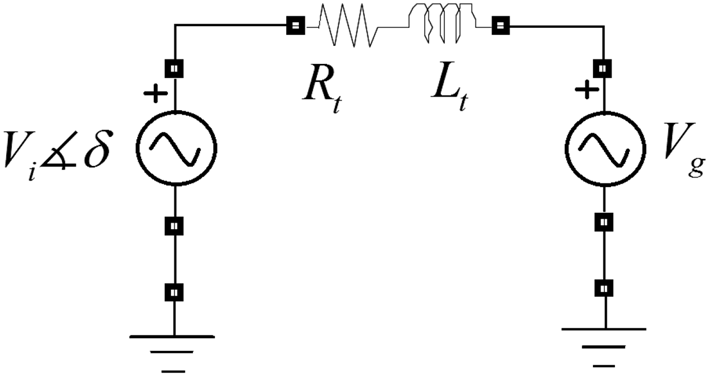
An equivalent-circuit for the three-phase grid-tied inverter at the fundamental frequency is shown in Fig. 3. In this figure, Vg is the grid’s voltage vector, Vi is the inverter’s voltage vector, Rt is the total resistance, and Lt is the total inductance exist between the inverter and the grid. It is the circuit representation of the grid-tied three-phase inverter’s vector model in a synchronous reference frame. In this representation, the d-axis of the synchronous reference frame is aligned with the grid’s voltage vector. Based on Fig. 3, by decomposing the vector equations into the real and imaginary parts, the following equations can be ­derived22.

where ωg is the grid’s angular frequency. By defining Ud = Vid −Vg and Uq = Viq , the above equations can be re-written in the standard state-space representation as follows. According to the above representation, it is clear that the grid-tied three-phase inverter is a MI–MO system with two inputs and two outputs. In fact, the vector

T Is The

output vector. One can derive the transfer matrix for the three-phase grid-tied inverter as follows. The above relation shows that the grid-tied three-phase inverter in the synchronous reference frame is a sec- ond-order system with two poles in the left half-plane. Also, it can be shown that the (Ap Bp) pair is controllable and the (Ap Cp) pair is observable and the plant is a minimum-phase one. Therefore, the three-phase grid-tied inverter has the required conditions to be controlled using the LQG multivariable ­controller27.

Grid

Figure 2.   Grid-tied inverter with LCL filter. Figure 3.   Circuit representation of grid-tied three-phase inverter’s vector model in a synchronous reference frame aligned with grid’s voltage vector.

Www.Nature.Com/Scientificreports/

Multivariable control systems analysis and LQG control design Multivariable control systems analysis. Figure 4 illustrates a general structure for a closed-loop control system where, R is the reference input, Y is the output, N is the measurement noise, ­Di is the plant’s input distur- bance, and ­Do is the plant’s output disturbance. In MI–MO systems, R and Y are two vectors of equal dimensions.

In addition to the closed-loop system stability, its performance must be desired in terms of the reference input tracking and noise and disturbance rejections. For a MI–MO system with n inputs and n outputs, the perfor- mance criteria can be stated as ­follows27.

(I + G(S)K(S))−1G(S)K(S)

R(s) , for ω ∈ωR , if G(s)K(s) >  > I is satisfied, then Y(s) ≈R(s) is achieved. ω ∈ωR means all the frequencies at which the elements of R(s) have significant energies.

Di(S) , For Ω ∈Ωdi , If G(S)K(S) >  > I And

K(s) >  > I are satisfied simultaneously, then Y(s) ≈0 is achieved. ω ∈ωDi means all the frequencies at which the elements of Di(s) have significant energies.

(I + G(S)K(S))−1

Do(s) , for ω ∈ωDo , if G(s)K(s) >  > I is satisfied, then Y(s) ≈0 is achieved. ω ∈ωDo means all the frequencies at which the elements of Do(s) have significant energies.

−(I + G(S)K(S))−1G(S)K(S)

N(s) , for ω ∈ωN , if G(s)K(s) <  < I is satisfied, then Y(s) ≈0 is achieved. ω ∈ωN means all the frequencies at which the elements of N(s) have significant energies. The reference inputs and input and output disturbances usually have most of their energies at low frequencies while most of the measurement noise’s energy is located at high frequencies. Based on the above, we can conclude that sufficient conditions for satisfying all of the closed-loop control system performance criteria are as ­follows27.

• At low frequencies: K(s) >  > I and G(s)K(s) >  > I are satisfied simultaneously. • At high frequencies: G(s)K(s) <  < I is satisfied. Singular value decomposition.

As can be seen in the above, we need to compare a given matrix with the identity matrix, i.e. I. To do so, the Singular Value Decomposition (SVD) technique is ­employed27. In the SVD, a given matrix A is decomposed into three matrices as follows. For Am×n , we have: where U is an m × m unitary matrix, i.e. UUT = I , and V is an n × n unitary matrix too, i.e. VVT = I . The is an m × n rectangular diagonal matrix with σi as the ith singular value of matrix A on the diagonal. We define σ as the largest singular value of A and σ as the smallest singular value of matrix A.

Based on the SVD technique, in order to satisfy the condition G(s)K(s) <  < I, it is sufficient that the condi- tion σ[G(s)K(s)] <  < 1 be satisfied. Also, to satisfy the condition G(s)K(s) >  > I, it is sufficient that the condition σ[G(s)K(s)] >  > 1 be satisfied.

LQG control design. The LQG consists of two optimal control problems including the LQR and the Kalman filter problems which the former is employed for the state feedback design and the latter is employed for the state ­estimation27. We consider the state-space representation of the plant as follows.

where Ap , Bp , Cp , and Dp are the plant’s state-space representation matrices. Also, w and v are assumed to be white noises which the former is considered as the process noise and the latter is considered to be the measurement noise. Their associated covariance matrices are shown as follows.

For the LQR, noises are not included in which we want to obtain an optimal gain for the full state variables feedback. The gain must minimize the following quadratic cost function.

Controller

Figure 4.   A generic closed-loop control system.

Www.Nature.Com/Scientificreports/

where R and Q are arbitrary positive-definite matrices. In LQR, we choose U = −KLQR X . It can be shown that

Klqr = R−1Bt

p PLQR where, PLQR is obtained from the Algebraic Riccati Equation (ARE) as follows. In the Kalman filter, noises are included in the plant’s model. The Kalman filter gain is chosen such that the following cost function in minimized.

where ˜X = ˆX −X is the state estimation error and ˆX is the estimation of state vector X . One can obtain the

Kalman Filter Gain As Kkalman = Pkalmanct

p G−1 where, PKalman is obtained from the following Filter Algebraic Riccati Equation (FARE). Based on the above, the multivariable LQG controller is composed as follows.

By employing the LQG controller, it can be shown that, the closed-loop system is stable for the nominal plant. It is also confirmed that the closed-loop control system with the LQG controller exhibits the robust ­stability27. However, its performance depends on the controller’s free parameters, i.e. KLQR and KKalman . We tune the free parameters such that the closed–loop control system performance is desired in terms of the reference inputs following and disturbances and noise rejections. In fact, to tune KLQR , we have to choose Q and R properly which are symmetric positive semi-definite and positive definite matrices, respectively. Also, to tune KKalman , the matrices N and G must be properly chosen.

The maximum and minimum singular values of the loop transfer matrix, i.e. G(s) K(s), as well as the controller, i.e. K(s), versus the frequency are employed for the designed controller’s evaluations. These diagrams are called the SVD diagrams. In fact, we select the KLQR and KKalman simultaneously. So, the impact of KLQR and KKalman , as a pair, is on the SVD diagrams. The SVD diagrams show the capability of designed controller in supressing the harmonics and in providing the robust stability. A higher SVD diagrams for the loop transfer matrix and for the controller in the low frequency range indicate a higher performance controller especially in terms of harmonics suppressions. Also, a lower SVD diagram for the loop transfer matrix in the high frequency range indicates a more robust controller.

Proposed Dead‑Time Compensation Method

The proposed method of this paper for dead-time compensation in three-phase grid-tied inverters is shown in Fig. 5. As shown, it employs the LQG multivariable control for regulating the injected currents to grid in the synchronous reference frame. To have the zero steady-state error in response to the step reference inputs, an integrator must be added at each of the plant’s inputs. Therefore, the yielding system under control is of the 4th order which is the order of the LQG controller too. In the other words, the order of the LQG controller equals to the order of the system under control.

Proposed method analysis. Besides the dead-time, the proposed method must deal well with harmonics in the grid’s voltages. In fact, both of the dead-time introduced harmonics and grid’s voltages harmonics are low- order harmonics. This is in contrast with the SPWM’s harmonics which are high-order ones. The SPWM’s har- monics are well suppressed by employing the LCL filter. So, in terms of the injected currents to grid, their effects can be ignored. The LCL filter behaves such as an L filter for low-order harmonics, since the capacitor branch can be considered as open-circuited at low frequencies. Since small inductors are utilized in the LCL filter, the resulting L filter at low frequencies is not able to significantly suppress the low-order harmonics. Therefore, this is the closed-loop control system’s responsibility to attenuate low-order harmonics as much as possible such that

+

Figure 5.   Proposed dead-time compensation method.

Www.Nature.Com/Scientificreports/

For a three-phase grid-tied inverter in the synchronous reference frame, low-order harmonics in the injected currents to grid result in disturbances in Id and Iq . As stated before, the inverter’s dead-time introduces the 5th, 7th, 11th, 13th, 17th, 19th,… harmonics at the inverter’s output voltage. Therefore, it introduces disturbances at 6ωg frequency and its multiples, i.e. 12ωg , 18ωg , …, in Id and Iq where, ωg is the grid’s angular frequency. In fact, the derived vector model for the three-phase grid-tied inverter described in "Three-phase grid-tied inverter" section is in the synchronous reference frame aligned with the grid’s voltage vector. In the case of an un-balanced grid, the reference frame is aligned with the positive-sequence voltage vector. The positive-sequence voltage vec- tor is rotating at ωg angular speed with respect to the stationary reference frame. Considering the 5th and 7th harmonics, the 5th harmonics produces a negative-sequence voltage vector rotating at − 5ωg angular speed with respect to the stationary reference frame. So, in the reference frame rotating at ωg angular speed, it is producing a 6ωg disturbance. On the other hand, the 7th harmonics produces a positive-sequence voltage vector rotating at 7ωg angular speed with respect to the stationary reference frame. So, in the reference frame rotating at ωg angular speed, the 7th harmonics produces a 6ωg disturbance too. Therefore, the 6ωg disturbance in the synchronous reference frame is at the result of both the 5th and 7th dead-time introduced harmonics. Note that, the amplitudes of disturbances are proportional to the amounts of dead-time considered. Also, they are inversely proportional to the frequency of the disturbance.

An un-balanced grid introduces disturbances at 2ωg frequency in Id and Iq which are the effects of the negative-sequence component exists in an un-balanced grid. It is, therefore, clear that the inverter’s dead-time introduces disturbances with the highest frequencies in Id and Iq . So, they are the most important disturbances in an inverter’s operation.

Proposed method design. We define G(s) = Gp(s)Ga(s) as the new plant where, Ga(s) is the transfer matrix of the two augmented integrators at the plant’s inputs. The LQG MBC is composed according to the equation in (13) and the procedure described for choosing its free parameters, i.e. KLQR and KKalman . We design the LQG controller such that G(s)K(s) >  > I and K(s) >  > I are satisfied simultaneously for the low frequency range up to the 6ωg frequency. Note that, the 6ωg frequency is the first dead-time introduced disturbance and it has the highest amplitude. This guarantees appropriate reference inputs tracking and disturbance rejection. It, of course, covers the 2ωg frequency disturbance too which is the un-balanced grid introduced disturbance.

An experimental set-up, as shown in the Online Appendix, is manufactured for the purposes of implement- ing and verifying the proposed method. In Table 1, its parameters are listed. A three-phase BSM50GP120 IGBT module is employed in the experimental set-up. We considered the switching frequency of fs = 20 kHz for the IGBT power switches. An LCL filter with the parameters listed in Table 1 is designed to suppress the SPWM’s harmonics. The inverter side inductor, Li, and the grid side inductor, Lg, are wound on two separate toroidal cores for which the windings’ resistances are measured. The Lt = Li + Lg and Rt is the summation of the inverter side and grid side inductors’ windings resistances.

According to the turn-on and turn-off times of the IGBT power switches as well as the IGBT’s driver IC, a dead-time equals to td = 1.5 µs is calculated which guarantees that no short-circuit occurs in an inverter’s leg. Note that, in order to minimize its adverse effects, the dead-time calculated is the minimum possible one. It is implemented in a three-phase SPWM to command the three legs of inverter. For the given new plant, the LQG controller is designed and the results are shown in Fig. 6. In Fig. 6, the SVD diagrams are shown both for the loop transfer matrix, i.e. G(s)K(s), and the LQG controller, i.e. K(s). For the purpose of comparison, the results for a multivariable PI controller as presented ­in28 are shown too.

As stated before, to have the desired performance, it is sufficient to have σ >  > 1 in the low frequency range up to the 6ωg frequency both for the loop transfer matrix and the controller. Also, for the frequency range above the switching angular frequency, i.e. ωs, it is sufficient to have σ <  < 1 for the loop transfer matrix. Note that, we considered the frequency range above the switching angular frequency as the high frequency range in this study.

Table 1.   Parameters of the manufactured experimental set-up for three-phase grid-tied inverter.

0.2 Mh

Summation of resistances of inverter side and grid side inductances

Deployment In Out-Of-Position Situations

D. Bendjaballah1, A. Bouchoucha1, M. L. Sahli1,2* and J-C. Gelin2

Abstract

Side-impact collisions represent the second greatest cause of fatality in motor vehicle accidents. Side-impact airbags have been installed in recent model year vehicle due to its effectiveness in reducing passengers’ injuries and fatality rates. In meeting these requirements, simulations of folding and deploying airbags are very useful and are widely used. The paper presents a simulation method for the deploying airbags using three materials in different working conditions. Finite element analysis is primarily used to evaluate this concept. In these simulations, the gas flow is described by the conservation laws of mass, momentum, and energy. The numerical results indicate that the FE method in this paper is capable of capturing airbag deploying process accurately.

Keywords: Airbag simulations, Out-of-position, Crash, Modeling, Out-of-position

Background

The passive safety of cars has become a very high prior- ity issue for the automotive industry. Today, there are not only one or two airbags in a car; certain models have ten times more than that. With the increasing usage of airbags, the number of accidents where the airbag itself can cause an injury to the occupant also increases

(Augenstein Et Al. 2003; Gabauer And Gabler 2010;

Audrey et al. 2011). As is well known, safety belts are also now devices designed to provide protection to the users of vehicles during crash events, minimizing the loads necessary to adapt their movement to the move- ment of the car (Freesmeier and Butler 1999; Schmitt et al. 1997). In general, the seat belt is designed to restrain the occupant in the vehicle and prevent the

Occupant From Having Harsh Contacts With Interior

surfaces of the vehicles. The airbag acts to cushion any impact with vehicle structure and has positive internal pressure, which can exert distributed restraining forces over the head and face. As a safety component of auto- mobile, an airbag decreases occupants’ injury likelihood effectively in case of an accident (Ruff et al. 2007). These safety elements can reduce the death rates on the roads, and its protection effects have been widely approved (Crandall et al. 2001; Teru and Ishikawa 2003). With computational tools such as finite element methods designed for dynamic contact problems, crashworthiness simulations can now be used with reliable accuracy to evaluate occupant protection in various collision condi- tions with safety metric/parameters such as acceleration, head injury criteria, intrusion distance, intrusion vel- ocity, and neck forces (neck injury risk or whiplash).

Thus, new types of airbag products are being developed to handle different collision scenarios.

Become Standard Equipment On Most New Passenger

vehicles (Braver and Kyrychenko 2004; Teng et al. 2007; Yoganandan et al. 2007). The airbag cushion is com- posed of a woven fabric which is rapidly inflated during a car crash. The airbag dissipates the passenger’s kinetic energy thereby reducing injury through biaxial stretching of the fabric bag and escaping gas through vents. There- fore, the performance of the airbag is greatly influenced by the mechanical properties of the fabric. Generally, air bags are designed to deploy in a crash that is equivalent to a vehicle crashing into a solid wall at 8 to 14 mph.

Air bags most often deploy when a vehicle collides with another vehicle or with a solid object like a tree. There are various types of airbags: frontal, side-impact, and curtain airbags. In general, the passenger side airbags are usually larger than the driver airbags (see Fig. 1).

Besançon, France

© The Author(s). 2017 Open Access This article is distributed under the terms of the Creative Commons Attribution 4.0 International License (http://creativecommons.org/licenses/by/4.0/), which permits unrestricted use, distribution, and reproduction in any medium, provided you give appropriate credit to the original author(s) and the source, provide a link to the Creative Commons license, and indicate if changes were made.

Bendjaballah et al. International Journal of Mechanical

Doi 10.1186/S40712-016-0070-2

Extensive studies have shown that the airbag deploy- ment in load cases consists of two occupant loading phases: a punch-out effect where the airbag bursts out of its container with the airbag and airbag module cover accelerating towards the occupant and a second loading phase during which the airbag is taking on its deployed shape and volume (membrane-loading effect). Bankdak et al. (2002) developed an experimental airbag test system to study airbag-occupant interactions during close proximity deployment. The results provided insight for simulating the effect of inflation energy and mass flow on target response. Bedard et al. (2002) found that while left-side (driver-side) impacts accounted for only 13.5% of all crashes, the fatality rate among these

Crashes Was 68.3% In Comparison To Front Impact

(48.3%), right-side impact (31.3%), and rear impact (38.4%). These studies underscore the importance of oc- cupant safety during side-impact collisions. In the last years, the current market requested to reduce the time and cost airbag development. In order to achieve this result, virtual simulations play an important role since they allow to minimize the number of experimental tests (Pei et al. 2013; Cao et al. 2014). Several simulation models of airbag were established (Wang et al. 2007). It is feasible to optimize the parameters of airbag deploy- ment using simulation technology. Experimental and numerical studies have quantified injury risks to close- proximity occupants from deploying side airbags. These studies have focused on the prevention of the most ad- verse effects of airbag deployment (Duma et al. 2003).

Other studies have proposed airbag characteristics to minimize particular biomechanical responses (Haland and Pipkorn 1996). In a more recent study, Marklund and Nilsson (2003) compared deformation patterns with experimental data as well as the computational costs associated with three different airbag deployment simu- lation methods; they concluded that the SPH method is relatively inexpensive and produces incremental deform- ation patterns that compare most closely to the experi- mental results. The process of inflation of an airbag is one of the determining factors in saving lives. The duration from the initial impact of the crash to the full inflation of an airbag is about 40 ms, and during this time, the airbag goes from being in a folded state to a fully inflated state, with a high internal pressure. After achieving this state, the airbag begins to deflate, thus providing a nice cushion for the body impacting it.

Ideally, the person in the crash should come into contact with the airbag at this time. In the present study, a large volume passenger side airbag model is developed to handle different collision scenarios. The main aim is evaluate the performance of deploying of passenger side airbag using finite element methods (FEM).

Materials

The tensile specimens were made in different airbags (P: Peugeot, R: Renault, and VW: Volkswagen) with a length of 200 mm long and a width of 40 mm. Table 1 shows the mechanical properties of the airbag.

Tensile Tests

To determine the mechanical properties of the material of airbag used in the test pieces, tensile tests were performed on Lloyd EZ20 universal testing machine in Constantine. These tests were conducted using rect- angular samples. The axial force and axial displacement acquired during a test are converted into stress and the strain in order to be used for the fabric material model.

The continuous recording of the stress-strain data was performed during both the load and unload phases. A minimum of five samples were made in order to check the repeatability of the measurements. All the data was collected by using a PC-based data acquisition system and analyzed by commercial software. The picture frame test device that is made for this study is shown in Fig. 2.

Fig. 1 a Frontal and side airbags. b Oblique view of facet occupant model in sitting posture following airbag deployment (Lim et al. 2014)

0.150

Bendjaballah et al. International Journal of Mechanical and Materials Engineering (2017) 12:12

Page 2 Of 9

Figure 3 shows the stress-strain relationship of the airbag sample under axial tensile loads. The results are showing a linear increase in extension with the increas- ing stresses. This is an expected output and it confirms with the theoretical behavior of a sample subjected to tensile stress. The rupture strain values for different airbags (R/P/VW) were 0.322, 0.441, and 0.472, respect- ively. The measured elastic parameters (i.e., Young’s modulus E and initial yield strength) and Poisson’s ratio are summarized in Table 2. The tensile tests of the woven fabrics can show differences on mechanical prop- erties because woven fabrics can resist in-plane shear loads once the yarn lock-up angle has been reached. The differences of material property on material direction can affect the shape of fully deployed bag (see Fig. 3b).

Theoretical Background

Numerical simulations of airbags use very complex and techniques such as an orthotropic model to identify the mechanical behaviors during the airbag inflation and the fluid mechanics (gas flow) to describe the inflator gas flow (pressure gradient) and improve the representation of the pressures within the airbag. To model the airbag as an orthotropic model, three material constants have to be provided. Assuming a plane stress condition, the

Ð1Þ

where σ is the normal stress and τ is the shear stress, the subscript refers to the principal material directions, i.e., the fill and warp directions. Also, ε and γ are the strain components. The material elastic constants Qij are

Ð2Þ

where E1 and E2 are the Young’s modulus in the fill and wrap directions and G12 is the shear modulus of the fabric material. νij is the Poisson ratio of the material.

The gas exerts a pressure load on the airbag causing it to expand. This expansion puts the airbag under tensile stress lowering the expansion rate. In this study, heat conduction and heat transfer is not taken into account.

Fig. 2 A photograph of Lloyd EZ20 universal testing Fig. 3 Stress versus strain using Lloyd EZ20 machine for a three different airbags at 0° and 90° and b VW airbag test specimens at

Different Angles

Table 2 Physical and mechanical properties of the airbag

Page 3 Of 9

In the deployment of an airbag, an inflator supplies high velocity gas into an airbag causing it to expand rapidly. The gas inside the airbag is assumed to be ideal, to be of constant entropy, and to satisfy the equation of state:

Ð3Þ

Here p, ρ, and e are respectively the pressure, density, and specific internal energy, and γ is the ratio of the heat capacities of the gas. The gas flow is described by the conservation laws for mass, momentum, and energy that

Ð4Þ

here, V is a volume, A is the boundary of this volume,

N Is The Normal Vector Along The Surface A, And U

denotes the velocity vector in the volume. Applying Bernoulli’s equation in the case of an ideal gas with

Ð5Þ

Here, the subscript ex denotes quantities at the throat of the tube. Furthermore u, p, and ρ denote the quan- tities inside that part of the tube that is supplying mass.

Materials And Boundary Conditions

The airbag system mainly consists of three parts: the airbag itself, the inflator unit, and the crash sensor or diagnostic unit. Thus, to study the behavior of the airbag using FE simulations, we need to have an FE model of the airbag in the folded position. A FE model of the airbag was used to simulate the test condition as shown in Fig. 5. LS-DYNA® material model FABRIC (MAT_34) is used to simulate the airbag material. It is a variation of the layered orthotropic material model. Additionally, in the LS-DYNA® material model, fabric leakage can be accounted for. However, for this CAB material, the leak- age is almost negligible and therefore no leakage is specified. The mechanical properties can be determined from the physical test. Typical material properties for airbag fabrics are taken as given in Chawla et al. (2004a) (Table 3). These properties are used to simulate inflation process of airbag (see Table 1). The car dashboard is modeled as the rectangular thin plate using a MAT_RI-

Gid Material, And The Degrees Of Freedom Are Con-

strained in all the directions. The similar properties of thermoplastic polymer are assigned for contact purposes. The porosity of the fabric is assumed zero. The nitro- gen gas is taken for inflating the airbag. Properties of nitrogen gas and initial bag conditions are shown in Table 4. The example on which we perform the study is a typical passenger side airbag. The geometric de- tails have been measured from a commercially avail- able airbag. The initial state of the airbag is a closed rectangular whose sides are to be finished to 482 × 635 mm2 and is shown in Fig. 4.

Table 3 Material properties of airbag and rigid plate used in FE

–

Table 4 Initial values used for FE simulation of the swelling of

3.33 × 10−4

Fig. 4 The initial airbag geometry in the form of a rectangular Bendjaballah et al. International Journal of Mechanical and Materials Engineering (2017) 12:12

Related Journal Articles & DOI Links

Selected peer-reviewed publications relevant to 12 Lead ECG Acquisition. Click the DOI to access the full paper (may require institutional access).

Why Choose Us?

Bangalore guidance for robotics, Spectre and autonomous systems projects.