Inductive Power Transfer Ipt Matlab

Inductive Power Transfer (Ipt) System

Jr-Uei William Hsu, Aiguo Patrick Hu and Akshya Swain

1. Introduction

Inductive Power Transfer (IPT) systems have successfully been developed and used to replace traditional conductive power transfer systems where physical connection is either inconvenient or impossible, such as biomedical implants, undersea vehicles, and contactless battery chargers of robots, for providing power to movable or detachable loads (Kim et al., 2001; Feezor et al., 2001; Harrison, 2007). As IPT systems extend to more fields, better control methods are required to cope with various operating environments to satisfy users’ needs.

Difficulties in controlling the power flow in a wireless/contactless power pickup using IPT technologies can arise from several factors, which include but not limited to load and circuit parameter variations, magnetic field coupling variations between the primary and secondary coils, the operating frequency drift of the primary power supply, etc (Jackson et al., 2000; Chao et al., 2007). These factors can cause the output voltage of the secondary power pickup to deviate significantly from the original designed value, resulting in an undesirable characteristic for applications where a stable output voltage is required. Hence, there is a need to develop controllers under various operating conditions.

Practical power flow control of an IPT sytem can generally be categorized into three different types: namely, primary power supply control, secondary power pick-up control, and coordinated control of both primary and secondary circuits. Among these three, direct power flow control at secondary power pickups is most commonly used to stabilize the output voltage, paricularly for multiple power pickup applications (Hu et al., 2007; Wang et al., 2006; Gao, 2005). This chapter presents the basic theory and control algotithm of an improved directional tuning control method for power flow control of secondary contactless/wireless power pickup circuits.

2. Background of Inductive Power Transfer (IPT) system The basic structure of an IPT system is shown in Fig. 1 (Wang et al., 2000; Wang et al., 2005; Bieler et al., 2002). The system comprises two electrically isolated parts: the primay power supply and the secondary power pickup. The primary power supply is normally stationay and consists of a resonant power supply and an elongated conductive path for producing a constant AC track current. The secondary movable part, also called the power pickup, is mutually coupled with the primary track and moves with respect to the track loop as the Source: Advances in Solid State Circuits Technologies, Book edited by: Paul K. Chu,

222

operation requires. Since the system is often loosely coupled between its primary and secondary side, the induced voltage source is usually unsuitable for direct use in applications. As a result, proper tuning and control are essential in the system design for providing a constant DC voltage to the load.

Input

Fig. 1. Basic structure of an IPT system with uncontrolled power pickup. Figure 2. shows the structure of a typical IPT power pickup. LS and CS represent the secondary pickup coil inductance and tuning capacitance respectively, a parallel tuning configuration is adopted here for boosting the induced open circuit voltage.

M

Fig. 2. Basic structure of an IPT power pickup with shorting-control. The open circuit voltage VOC and short circuit current (ISC) of the pickup coil are governed

(2)

In Figure 2 the voltage VAC after tuning is converted from AC to DC through rectifiers to provide a DC output voltage VOUT. To simply the analysis, the rectifier and load can be represented with the equivalent AC resistor RAC. The transfer function of the system given in (3) can be derived from the simplified second order system shown in Fig. 3, and it also can be seen that at steady state the pickup provides a current source to the load when it is fully-tuned.

Www.Intechopen.Com

Directional Tuning Control of Wireless/Contactless Power Pickup

Vac

Fig. 3. Simplified second order tuning circuit of power pickup.

(3)

where ω is the system operating frequency. The maximum voltage boost-up factor of power pickup is gorverned by Q factor of the tuning circuit, and under fully-tuned condition it can

(5)

The AC equivalent load resistance RAC is given by:

(6)

where RLoad is the DC load resistance. A DC inductor LDC is normally added after the rectifier to maintain a continuous current flow, so that the available power of the secondary pickup can be fully delivered to the load. The output voltage regulation is normally achieved by using a well-known control technique called “Shorting-Control“ (Boys et al., 2000; Elliot et al., 1995; Raabe et al., 2007). Its working principle is similar to a boost converter. The constant output voltage is maintained by controlling the average current flowing through the load by switching a semiconductor device (S, shown in Fig. 2) on and off using either hysteresis or PWM control. However, this controller cannot maintain the full-tuning condition of the secondary power pickup circuit. Therefore, the maximum power which can be transferred may be significantly reduced if the circuit parameters vary. And due to the fact that the short circuit current of the pickup coil has to flow through the switch during shorting period, which causes high power losses particularly under light loading conditions, this shortcoming also decreases the potential capability of the primary power supply to operate with more pickups due to unnecessary power loss and possible circuit mistuning.

An alternative method that has been investigated to further improve the power flow control is the dynamic tuning/detuning technique (Hu et al., 2004; Si et al., 2006). Figure 4 shows the general structure of dynamic tuning/detuning control scheme. The fundamental concept of this control method is to dynamically change the tuning condition of the power pickup according to the actual load demands. This helps to maintain maximum power transfer

M

Fig. 4. Basic structure of an IPT power pickup with dynamic tuning/detuning control. capacity, improve the overall efficiency of the system under light loading condition while keeping the output voltage to be constant. The control strategy is achieved by using a PI controller to control the on/off time of a soft-switched tuning inductor/capacitor to obtain the desired values of equivalent inductance/capacitance in the resonant tank. However, because the relationship between the tuning components and the output voltage is bell- shaped (shown in Fig. 5), there are two possible operating points with one in the over-tuned region and the other in under-tuned region. If the operating point has been accidentally shifted to the other region due to variations of circuit parameters, the desired equivalent values may be tracked in the wrong direction and consequently fail to control the output voltage.

To overcome the problems associated with existing control methods of power pickups such as shorting control, dynamic tuning/detuning control, etc., an LCL (Inductor-Capacitor- Inductor) based power pickup with directional tuning control (DTC) algorithm is proposed and has been discussed in detail in this chapter. Its working principle is similar to the dynamic tuning/detuning control technique. However, instead of using the traditional PI controller to perform the tracking process, it uses the present and previous control results to determine the correct tracking direction in the next step, and retune the circuit to deliver the required power (Hsu et al., 2006). Such an approach covers the full-tuning curve, so dual- side (full-range) control can be achieved. The proposed controller can provide reliable

Resonance Point

Fig. 5. Relationship between tuning inductance/capacitance and output voltage of IPT power pickup.

225

constant output voltage under various circuit parameter variations, thus eliminating the need for tedious fine-tuning process required by traditional IPT pickups. As a result, it is more cost-effective for mass production with reduced tuning and component tolerance requirements.

3. Effects of power pickup parameter variations on output voltage In practical operations, the pickups are often deviated from its designated operating point due to the variation of circuit parameters. Since the deviation of output voltage may not be regulated by the general controller, especially under full-tuning range, the effect of each parameter variation on the output voltage is therefore need to be individually examined so the control range based on the given maximum tolerance to pickup parameters can be better understood (Hsu et al., 2007). The considered circuit parameters include: system operating frequency, magnetic coupling between the primary and secondary side, load resistance and tuning capacitance. Figure 6 shows the structure of the proposed secondary power pickup.

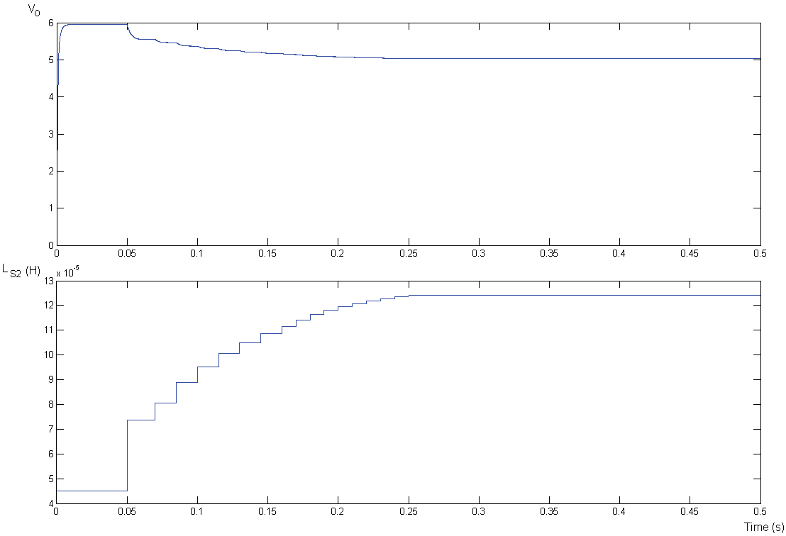
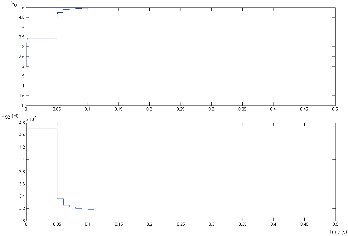
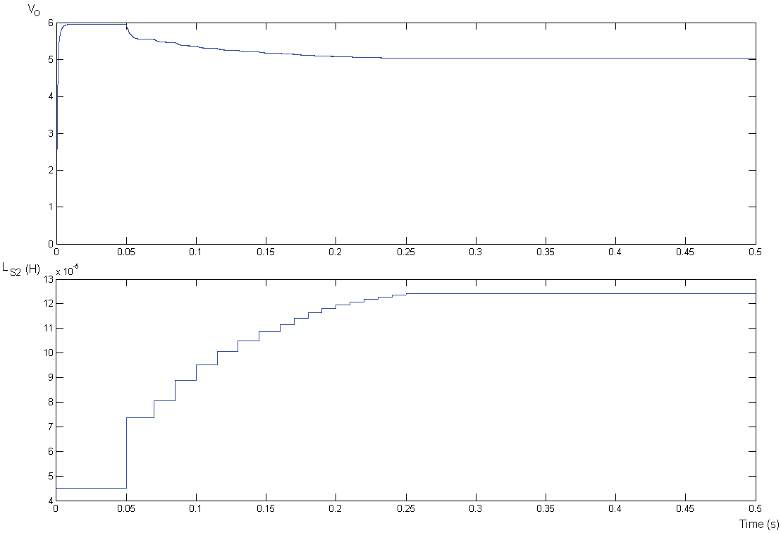
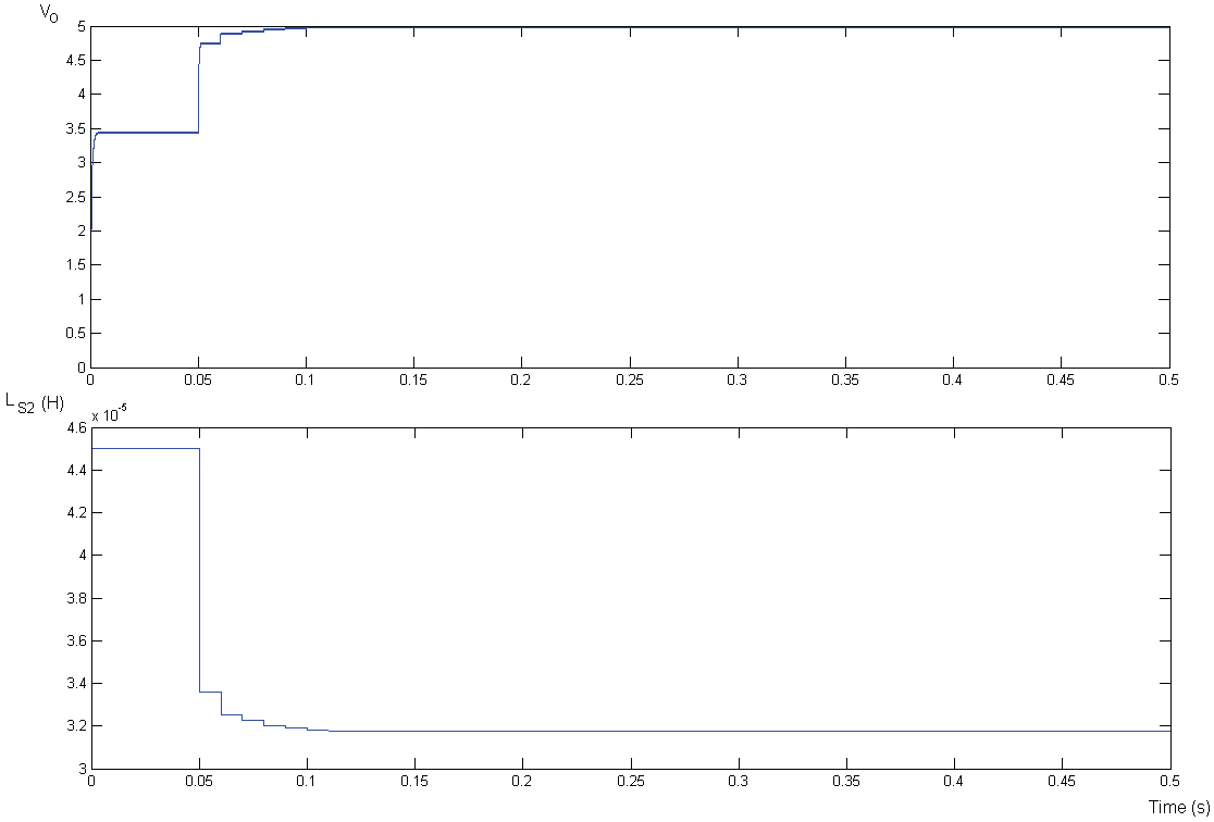
An LCL tuning configuration is being used here to provide a constant output voltage to the load under resonant conditions, and a magnetic amplifier in the tuning circuit serves as a variable inductor for changing the tuning condition of the power pickup. The DC current (IMA) which controls the magnetic amplifier is varied through a transistor operating in linear mode which essentially functions as a variable resistor. The equivalent inductance of LS2 is adjusted through changing the output signal Vctrl from the DTC algorithm, which allows the power pickup to deliver the right amount of power required by the load (Hsu et al., 2009).

M

Fig. 6. The proposed LCL power pickup with directional tuning control. The boost-up factors for ac voltage (VAC) and current (IAC) of the LCL tuning circuit can be determined from the following two transfer functions.

(8)

As shown in Fig. 6, the value of CST can be separated into CS1 and CS2 which resonate respectively with LS1 and LS2 i.e. jωLS1CS1= jωLS2CS2=1. The ac voltage boost-up factor kr under full resonant condition can be expressed as:

(9)

With the considered circuit parameters, the magnitude of AC boost-up factor kv in (7) can be

(10)

where αv, αr, αf, and αc is the per unit variation of open circuit voltage, load resistance, primary operating frequency, and tuning capacitance, respectively and these are equal to unity when they are at their nominal values. For example if the open circuit voltage increases or decreases by 10%, the value of αv is set to 1.1 or 0.9 respectively. By rearranging (10) into a quadratic equation of LS2, the solution can be obtained as:

(8)

where kmin is defined as the required minimum ratio between VAC and VOC, reflecting the required AC voltage boost-up capability under all possible variations in αv, αr, αf, and αc.

3.1 System Operating Frequency Variation

Depending on the design of primary power supplies, the operating frequency may drift which often causes significant power loss due to the mismatch in the resonant frequency between the primary and secondary sides. This is particularly a major concern in wireless power transfer systems using resonant variable frequency converters.

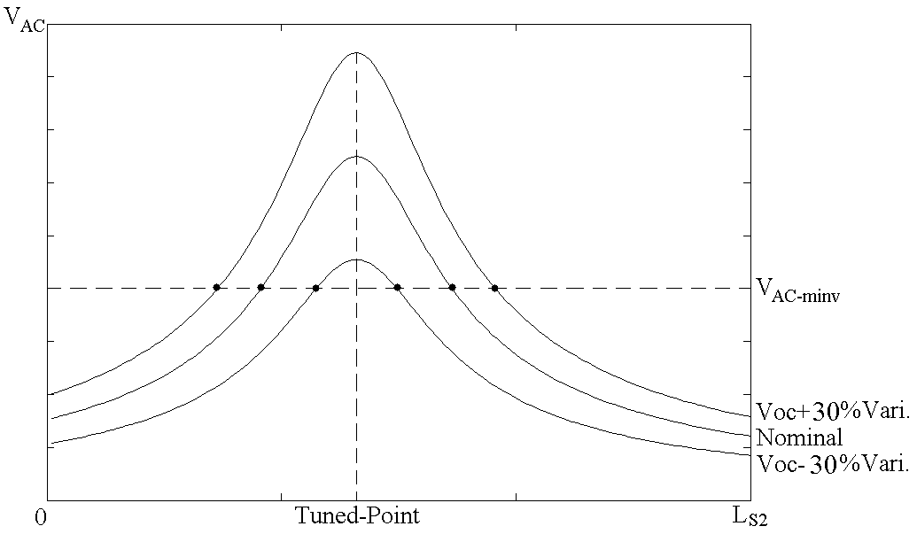
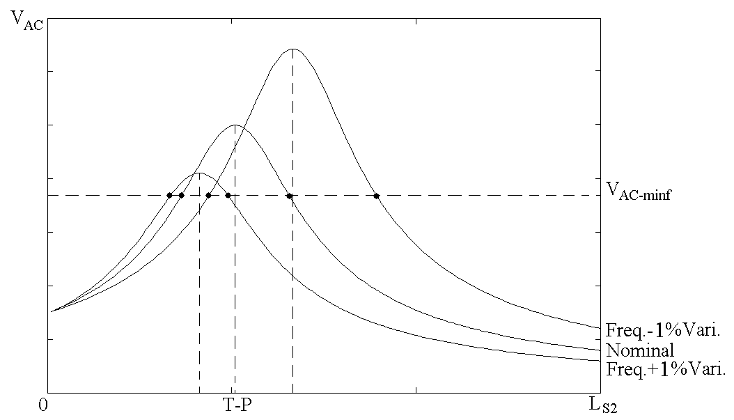
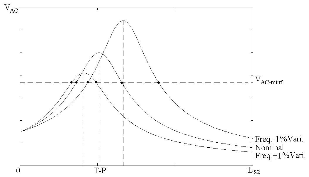
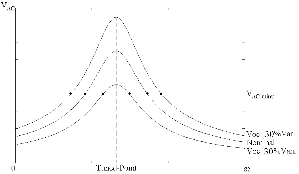
Figure 7 shows the effects of system operating frequency variation on AC voltage of the power pickup. It can be seen from the graph that the operating frequency is drifted with the variation so the tuned-point (T-P) is shifted accordingly. As for the magnitude of VAC, it is also changed due to the tuning circuit requires different value of LS2 to achieve resonant condition and therefore resulted in various kr. Note that there are two possible operating points for LS2 to compensate for the variations, and both of them are able to keep VAC constant. However, depending on the design specifications, designer can choose to either work with the lower or higher inductance point.

227

Fig. 7. The effect of system operating frequency variation on AC voltage of LCL power pickup.

3.2 Magnetic Field Coupling Variation

The IPT system is normally involved in loosely coupled applications which allow free movements between the primary and secondary sides. In such applications, fluctuating open circuit voltage of the pickup coil is usually caused by coupling variations due to the free movements, and hence it needs to be compensated for keeping the output voltage constant.

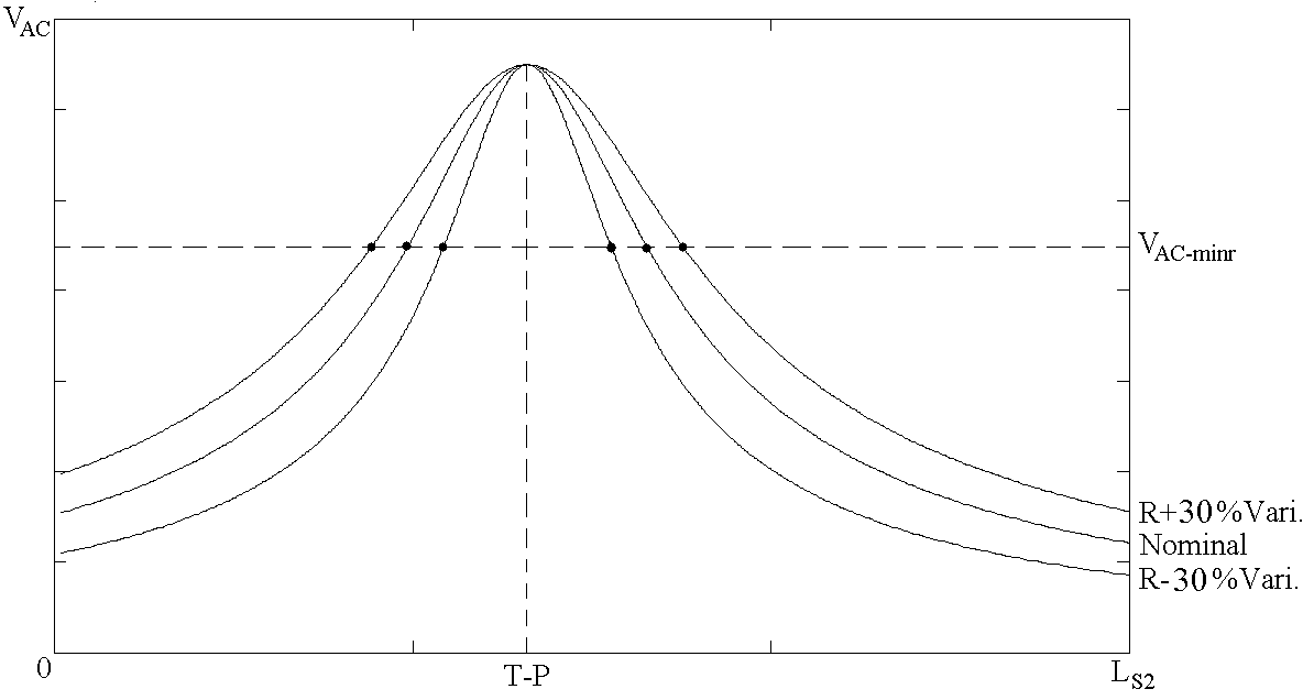
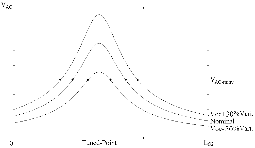
Effect of the magnetic field coupling variation on AC voltage of the power pickup is shown in Fig. 8. It can be seen that the tuned-point and shape of the tuning circuit have both remained the same. Only the magnitude of open circuit voltage of the pickup coil has been changed and therefore resulted in different peak value of VAC.

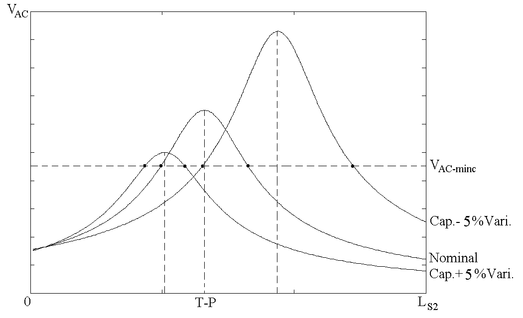
Fig. 8. The effect of magnetic coupling variation on AC voltage of LCL power pickup.

3.3 Load Resistance Variation

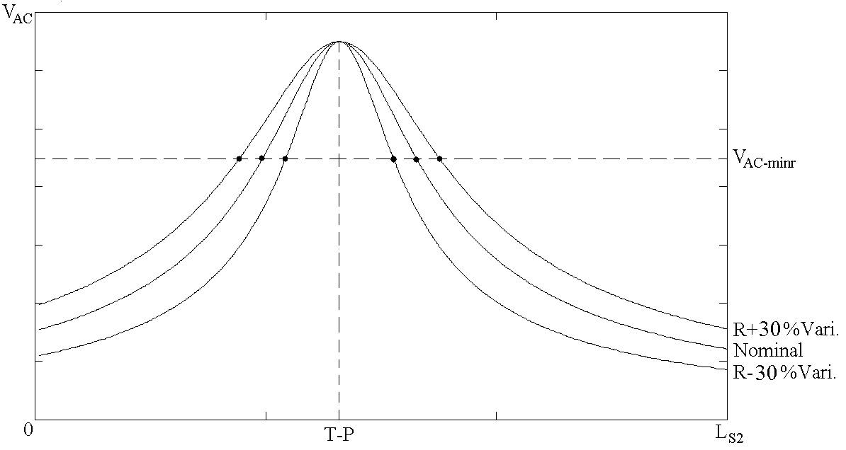
Fig. 9. The effect of load resistance variation on AC voltage of LCL power pickup. Another variable whose effects need to be studied is the load resistance which varies as the loading condition changes. 9 shows the effect of load variation on VAC. It can be seen from Fig. 9 that when the load increases, the sensitivity of VAC with respect to LS2 decreases.

On the contrary, when the load decreases, VAC becomes very sensitive to the change of LS2. These two results have indicated that when the power pickup is operating at extreme loading conditions, either LS2 will not be able to compensate for the variation, or the tuning circuit will be too sensitive with respect to LS2.

3.4 Tuning Capacitance Variation

Unwanted variations of the tuning capacitor such as the variation caused by temperature change may result in undesired tuning condition change and affect the output voltage. This is particularly severe when the seondary system is working with high Q factor since the circuit becomes extremely sensitive to parameter variations.

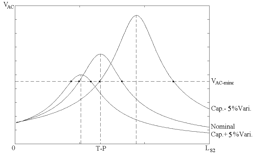
Similar to the operating frequency variation, both the magnitude of peak VAC and the T-P have been changed and shifted to different places after the variation as can be seen from Fig. 10. Note that as the tuning capacitance decreases/increases, the corresponding LS2 also needs to be increased/decreased to keep the circuit tuned, and this consequently causes the pickup to have different peak VAC (or kr).

3.5 Determination of range of the tuning inductance In practical operations, the system operating frequency, magnetic coupling, and load resistance as well as other parameters may vary simultaneously. To design the variable capacitor and its controller properly, the worst-case maximum and minimum values of LS2 should be identified based on the integrated effect of concerned parameter variations to cover the full control range. Given the maximum allowed tolerance for each variation, the desired maximum and minimum inductance can be calculated by using (8), with the

229

Fig. 10. The effect of tuning capacitor variation on ac voltage of power pick-up. 1.

•

Open circuit voltage, operating frequency, tuning capacitor, and load resistance are all at Nominal value - maximum allowed tolerance. 2.

•

Open circuit voltage, operating frequency, tuning capacitor, and load resistance are all at Nominal value + maximum allowed tolerance. The method presented here can be extended to other possible parameter variations in the system for calculating the range of LS2 in worst-case scenario.

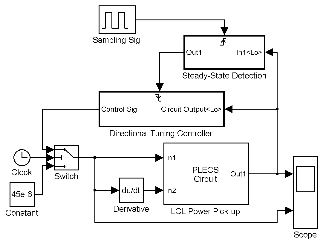
4. Design of Directional Tuning Control (DTC) algorithm In both the shorting-control and dynamic tuning/detuning control method, traditional PI controller has been employed for their output voltage regulation and proven to be effective when the power pickup operates under single-side tuning condition. Nevertheless, it is practically difficult to maintain single-side operation, particularly for high Q systems. The system parameter variations may force the pickup to traverse from one operating region to the other region of the tuning curve and fail to control the output voltage. Directional Tuning Control (DTC) algorithm has been proposed to overcome the problems associated with full-range tuning of the power pickup. The fundamental concept of DTC is based on comparing the present value of control input with its immediate past value, and then use this result to determine the next control action. Instead of depending only on the output error detection as the traditional controllers do, the proposed controller generates the control signal based on the memory of previous control action following the procedure outlined in the flow chart of Fig. 11.

4.1 Standard Procedure Of Dtc Algorithm

The flow chart of DTC algorithm is shown in Fig. 11. Standard procedures of the DTC algorithm start with initializations. In this process, the controller initializes the settings

230

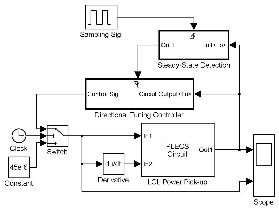
according to the user specifications, which include sampling time of the controller and initial state of each processing block. Since the algorithm is designed for controlling the power pick-up to focus on the steady state control, variation of the circuit time constant caused by other system parameter variations must be specified in the initial time delay of the program to avoid inaccurate sampling. After the initialisations, the output voltage at present-state VOUTk will be sampled, stored, and used to compare with a voltage reference Vref and its previous stored value VOUTk-1 for generating logic signals S1(k) and S2(k), respectively. These control signals are then collected by the next processing block to check with a predetermined truth table (Table 1) for determining the next-state control signal S4(k).

Note that the memory block after the decision block stores the present control signal as S3(k), so it can later be used in the next execution for validity checking of the present control action.

S1(K) = 0

Fig. 11. Flow chart of the directional tuning control algorithm.

Deployment In Out-Of-Position Situations

D. Bendjaballah1, A. Bouchoucha1, M. L. Sahli1,2* and J-C. Gelin2

Abstract

Side-impact collisions represent the second greatest cause of fatality in motor vehicle accidents. Side-impact airbags have been installed in recent model year vehicle due to its effectiveness in reducing passengers’ injuries and fatality rates. In meeting these requirements, simulations of folding and deploying airbags are very useful and are widely used. The paper presents a simulation method for the deploying airbags using three materials in different working conditions. Finite element analysis is primarily used to evaluate this concept. In these simulations, the gas flow is described by the conservation laws of mass, momentum, and energy. The numerical results indicate that the FE method in this paper is capable of capturing airbag deploying process accurately.

Keywords: Airbag simulations, Out-of-position, Crash, Modeling, Out-of-position

Background

The passive safety of cars has become a very high prior- ity issue for the automotive industry. Today, there are not only one or two airbags in a car; certain models have ten times more than that. With the increasing usage of airbags, the number of accidents where the airbag itself can cause an injury to the occupant also increases

(Augenstein Et Al. 2003; Gabauer And Gabler 2010;

Audrey et al. 2011). As is well known, safety belts are also now devices designed to provide protection to the users of vehicles during crash events, minimizing the loads necessary to adapt their movement to the move- ment of the car (Freesmeier and Butler 1999; Schmitt et al. 1997). In general, the seat belt is designed to restrain the occupant in the vehicle and prevent the

Occupant From Having Harsh Contacts With Interior

surfaces of the vehicles. The airbag acts to cushion any impact with vehicle structure and has positive internal pressure, which can exert distributed restraining forces over the head and face. As a safety component of auto- mobile, an airbag decreases occupants’ injury likelihood effectively in case of an accident (Ruff et al. 2007). These safety elements can reduce the death rates on the roads, and its protection effects have been widely approved (Crandall et al. 2001; Teru and Ishikawa 2003). With computational tools such as finite element methods designed for dynamic contact problems, crashworthiness simulations can now be used with reliable accuracy to evaluate occupant protection in various collision condi- tions with safety metric/parameters such as acceleration, head injury criteria, intrusion distance, intrusion vel- ocity, and neck forces (neck injury risk or whiplash).

Thus, new types of airbag products are being developed to handle different collision scenarios.

Become Standard Equipment On Most New Passenger

vehicles (Braver and Kyrychenko 2004; Teng et al. 2007; Yoganandan et al. 2007). The airbag cushion is com- posed of a woven fabric which is rapidly inflated during a car crash. The airbag dissipates the passenger’s kinetic energy thereby reducing injury through biaxial stretching of the fabric bag and escaping gas through vents. There- fore, the performance of the airbag is greatly influenced by the mechanical properties of the fabric. Generally, air bags are designed to deploy in a crash that is equivalent to a vehicle crashing into a solid wall at 8 to 14 mph.

Air bags most often deploy when a vehicle collides with another vehicle or with a solid object like a tree. There are various types of airbags: frontal, side-impact, and curtain airbags. In general, the passenger side airbags are usually larger than the driver airbags (see Fig. 1).

Besançon, France

© The Author(s). 2017 Open Access This article is distributed under the terms of the Creative Commons Attribution 4.0 International License (http://creativecommons.org/licenses/by/4.0/), which permits unrestricted use, distribution, and reproduction in any medium, provided you give appropriate credit to the original author(s) and the source, provide a link to the Creative Commons license, and indicate if changes were made.

Bendjaballah et al. International Journal of Mechanical

Doi 10.1186/S40712-016-0070-2

Extensive studies have shown that the airbag deploy- ment in load cases consists of two occupant loading phases: a punch-out effect where the airbag bursts out of its container with the airbag and airbag module cover accelerating towards the occupant and a second loading phase during which the airbag is taking on its deployed shape and volume (membrane-loading effect). Bankdak et al. (2002) developed an experimental airbag test system to study airbag-occupant interactions during close proximity deployment. The results provided insight for simulating the effect of inflation energy and mass flow on target response. Bedard et al. (2002) found that while left-side (driver-side) impacts accounted for only 13.5% of all crashes, the fatality rate among these

Crashes Was 68.3% In Comparison To Front Impact

(48.3%), right-side impact (31.3%), and rear impact (38.4%). These studies underscore the importance of oc- cupant safety during side-impact collisions. In the last years, the current market requested to reduce the time and cost airbag development. In order to achieve this result, virtual simulations play an important role since they allow to minimize the number of experimental tests (Pei et al. 2013; Cao et al. 2014). Several simulation models of airbag were established (Wang et al. 2007). It is feasible to optimize the parameters of airbag deploy- ment using simulation technology. Experimental and numerical studies have quantified injury risks to close- proximity occupants from deploying side airbags. These studies have focused on the prevention of the most ad- verse effects of airbag deployment (Duma et al. 2003).

Other studies have proposed airbag characteristics to minimize particular biomechanical responses (Haland and Pipkorn 1996). In a more recent study, Marklund and Nilsson (2003) compared deformation patterns with experimental data as well as the computational costs associated with three different airbag deployment simu- lation methods; they concluded that the SPH method is relatively inexpensive and produces incremental deform- ation patterns that compare most closely to the experi- mental results. The process of inflation of an airbag is one of the determining factors in saving lives. The duration from the initial impact of the crash to the full inflation of an airbag is about 40 ms, and during this time, the airbag goes from being in a folded state to a fully inflated state, with a high internal pressure. After achieving this state, the airbag begins to deflate, thus providing a nice cushion for the body impacting it.

Ideally, the person in the crash should come into contact with the airbag at this time. In the present study, a large volume passenger side airbag model is developed to handle different collision scenarios. The main aim is evaluate the performance of deploying of passenger side airbag using finite element methods (FEM).

Materials

The tensile specimens were made in different airbags (P: Peugeot, R: Renault, and VW: Volkswagen) with a length of 200 mm long and a width of 40 mm. Table 1 shows the mechanical properties of the airbag.

Tensile Tests

To determine the mechanical properties of the material of airbag used in the test pieces, tensile tests were performed on Lloyd EZ20 universal testing machine in Constantine. These tests were conducted using rect- angular samples. The axial force and axial displacement acquired during a test are converted into stress and the strain in order to be used for the fabric material model.

The continuous recording of the stress-strain data was performed during both the load and unload phases. A minimum of five samples were made in order to check the repeatability of the measurements. All the data was collected by using a PC-based data acquisition system and analyzed by commercial software. The picture frame test device that is made for this study is shown in Fig. 2.

Fig. 1 a Frontal and side airbags. b Oblique view of facet occupant model in sitting posture following airbag deployment (Lim et al. 2014)

0.150

Bendjaballah et al. International Journal of Mechanical and Materials Engineering (2017) 12:12

Page 2 Of 9

Figure 3 shows the stress-strain relationship of the airbag sample under axial tensile loads. The results are showing a linear increase in extension with the increas- ing stresses. This is an expected output and it confirms with the theoretical behavior of a sample subjected to tensile stress. The rupture strain values for different airbags (R/P/VW) were 0.322, 0.441, and 0.472, respect- ively. The measured elastic parameters (i.e., Young’s modulus E and initial yield strength) and Poisson’s ratio are summarized in Table 2. The tensile tests of the woven fabrics can show differences on mechanical prop- erties because woven fabrics can resist in-plane shear loads once the yarn lock-up angle has been reached. The differences of material property on material direction can affect the shape of fully deployed bag (see Fig. 3b).

Theoretical Background

Numerical simulations of airbags use very complex and techniques such as an orthotropic model to identify the mechanical behaviors during the airbag inflation and the fluid mechanics (gas flow) to describe the inflator gas flow (pressure gradient) and improve the representation of the pressures within the airbag. To model the airbag as an orthotropic model, three material constants have to be provided. Assuming a plane stress condition, the

Ð1Þ

where σ is the normal stress and τ is the shear stress, the subscript refers to the principal material directions, i.e., the fill and warp directions. Also, ε and γ are the strain components. The material elastic constants Qij are

Ð2Þ

where E1 and E2 are the Young’s modulus in the fill and wrap directions and G12 is the shear modulus of the fabric material. νij is the Poisson ratio of the material.

The gas exerts a pressure load on the airbag causing it to expand. This expansion puts the airbag under tensile stress lowering the expansion rate. In this study, heat conduction and heat transfer is not taken into account.

Fig. 2 A photograph of Lloyd EZ20 universal testing Fig. 3 Stress versus strain using Lloyd EZ20 machine for a three different airbags at 0° and 90° and b VW airbag test specimens at

Different Angles

Table 2 Physical and mechanical properties of the airbag

Page 3 Of 9

In the deployment of an airbag, an inflator supplies high velocity gas into an airbag causing it to expand rapidly. The gas inside the airbag is assumed to be ideal, to be of constant entropy, and to satisfy the equation of state:

Ð3Þ

Here p, ρ, and e are respectively the pressure, density, and specific internal energy, and γ is the ratio of the heat capacities of the gas. The gas flow is described by the conservation laws for mass, momentum, and energy that

Ð4Þ

here, V is a volume, A is the boundary of this volume,

N Is The Normal Vector Along The Surface A, And U

denotes the velocity vector in the volume. Applying Bernoulli’s equation in the case of an ideal gas with

Ð5Þ

Here, the subscript ex denotes quantities at the throat of the tube. Furthermore u, p, and ρ denote the quan- tities inside that part of the tube that is supplying mass.

Materials And Boundary Conditions

The airbag system mainly consists of three parts: the airbag itself, the inflator unit, and the crash sensor or diagnostic unit. Thus, to study the behavior of the airbag using FE simulations, we need to have an FE model of the airbag in the folded position. A FE model of the airbag was used to simulate the test condition as shown in Fig. 5. LS-DYNA® material model FABRIC (MAT_34) is used to simulate the airbag material. It is a variation of the layered orthotropic material model. Additionally, in the LS-DYNA® material model, fabric leakage can be accounted for. However, for this CAB material, the leak- age is almost negligible and therefore no leakage is specified. The mechanical properties can be determined from the physical test. Typical material properties for airbag fabrics are taken as given in Chawla et al. (2004a) (Table 3). These properties are used to simulate inflation process of airbag (see Table 1). The car dashboard is modeled as the rectangular thin plate using a MAT_RI-

Gid Material, And The Degrees Of Freedom Are Con-

strained in all the directions. The similar properties of thermoplastic polymer are assigned for contact purposes. The porosity of the fabric is assumed zero. The nitro- gen gas is taken for inflating the airbag. Properties of nitrogen gas and initial bag conditions are shown in Table 4. The example on which we perform the study is a typical passenger side airbag. The geometric de- tails have been measured from a commercially avail- able airbag. The initial state of the airbag is a closed rectangular whose sides are to be finished to 482 × 635 mm2 and is shown in Fig. 4.

Table 3 Material properties of airbag and rigid plate used in FE

–

Table 4 Initial values used for FE simulation of the swelling of

3.33 × 10−4

Fig. 4 The initial airbag geometry in the form of a rectangular Bendjaballah et al. International Journal of Mechanical and Materials Engineering (2017) 12:12

Related Journal Articles & DOI Links

Selected peer-reviewed publications relevant to 12 Lead ECG Acquisition. Click the DOI to access the full paper (may require institutional access).

Why Choose Us?

Bangalore guidance for robotics, Spectre and autonomous systems projects.