Wide Bandgap Device Converter Matlab

Badal Mondal

Wilhelm-Ostwald-Institut f¨ur Physikalische und Theoretische Chemie,

Universit¨At Leipzig, 04103 Leipzig, Germany And

Fachbereich Physik, Philipps-Universit¨at Marburg, 35032 Marburg, Germany

Marcel Kr¨Oner, Thilo Hepp, And Kerstin Volz

Philipps-Universit¨at Marburg, D-35043 Marburg, Germany

Ralf Tonner-Zech∗

Wilhelm-Ostwald-Institut f¨ur Physikalische und Theoretische Chemie, Universit¨at Leipzig, 04103 Leipzig, Germany

(Dated: June 28, 2023)

Tuning the bandgap in ternary III-V semiconductors via modification of the composition or the strain in the material is a major approach for the design of optoelectronic materials. Experimental approaches screening a large range of possible target structures are hampered by the tremendous effort to optimize the material synthesis for every target structure. We present an approach based on density functional theory efficiently capable of providing the bandgap as a function of compo- sition and strain. Using a specific density functional designed for accurate bandgap computation (TB09) together with a band unfolding procedure and special quasirandom structures, we develop a computational protocol to predict bandgaps. The approach’s accuracy is validated by comparison to selected experimental data. We thus map the bandgap over the phase space of composition and strain (we call this the “bandgap phase diagram”) for several important III-V compound semicon- ductors: GaAsP, GaAsN, GaPSb, GaAsSb, GaPBi, and GaAsBi. We show the application of these diagrams for identifying the most promising materials for device design. Furthermore, our compu- tational protocol can easily be generalized to explore the vast chemical space of III-V materials with all other possible combinations of III- and V-elements.

Keywords: III-V semiconductors, ternary, strain, bandgap, direct-indirect transition, bandgap phase diagram

Materials Based On Iii-V Semiconductor Compounds

are attracting much attention in science and engineering due to their diverse applications in fields such as opto- electronics [1, 2].

One Of The Main Goals Of Basic And

applied research is to tailor materials’ optical properties to a specific application . One of the most critical fundamental properties in this respect is the bandgap, both in terms of size and type (direct or indirect). For example, optical telecommunication applications require materials with direct bandgaps in the range of 0.80–0.95 eV , while solar cell applications require a range of 0.5–2.0 eV . Composition engineering, i.e., changing the relative composition of group 13 and 15 elements in ternary III-V compounds, is one of the most important

Approaches To Adjusting The Bandgap . Systematic

application of strain such as mechanical strain (e.g., ex-

Ternal Pressure , Mechanical Bending Of Nanowires

) or strain due to lattice mismatch (e.g., core-shell

Mismatch In Nanowires ) On A System Are Alterna-

tive strategies to tailor the bandgap. Combining compo- sition and strain engineering, the bandgap can be tuned over a wide range of values, and direct or indirect semi- conductors can be designed. In thin-layer heteroepitaxy, choosing the substrate-layer combination with minimum lattice mismatch is often desirable to minimize the strain effect from the substrate. However, in practice, perfect lattice matching is rarely possible.

In Such Cases, Not

only the composition but the effect of inherent strain from the substrate also substantially affects the active layer’s bandgap [9–22, 35–39]. Therefore, one requires a complete knowledge of the material-specific dependence of the bandgap on composition and strain to guide the optimal choice of materials. However, exploring the vast chemical space of all possible combinations of III- and V-elements with variation in composition and strain is experimentally not feasible. Additionally, growing a new material is often challenging because of thermodynamic or kinetic limitations, such as phase separation or sur- face roughening, in addition to the demanding task of optimizing the growth conditions [9, 13, 16, 19, 21, 22].

This makes an experimental screening approach of vast compound and strain spaces unrealistic. We thus aim in this study to develop a reliable and predictive theoretical approach.

Two major theoretical approaches that have been used to analyze strain effects on the bandgap of III-V materials are (semi-)empirical methods and ab initio approaches.

Although (semi-)empirical methods such as k·p theory arXiv:2302.14547v2 [cond-mat.mtrl-sci] 26 Jun 2023

2

[36, 40] and tight-binding methods [36, 41–43] are com- putationally efficient, they rely on empirical parameters which require system-specific experimental input data.

This strongly limits the predictive ability of these meth- ods for new or yet unknown materials. Additionally, in case of a large mismatch in atomic sizes of the consti- tuting elements, the ternary material shows local strain effects, severely affecting the bandgap . These local strain effects, however, can not be included in empiri- cal approaches and, hence, are neglected. Then again, ab initio approaches such as density functional theory (DFT) [40, 45–50] allow for the calculation of electronic properties from first-principles and are thus predictive if accurate density functional are used. The relaxation of the atomic positions also allows to properly include and investigate the effect of the local strain on the electronic properties in these approaches. Additionally, recent ad- vancements in the modeling strategies of alloy systems using quasirandom supercells allow for electronic properties calculations in the ab initio approaches, even for diluted and disordered materials. An accurate alter- native to DFT approaches is the use of GW-based meth- ods, which are nevertheless too computationally demand- ing for screening approaches as intended here [44–46, 56].

In a previous study, we established a computational protocol for predictive modeling based on DFT for bi- nary III-V compounds over a wide range of strain values . In this study, we are now extending this approach to ternary III-V compounds, which then allow the combina- tion of strain and composition to fully explore a bandgap design approach. For ternary systems, only the effects of composition variations on the bandgap in unstrained ma- terials have been studied [40, 41, 44, 51–55]. For strained materials, a suitable theoretical framework is still lacking.

We present here a predictive first-principles protocol for a complete mapping of the mutual correlation of composi- tion, strain, and bandgap in ternary III-V semiconductor systems. The goal is to provide guidelines for assessing and identifying the most promising target materials for experimental investigations in the future.

We Start By Describing The Computational Methods

in Sec. II. Next, we describe the protocol for deter- mining the nature of the bandgap from supercell cal- culations using GaAsP as an example in Sec. III. We further present the composition-strain-bandgap correla- tion results for different ternary III-V semiconductors in Sec. IV. We start with GaAsP, an experimentally well- studied and promising candidate for LEDs, detectors,

And Si-Based Multijunction Solar Cells . The Re-

sults for the GaAsN compound, a promising laser-active material [44, 65–67], are presented next.

To Show The

general applicability of our approach, we then show se- lected results for (i) GaPSb, a candidate for vertical cav- ity emitting surface laser ; (ii) GaAsSb, a material for tandem solar cell application [73, 74]; (iii) GaPBi, a promising material for near-infrared photonic device ap- plication on Si [75, 76]; and (iv) GaAsBi, another mate- rial discussed for near- and mid-infrared photonic device

Application . We Then Discuss The Comparison Of

our computations with experimental data in Sec. V, un- derlining the accuracy and predictive capability of our computational approach.

Computational Details

The calculations were performed with DFT-based ap- proaches as implemented in the Vienna ab initio simu-

Lation Package (Vasp 5.4.4) , Using Plane Wave

basis sets in conjunction with the projector-augmented wave (PAW) approach [84, 85]. The ternary materials were generated using the special quasirandom structures (SQS) approach with a supercell of size 6 × 6 × 6.

The SQS cells were generated using the alloy theoretic

Automated Toolkit (Atat) . For All The Materials

except GaAsN, one SQS cell was used per composition. In GaAsN, in agreement with the previous observation , we found that the size of the bandgap strongly de- pends on the distribution of N atoms in the supercell, even in the SQS approach. We thus used 10 SQS cells for each composition in this case.

Geometry optimization of the supercells was performed using the PBE functional , including the dispersion-

Correction Method Dft-D3 With An Improved Damping

function [91, 92]. The basis set energy cut-off was set to 450 eV. The electronic energy convergence criteria of 10−6 eV and the force convergence of 10−2 eV˚A−1 were used. The reciprocal space was sampled at the Γ-point only, given the large supercells used . The meta-GGA functional TB09 was used to calculate the electronic properties (bandgaps and band structures). The effects of spin-orbit coupling were considered in the TB09 calcu- lations. For the meta-GGA calculations, the energy cut- off of the basis set and the convergence criterion for the electronic energy were lowered to 350 eV and 10−4 eV, re- spectively, to reduce the computational costs. Structure optimizations were carried out by consecutive volume and position optimization until convergence was reached.

This setup was previously used to generate bandgaps in excellent agreement with experimental data . All the materials within the composition range inves- tigated here feature the zincblende-type structure only.

Moreover, Crystal Direction Is The Most Common

choice of substrate orientation and growth direction in epitaxy.

Therefore, We Modeled The Strain Application

along directions only. The isotropic strain was mod- eled by increasing (decreasing) all the lattice parameters of the unstrained structure by the same amount. In this case, only the atomic positions of the strained structure were optimized, keeping the volume fixed.

For Biaxial

strain, the in-plane lattice parameters were kept fixed, and the lattice parameter in the out-of-plane direction was optimized. No structural phase transition is assumed under strain application. More details on the strain mod- eling can be found in Ref. . In the following, we in- dicate tensile strain with a positive sign and compressive

3

strain with a negative sign. DFT calculations were performed at discrete points in composition-strain space (Fig. S6 ). The calculated bandgap values were then interpolated to create the final images in Figs. 2–6. Noticeably, for the systems we ad- dressed in this article, the variations of bandgap values with concentration and strain are mostly non-monotonic (Fig.

This Resulted In Non-Smooth Interpola-

tion in Figs. 2–6. It is to be stressed that the origin of the non-smooth patterns is neither an interpolation ar- tifact nor a deficiency of our DFT protocol. This solely originated because of the non-monotonic variation of the bandgap values (in the composition-strain space) of the SQS cells that we used to calculate bandgaps. A choice of positive smoothening during interpolation (e.g., bivariate B-spline, gaussian filtering) could mitigate the problem but significantly increased the deviation of the interpo- lated bandgap values from the calculated DFT values and was thus not chosen. Further detail of the interpolation procedures can be found in Sec. S VI .

Moreover,

the nature of bandgaps can solely be deduced from the direct-indirect transition lines and thus requires no inter- polation.

Bandgap Nature

Supercell calculations, as required for modeling ternary semiconductors, lead to the folding of band structures [104, 105].

The Size Of The Bandgap Can Be Well Ex-

tracted from the folded band structure, which represents the energy difference between the highest occupied VB and the lowest unoccupied CB obtained from supercell calculations (folded bands).

However, Determining The

bandgap’s nature requires the primitive Bloch character of the bands to be known, which gets mixed up in the supercell eigenstates. With the band unfolding method, one projects these supercell eigenstates on the eigen- states of a suitable reference primitive cell. This requires the calculation of Bloch spectral weights (BSW), which measure the fraction of the primitive Bloch character in a supercell eigenstate.

Structure (Ebs) . The Spectral Weights, Wn,K (K),

can be calculated from the plane wave coefficients as de-

(1)

where n represents the band index, and the reciprocal lattice vectors of the primitive and supercell are denoted by g and Gj, respectively.

The Index J Accounts For

the series of primitive vectors, kj = K + Gj. The code

“Fold2Bloch” From Ref. Was Used To Calculate The

BSW values.

We Have Shown That The Valence Band Maxima (Vbm)

always remain at the Γ-point, and only the conduction

(B)

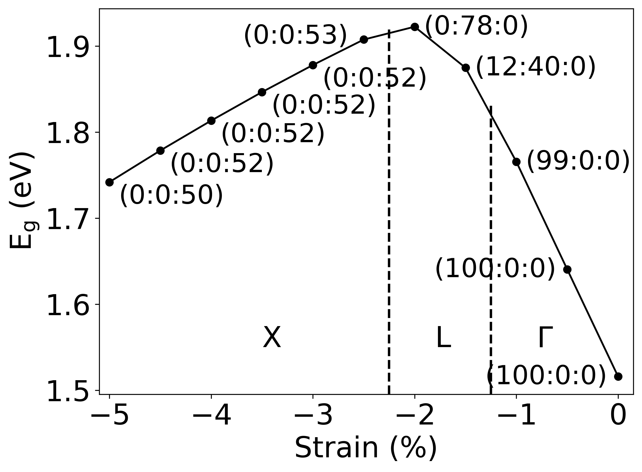
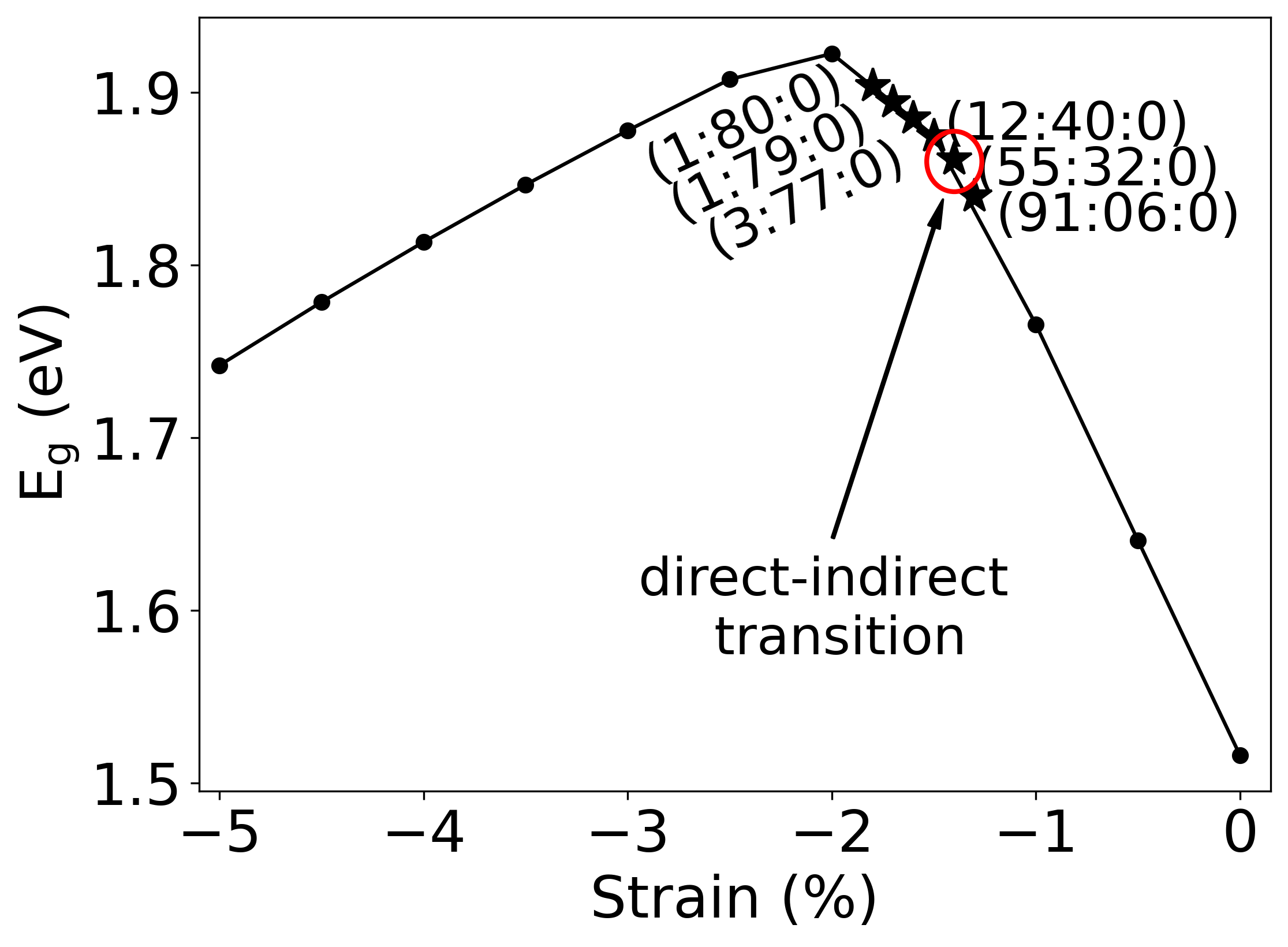
FIG. 1. Variation of the bandgap under isotropic compressive strain for GaAs0.963P0.037. The Γ-, L-, and X-BSW of the folded supercell conduction band are given in parentheses in the format (Γ:L:X). The vertical lines in (a) separate regions where the CBM changes character. In (b), the strain reso- lution is increased to determine the point of direct-indirect transition more accurately, indicated by the red circle (where the highest BSW changes from Γ to L).

band minima (CBM) change their position in reciprocal space under strain. We have also shown that the CBM occurs only at the Γ-, L-, and (near) X-point in the band structure under strain. Therefore, it is sufficient to trace the conduction band (CB) at these points to determine the nature of the bandgap. As in our previous study on binary systems, we focus here on analyzing ternary III-V compounds with zincblende structures. For these struc- tures in the 6 × 6 × 6 supercell dimensions chosen here, the Γ-, L- and X-point of the primitive band structure

Fold To The Γ-Point In The Supercell . Therefore,

it is sufficient to calculate the BSWs of solely the CB at the Γ-point in the supercell calculation to determine the

4

nature of the bandgap. Consequently, we performed the supercell calculations by sampling the reciprocal space only at the Γ-point and unfolded the CB.

Figure 1 shows the steps for determining the bandgap nature from supercell calculations more clearly. Figure 1a shows the bandgap variation for GaAsP with 3.7% P con- centration under isotropic compressive strain. The Γ-, L-, and X-BSWs of the folded supercell CB are given in parentheses. This shows 100% Γ-BSW for the unstrained structure in line with the direct bandgap. With increas- ing strain, the Γ-BSW decreases (first number in brack- ets), and the L-BSW increases (second number in brack- ets). After a certain amount of strain, the L-character of the CB dominates. The bandgap becomes indirect in nature. Notably, once the strain values reach the point of direct-indirect transition (DIT) in the bandgap nature (around –1.5% strain), the bandgap values begin to de- crease further with additional strain. This trend is like what we previously observed in binary III-V semicon- ductor systems, where a strong dependence of the band energies (E) on the wavevectors (k) under strain was found, leading to a non-monotonic variation of bandgap

Values With Strain . Moreover, We Found That Such

non-monotonic behaviour in bandgap values under strain points to a DIT .

In Ternary Iii-V Semiconductor

systems, we have now found that similar non-monotonic behaviour in bandgap values under strain also indicates a DIT. Further compressing the system then leads to a transition of the CB character from L to X.

In Fig. 1b, we show calculations with increased res- olution in strain to accurately determine the transi- tion to L corresponding to the sought point of DIT at −1.4% strain. We define the last strained structure with bandgap of direct nature before the transition to the in- direct bandgap as the transition point (the red circle in Fig. 1b). In the Supplemental Material (Fig. S1 ), we have given the EBSs of GaAs0.963P0.037 for different strain values. These confirm our analyses.

If the difference in BSW between different points in k-space is large, the nature of the bandgap can be unan- imously determined.

However, Close To The Transition

points, in some cases, the differences are more subtle (Fig. S2 ). We, therefore, set a cut-off criterion of 20% BSW. If the Γ-BSW is larger than the cut-off cri- terion, then the direct transition has a finite probability even if the L- or X-BSW is larger than the Γ-BSW. In such cases, the bandgap is called “partially direct”. This defines a “region of uncertainty” in the bandgap nature.

We chose the 20% cut-off criterion because this produces results that agree best when compared to the experiments for several systems. For the GaPBi system, however, the 10% BSW cut-off criterion produces the best agreement.

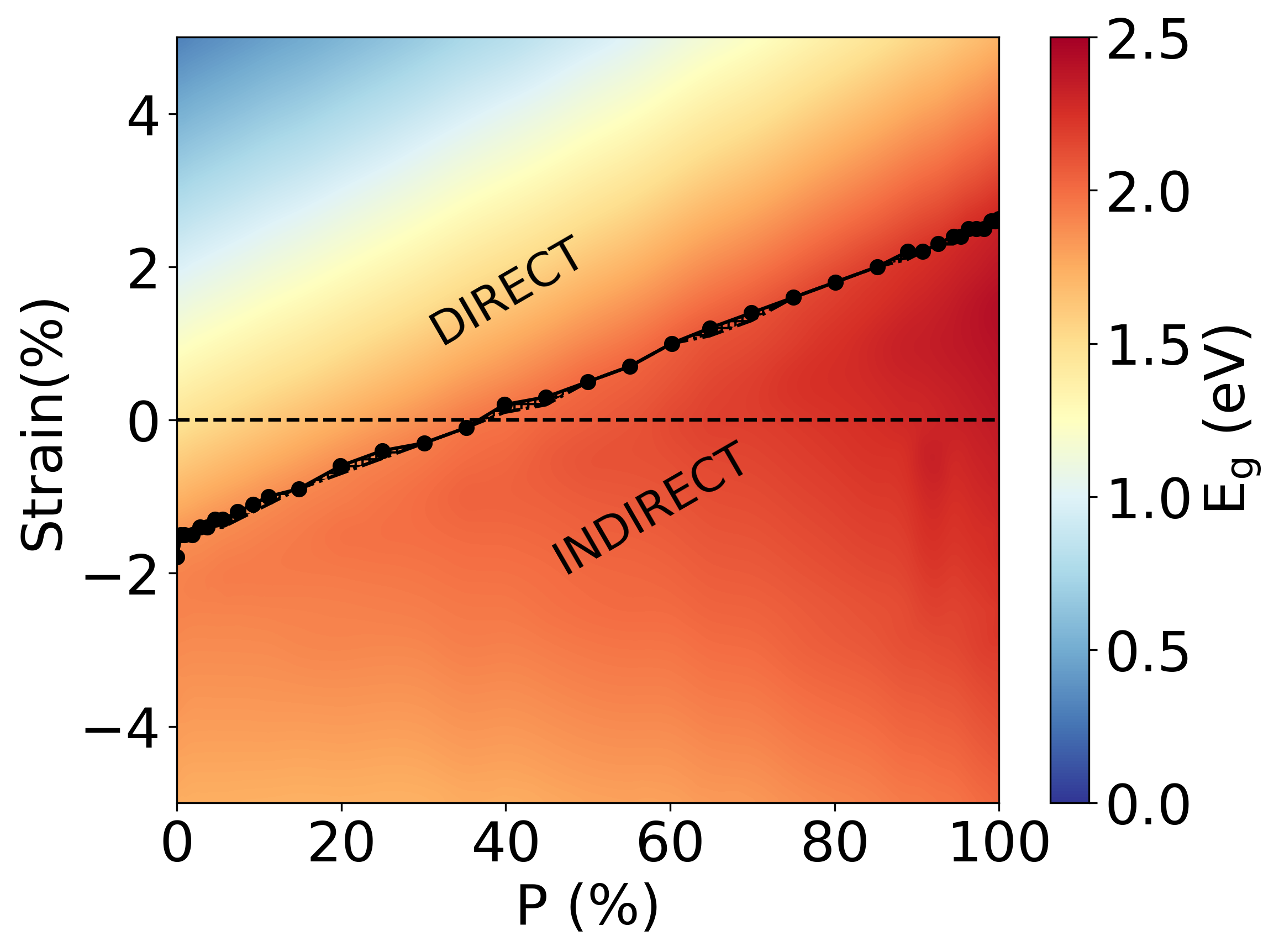
In some systems such as GaAsN, the band originating from the added nitrogen atoms, the so-called “defect N state” [54, 106–109], is strongly dispersed under strain (Figs. S3b and S4b ). Therefore, we set another cut- off criterion of 20% BSW as a minimum limit for a (de- fect) eigenstate to be considered an eigenstate (Fig. S5 FIG. 2. Isotropic strain for GaAsP. The variation of bandgap magnitudes (Eg) and type as a function of composition and strain. The dashed black horizontal line indicates unstrained GaAsP. The black circles are the calculated DIT points. The direct and indirect enclosed regions describe the nature of bandgap being direct and indirect, respectively. The hatched pattern region is the “uncertainty region” (see Sec. III).

). Starting from the lowest unoccupied CB, we search for eigenstates until the cut-off BSW criterion is met, at which point we consider it to be the redefined CB. If none of the CBs satisfy the cut-off criterion, we use the lowest CB for determining the bandgap nature. Accordingly, in these cases, we calculate the bandgap values as the en- ergy difference between the highest VB and the redefined CB. When redefining, unoccupied CB states that do not satisfy the cut-off criteria are disregarded. This led to an increase in the bandgap values, as is observed in Fig. S5 .

Results

In this section, we present the bandgaps calculated for different materials and determine their nature accord- ing to the above protocol.

We Mapped The Bandgaps

in terms of their size and nature for various strained ternary III-V compounds.

We Start With Two Impor-

tant ternary III-V semiconductor materials, GaAsP and GaAsN. Then we show selected data for the material sys- tems GaPSb, GaAsSb, GaPBi, and GaAsBi.

Gaasp

For the case of isotropic strain, Fig. 2 shows the bandgap as a function of composition (x = 0–100% in GaAs1−xPx) from 5% tensile to 5% compressive strain.

The bandgap value varies between 0.32–2.42 eV in the strain regime investigated. For the same amount of P

5

concentration, the bandgap primarily increases in mov- ing from tensile to compressive. Furthermore, the figure shows that in going from compressive to tensile strain, the DIT occurs at a higher concentration of P atoms.

The dashed horizontal line marks the data correspond- ing to the unstrained structures for different fractions of P. The intersection of this line with the DIT line shows at which percentage of phosphorous contribution the un- strained structure shows a DIT. This transition occurs at x = 37%. Here, the bandgap shows a value of 1.96 eV.

The terms direct and indirect in the figure correspond to the area where the bandgap is direct and indirect, respec- tively. Due to the similarity with commonly used phase diagrams, we call this representation a “bandgap phase diagram”. This and the following figures thus provide a 2D representation of the bandgap phase diagram for the ternary materials.

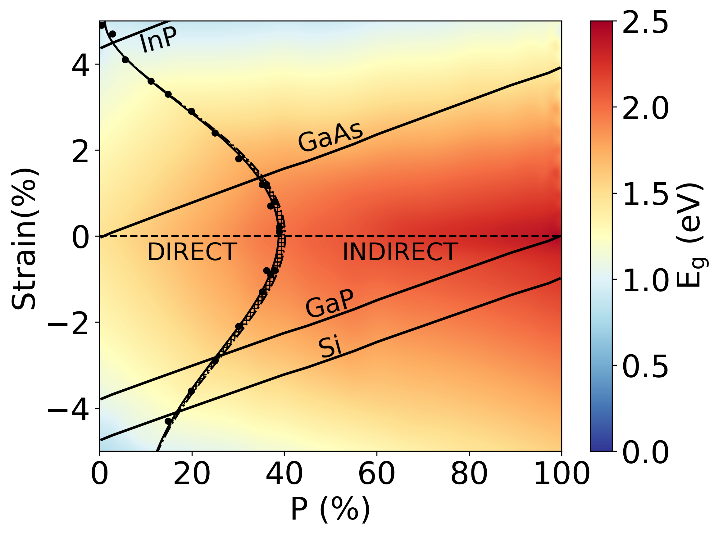
For the biaxial strain regime, Fig. 3 shows the bandgap phase diagram for GaAsP as a function of composition from 5% tensile to 5% compressive strain. The value of the bandgap varies in a range of 0.82–2.42 eV. For the same amount of P atoms, the bandgap reaches a max- imum around the unstrained structure and gets smaller for tensile as well as compressive strain. This is different from the isotropic strain case. For unstrained GaP, the bandgap value is 2.36 eV. The nature of the bandgap also shows a different trend compared to Fig. 2. The range of strain around the unstrained structure where a direct bandgap is found gets smaller for higher amounts of P.

This is in line with GaAs (0% P) being a direct and GaP (100% P) being an indirect semiconductor. The largest amount of P concentration where a direct semiconductor is found is 39–40% P in the unstrained structure. This is similar to the previous experimental result (45% P) [10, 110].

One of the most common approaches to experimentally realize biaxial strain in III-V semiconductors is epitaxial growth. As pointed out in Ref. , biaxial strain can be used to model epitaxial growth. We thus investigate the effect of different substrates in our bandgap phase dia- gram (Fig. 3), where each solid line corresponds to one substrate: GaAs, GaP, InP, or Si. These solid lines indi- cate how much biaxial strain would develop in the GaAsP system as the respective value of % P when grown on the respective substrates under idealized conditions. The (substrate) strains are calculated according to Eq. (2):

(2)

where asub is the equilibrium lattice parameters of the substrates, and a is the lattice parameters of unstrained GaAsP systems at their respective P concentrations.

E.g., for 100% P, the strain on the GaP substrate is zero, while growing GaAs (0% P) on GaP would result in 3.8% in-plane compressive strain. This, of course, neglects de- fect formation and strain relaxations and assumes per- fect epitaxial growth. Clearly, by choosing different sub- strates, the nature can be changed, and the size of the FIG. 3. Biaxial strain for GaAsP. The variation of bandgap magnitudes (Eg) and type as a function of composition and strain. The dashed black horizontal line indicates unstrained GaAsP. The black circles are the calculated DIT points. The DIT points are fitted with a 5th-order polynomial. The direct and indirect enclosed regions describe the nature of bandgap being direct and indirect, respectively. The hatched pattern region is the “uncertainty region” (see Sec. III). Solid black lines indicate the substrate lines under “epitaxial growth” model.

bandgap can be tuned over a wide range. We refer to the next section for a comparison of our calculations to experimental data.

Gaasn

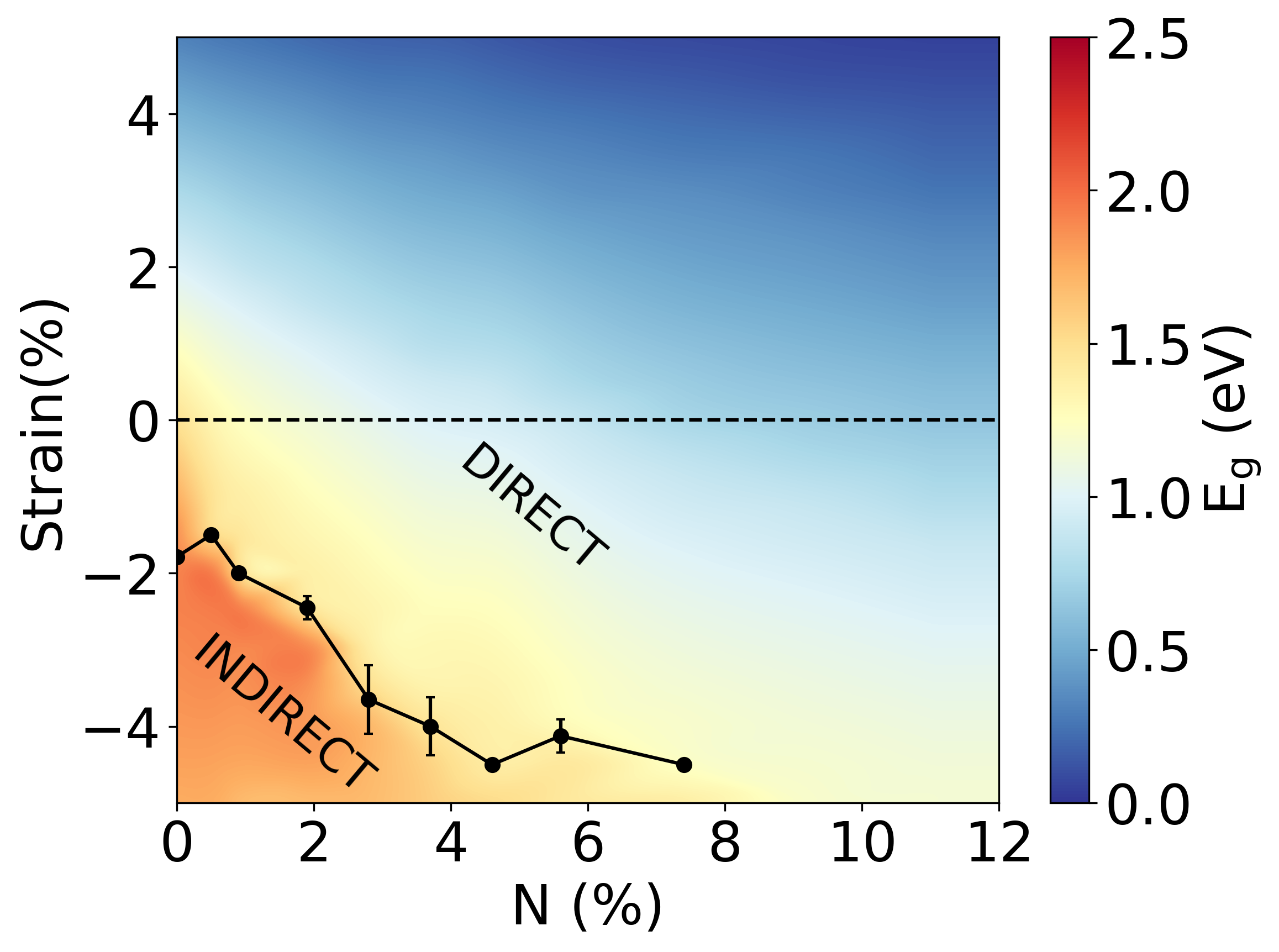
As the next material, we investigate GaAsN. First, we show results for isotropic strain, which results in the bandgap phase diagram shown in Fig. 4. The results are markedly different from GaAsP, and the data set is much more limited. In this case, we found a strong dependency of the bandgap on the N atoms distribution in the super- cell . We thus used 10 SQS cells for each data point in the figure and averaged the resulting bandgaps. This results in an error bar for the DIT points, which is rather large for medium amounts of nitrogen atoms due to the formation of small clusters and chains. Calculations were only possible for up to 12% N. For higher concentration and/or high compressive strain, our chosen supercell is not large enough to avoid the unphysical electronic in- teraction of N atoms with their images in the periodic boundary condition approach.

This Effect Has Already

been discussed in Ref. . For the strain and composi- tion regions where computation was possible, an indirect gap is only found for low values of % N and rather large compressive strain values. The EBSs for selected % N and strain values are shown in Figs. S3 and S4 .

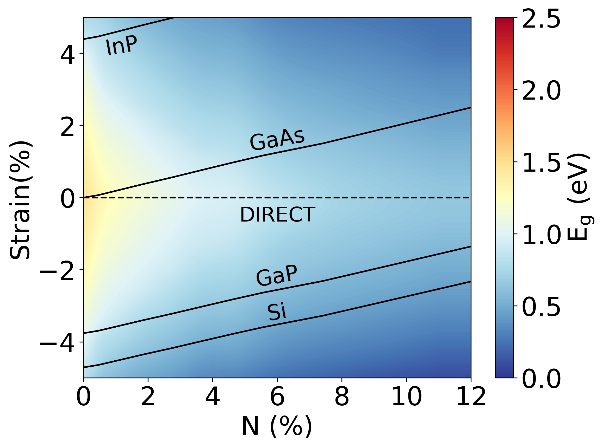
For biaxial strain in GaAsN, the data are shown in Fig. 5. In contrast to GaAsP, the bandgap gets smaller

6

FIG. 4. Isotropic strain for GaAsN (up to 12% N). The vari- ation of bandgap magnitudes (Eg) and type as a function of composition and strain. The dashed black horizontal line indi- cates unstrained GaAsN. The black circles are the calculated DIT points. Beyond 7% N, the DIT is outside the investigated strain regime. 10 SQS cells are used for each configuration and strain point. The bandgaps plotted are the average bandgaps.

The error bars indicate the standard deviation in DIT points estimation. The direct and indirect enclosed regions describe the nature of bandgap being direct and indirect, respectively.

with the increasing amount of nitrogen in the system, from 1.47 eV for the unstrained case of GaAs to 0.10 eV for the highly strained systems with a large number of N atoms.

All bandgaps computed are direct.

Epitax-

ial growth on GaAs is reasonably possible for moderate strain values and results in a variation of bandgap from 1.47 eV to 0.45 eV. For GaP and Si substrates, a large strain would be exerted on the system, and mostly lower bandgap values are found.

Gapsb, Gaassb, Gapbi, Gaasbi

The approach outlined here can be extended to other combinations of elements in III-V semiconductor mate- rials. Exemplarily, we present the bandgap phase dia- grams for four other important ternary compounds in Fig. 6. Since epitaxial growth is the most interesting ex- perimental realization method for these compounds, we only present the data for biaxial strain.

For All Compounds Investigated, We Find A Bandgap

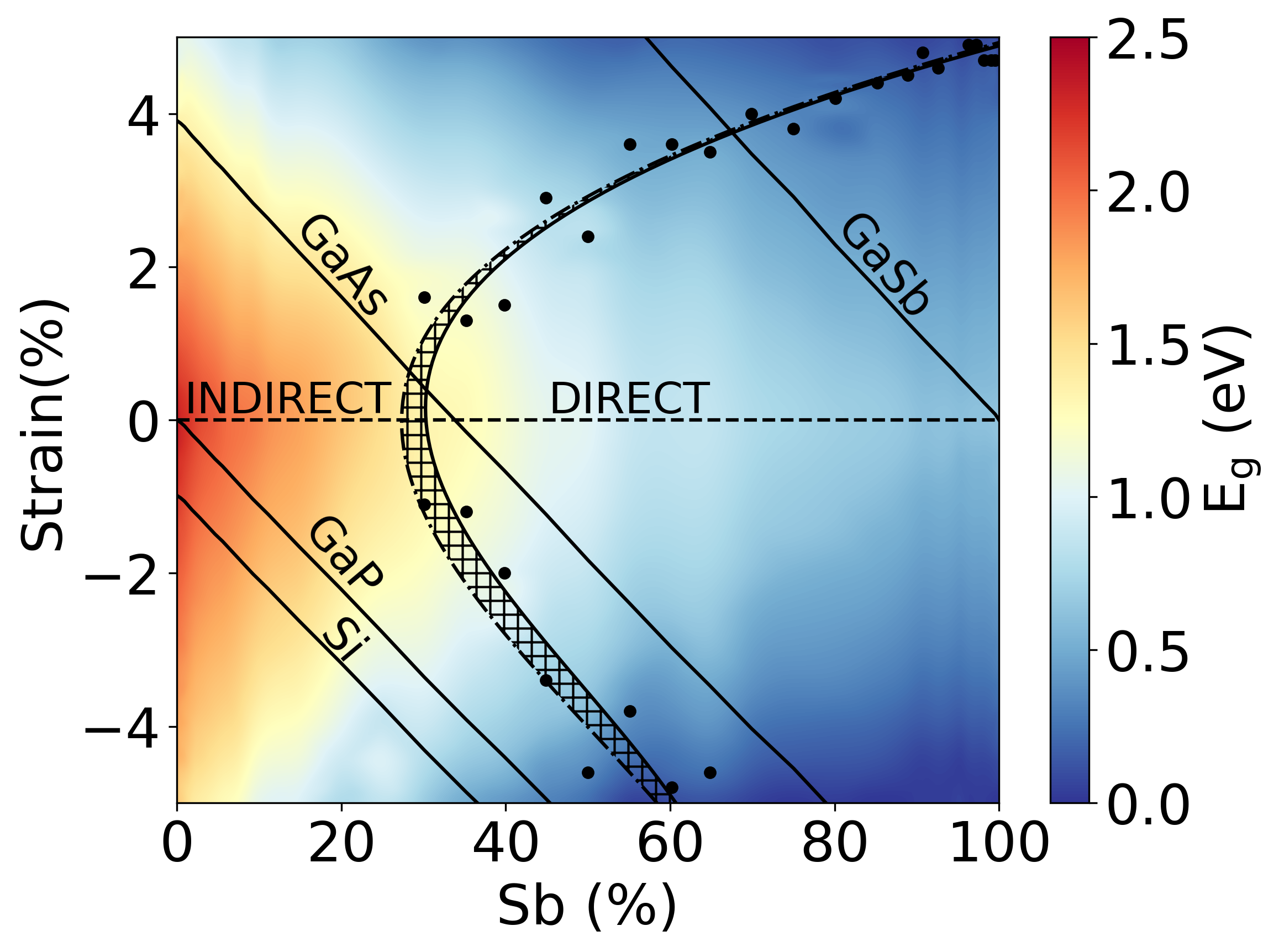
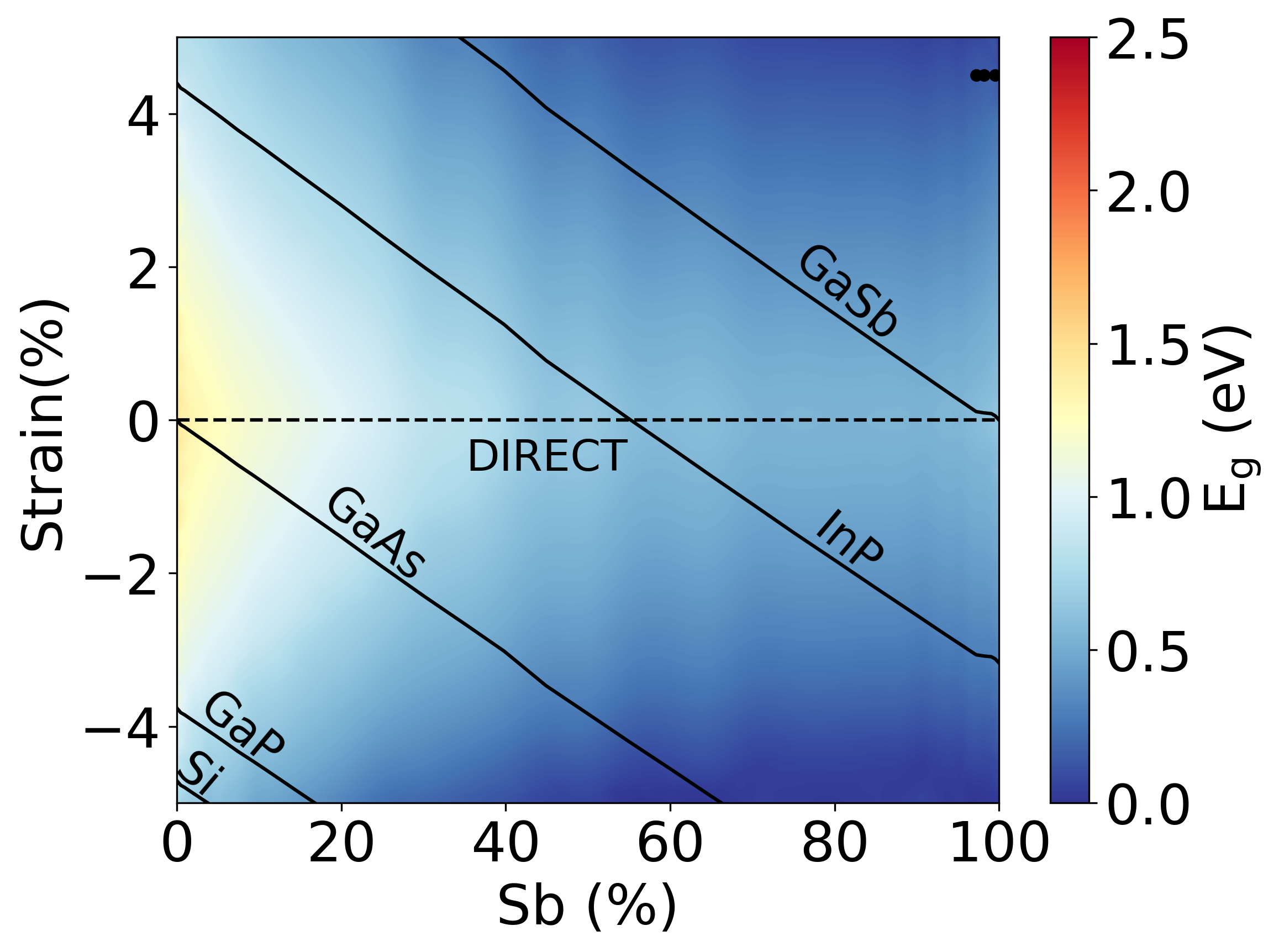
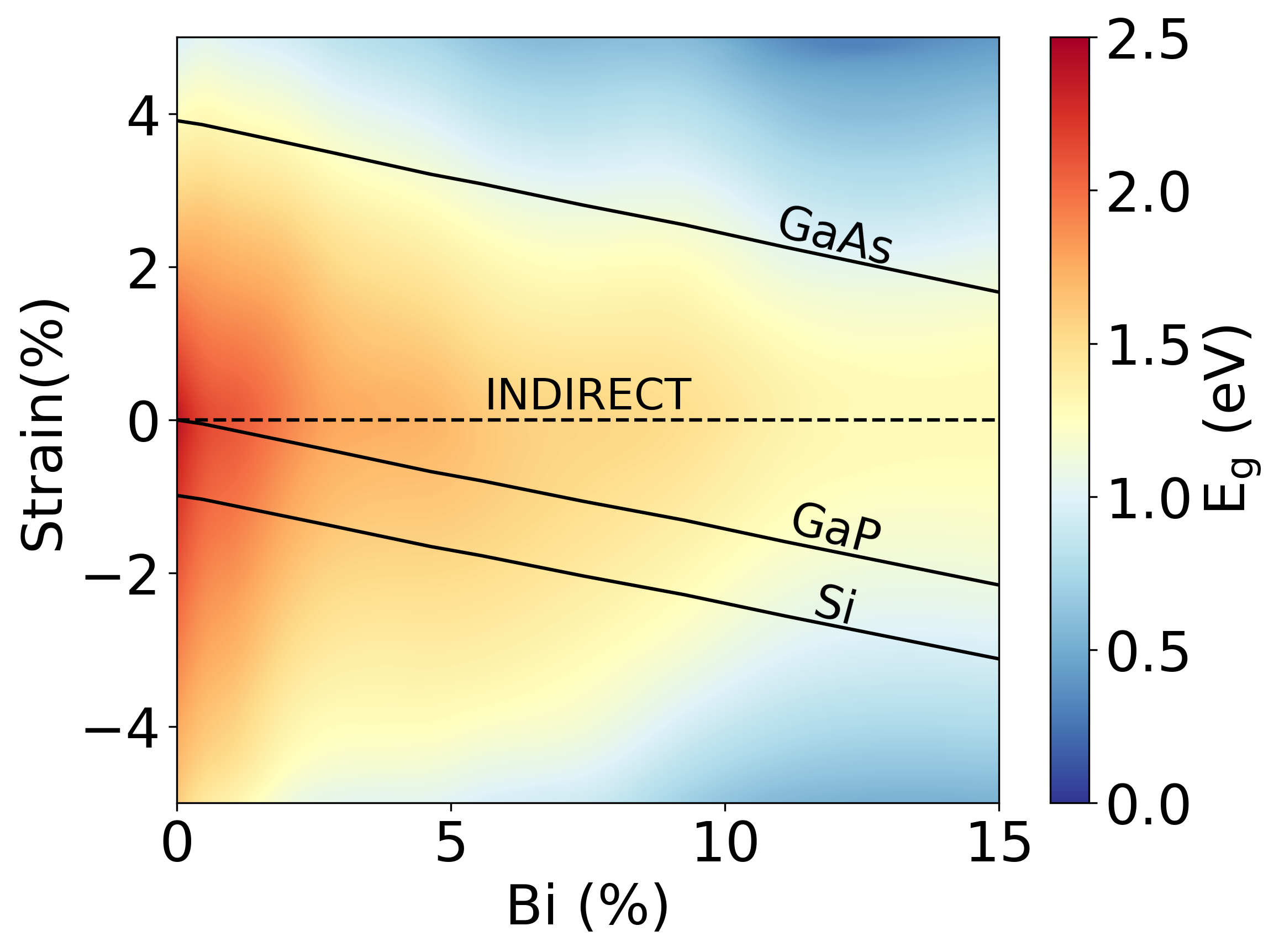
range of 0.00–2.36 eV, with the largest values found for the host materials GaP and GaAs in the unstrained case. The alloys with Sb could be investigated over the full

Range Of 0–100% Sb In Gapsb And Gaassb (Figs. 6A

and 6b). We find a DIT for unstrained GaPSb at 30% Sb concentration (Fig. 6a). For this compound, the DIT is shown as a region, including the uncertainty in deter- mining the nature of the bandgap, as outlined in Sec. III.

With the increase in the Sb fraction, the strain at which FIG. 5. Biaxial strain for GaAsN (up to 12% N). The vari- ation of bandgap magnitudes (Eg) and type as a function of composition and strain. The dashed black horizontal line indicates unstrained GaAsN. 10 SQS cells are used for each configuration and strain point. The bandgaps plotted are the average bandgaps.

All the bandgaps are direct in nature. Solid black lines indicate the substrate lines under the “epi- taxial growth” model.

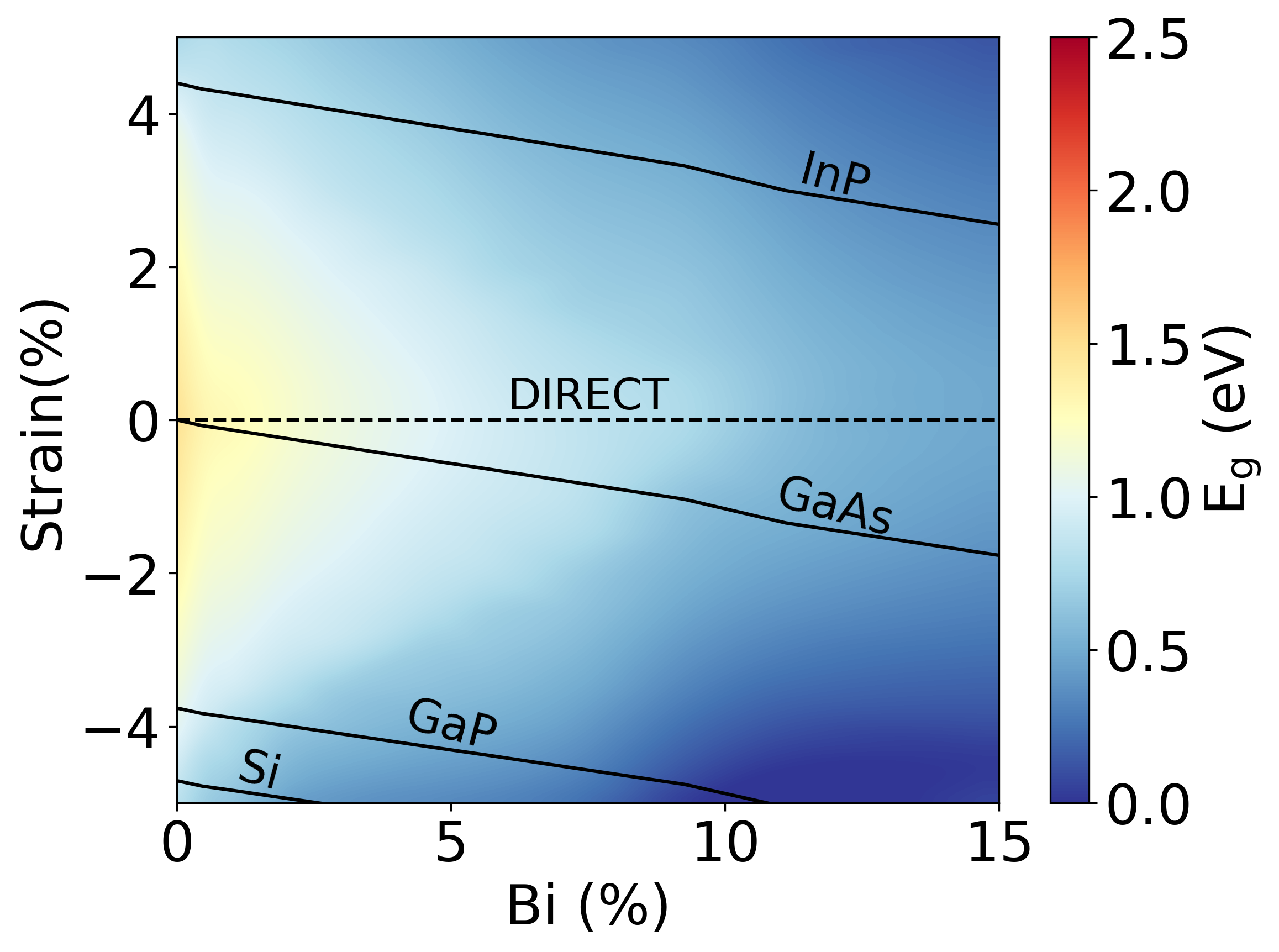
the DITs take place increases. For GaAsSb and GaAsBi, the bandgap is direct throughout the range investigated (Figs. 6b and 6d), while it is indirect for GaPBi (Fig. 6c).

Notably, we only investigate the bismides up to a frac- tion of 15% Bi. The reason is that, similar to GaAsN (Fig. S4 ), for structures with large Bi content, the strongly dispersed bands decrease the reliability in the determination of bandgap nature. Additionally, GaPBi and GaAsBi become metallic for higher Bi fractions. Al- though we find no transition within 15% Bi, it can not be excluded that the DIT appears at higher percentages of bismuth.

Again, we indicate the strain values associated with different typical substrates for epitaxial growth by solid black lines in the figures. The data show that deviat- ing from the substrate-layer lattice-matching condition quickly leads to high strain, and defects are highly likely to occur during growth. Also, Si can be used as a sub- strate for GaPSb and GaPBi epitaxial growth if the Sb or Bi content is not too large. The epitaxial growth of the respective GaAs-based materials (GaAsP, GaAsN, GaAsSb, GaAsBi) will give rise to high strain on Si- substrate throughout the whole composition region. A noticeable change in the slope in substrate lines is found close to 10% Bi and 40% Sb concentration in GaAsBi and GaAsSb, respectively. Although we did not find any structural phase transition in those regions, the origin of the change in the slope is not clear to us yet.

From The Above Discussions, It Becomes Clear That

bandgap phase diagrams can be a valuable aid in de- ciding which substrates are good choices for targeting a specific bandgap size and nature for a given ternary mate-

(D) Gaasbi

FIG. 6. Bandgap phase diagram for ternary III-V semiconductors GaEY (E= P, As; Y = Sb, Bi) under biaxial strain. The bandgap magnitudes (Eg) are shown in the color bar. The dashed black horizontal line indicates unstrained structures. The black circles are the calculated DIT points. The direct and indirect enclosed regions describe the nature of bandgap being direct and indirect, respectively. The hatched pattern region is the “uncertainty region” (see Sec. III). Solid black lines indicate the substrate lines under the “epitaxial growth” model.

rial. And vice versa, which material to grow for a specific application and a given substrate? We will discuss this further in the next section.

All Data Were Derived From Dft Computations To

this point. In Table I, we now compare our calculated bandgaps with experimental data from measurements on heteroepitaxial layer structures. The GaAsP/GaAs sam- ples were grown by low-pressure hydride vapor phase epitaxy (LP-HVPE). Further details can be found in

Ref. . The Remaining Samples Were Grown By Met-

alorganic vapor phase epitaxy (MOVPE). The details of the growth characteristics of the MOVPE samples can be found in Refs. [22, 72, 112–117].

Experimentally,

the layer thickness and bandgaps of the MOVPE sam- ples were determined using X-ray diffraction and room- temperature photoluminescence (RT-PL), respectively.

Except for GaPSb samples from Ref. , in which cases, the PL were measured at 10 K. The comparison of the experimental bandgaps with our computed results shows good agreement. The deviation is determined with respect to the root-mean-square devi- ation (RMSD) from all available experimental samples.

For most structures, the RMSD is around 0.1 eV. Most computed values deviate by less than 10% from the ex- perimental values (exceptions are discussed separately); in the case of GaAsP, the deviation is even more ac-

8

TABLE I. Comparison of the calculated bandgaps for investigated ternary III-V semiconductors under biaxial strain with experiments. The experimental data are for the heteroepitaxial layer structures, and the bandgaps are determined from photoluminescence (PL) measurements. The “I” in the brackets indicate the indirect nature of the bandgap. The remaining

No Rt-Pl Observed

a For GaPSb samples, no specific thicknesses were reported in the reference. curate (<1%).

This Confirms Our Previous Findings On

unstrained structures that the DFT protocol we devel- oped gives excellent agreement to experimental bandgaps [11, 40, 44, 45]. In this study, we show that it is also ap- plicable to compound semiconductors under strain. For samples with very small layer thickness, the matching of experiment and computation is less good. This can be ob- served for GaAsSb/GaAs thin samples with RMSD of ca.

0.4 eV. We attribute this to the 2D quantum confinement effect, which is found for thin samples. This confinement effect leads to an increase in the bandgap with respect to thicker samples . This effect is not captured in our computational model as the calculations were performed for 3D periodic strained structures. The large deviation

Observed For Gaasn/Gap And Gaasn/Si Samples Can

not be explained by this effect alone, though. An addi- tional effect here is the strong dependency of the bandgap on the distribution of N atoms which has been found for

Unstrained Gaasn Before . The Dependency Is Fur-

ther amplified under large strain (around 3%, see Fig. 5) in those samples. In the case of GaAsN/GaAs samples, where the N concentration investigated was around 1– 5%, the strain is relatively small (<1%), resulting in bet- ter agreement with the experiment as compared to the GaAsN/GaP and GaAsN/Si samples.

Observed For Gapsb/Si And Gapbi/Gap Samples. This

is consistent with our findings that those materials show indirect bandgaps (Figs. 6a and 6c). Experimental mea-

(D)

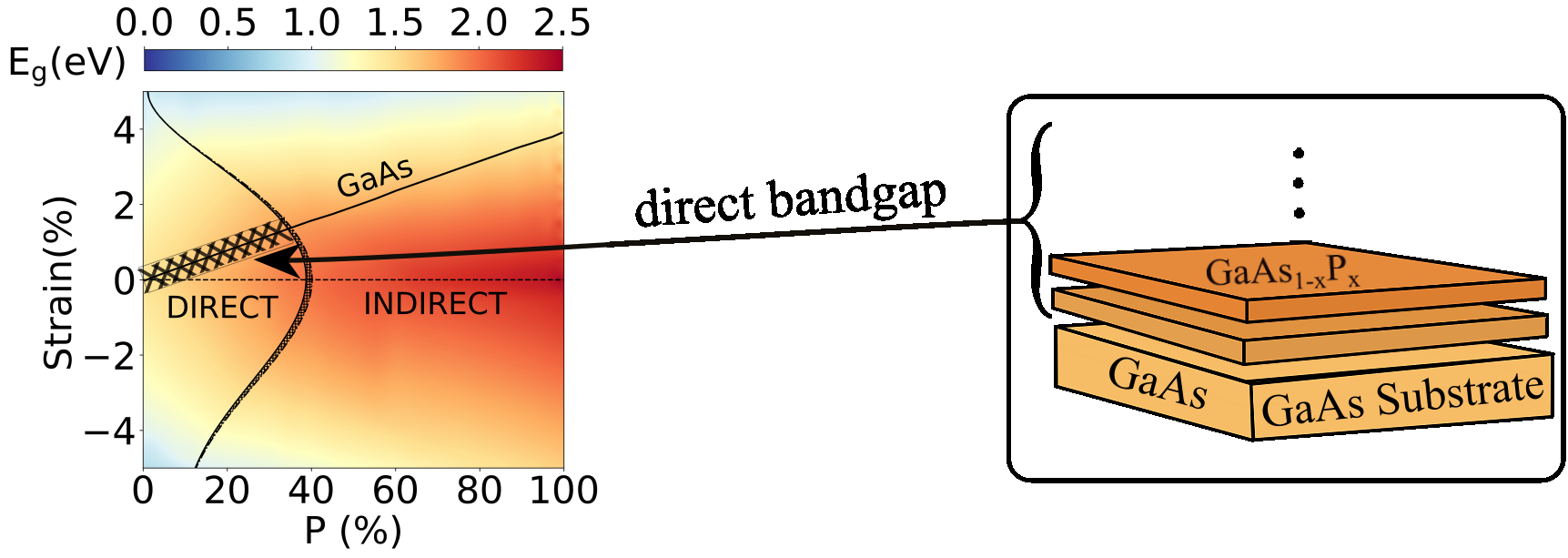
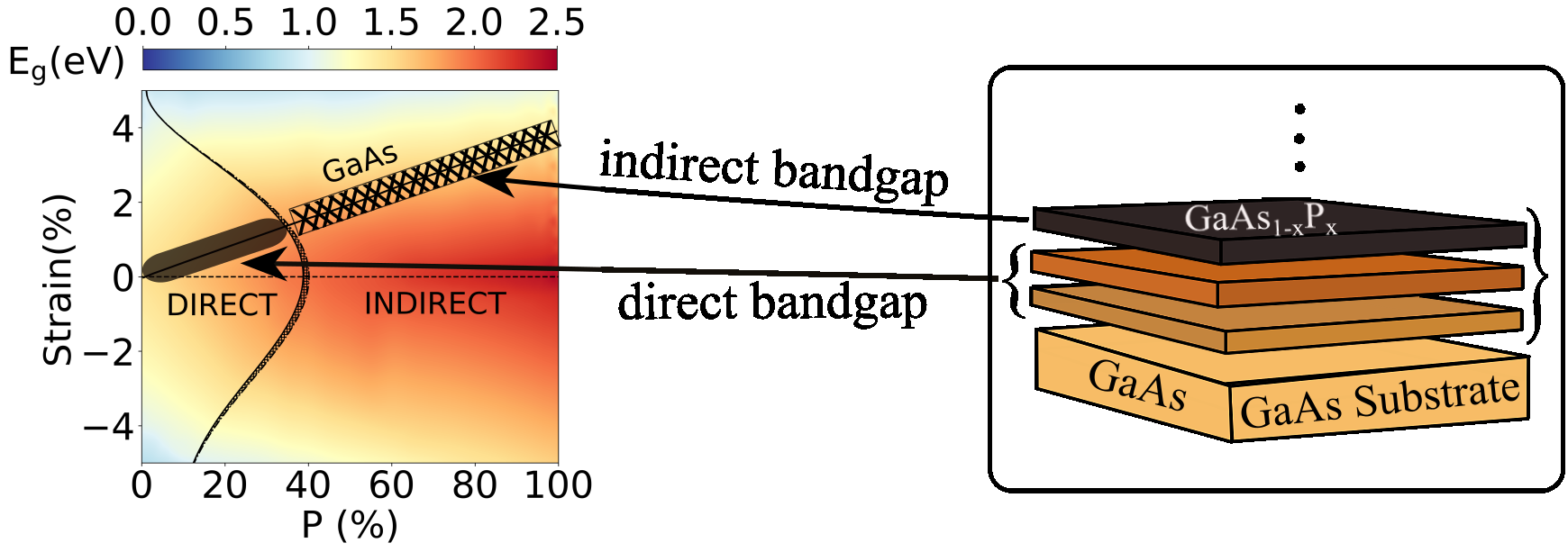
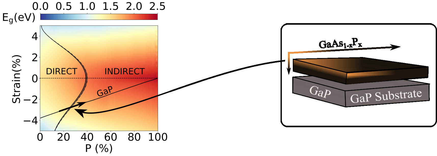
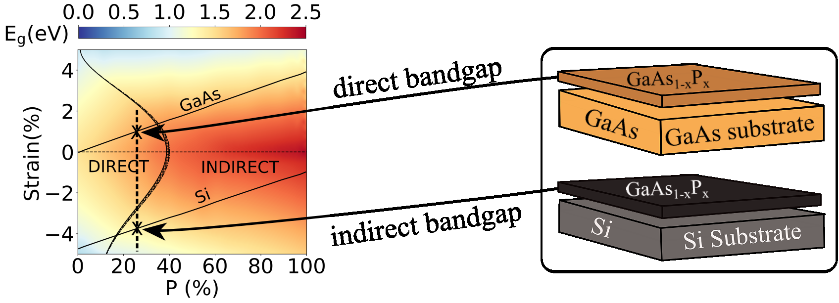
FIG. 7. Proposals on how the bandgap phase diagram of biaxially strained GaAsP can be used in designing optoelectronic devices. (a) Defines the bound of composition region for creating a QWH with direct bandgap GaAsP on GaAs substrate. (b) Choosing the different composition regions appropriately to make a multijunction photovoltaic with successive direct and indirect cells on the GaAs substrate. (c) In the vicinity of the transition point, the bandgap properties of the GaAsP epilayer on the GaP substrate can be changed by appropriately varying the composition. (d) Depending on the choice of substrate, GaAs or Si, the particular composition indicated by the vertical line can be made direct or indirect bandgap, respectively.

10

surements of the magnitude of the indirect bandgaps are not available yet. The consistent agreement between the experiment and calculated bandgaps (both in magnitude and in nature) suggests that we are able to quantitatively predict the bandgap over a wide range of compounds, compositions, and strain regions. However, as discussed above, the ef- fect of 2D confinement is also crucial for relatively thin quantum well heterostructures and, hence, needs further investigation.

Finally, based on the bandgap phase diagram, we pro- pose several design strategies to optimize the selection of material combinations for achieving specific optical ap- plications and new design principles for devices (Fig. 7).

In Fig. 7a, we propose a quantum-well heterostructure (QWH) composed of biaxially strained GaAsP on GaAs substrate. As the QW layers are made out of a single ma- terial with varied composition only, the epitaxial growth could be performed efficiently. The bandgap phase dia- gram shows the areas in compositional phase space where a direct bandgap in GaAs1−xPx can be achieved (x < 34%). For x > 35%, the bandgaps are indirect and hence, are inappropriate for the heterostructure.

Figure 7b shows an efficient approach for the mono- lithic integration of multiple QWH to construct multi- junction photovoltaics. In this case, the QWHs are sep- arated by thin indirect bandgap layers of the same ma- terial as QWH but only with a different composition.

This would make the integration approach efficient, as no sample transfer is required during growth. In Fig. 7c, we propose a device with a gradual change in the bandgap properties. The concept utilizes the con- tinuous transition in the nature of bandgap with alloy concentration in the vicinity of the DIT region. At the amount of P chosen here (x = 15–35%), we propose to grow the GaAsP epitaxial layer on GaP with P concen- tration continuously changing from the direct to indirect bandgap region or vice versa. This way, changes in the bandgap magnitude, as well as the nature of the bandgap, are possible. Note that the concentration gradient can be implemented both in the horizontal and vertical di- rections.

Figure 7d shows another application of this concept. By appropriately choosing the substrate, we can tune the epitaxial layer (here: GaAsP) to show either a direct or indirect bandgap. Depending on the substrate, GaAs, or Si, the particular composition indicated by the vertical line will show direct or indirect bandgap, respectively.

Summary

Using density functional theory and the concept of band unfolding, we developed a first-principles compu- tational protocol for the comprehensive mapping of the bandgap magnitude and type over a wide range of compo- sition and strain values for several ternary III-V semicon- ductors. We constructed the composition-strain-bandgap relationship, the bandgap phase diagram, for several ternary III-V semiconductors: GaAsP, GaAsN, GaPSb, GaAsSb, GaPBi, and GaAsBi.

We Showed That This

way of mapping the effect of strain could be used to choose application-specific best-suited material systems and hence, is highly beneficial to device design. In addi- tion, we developed an efficient approach based on Bloch spectral density for determining the nature of bandgap from supercell calculation. Notably, our computational protocol can be generalized to explore the vast chemical space of III-V materials with all other possible combi- nations of III- and V-elements. The comparison to ex- perimental bandgap data underlines the accuracy of the computational approach chosen. This approach will be extended to more complex materials in the future.

We Thank The German Research Foundation (Dfg) In

the framework of the Research Training Group “Func- tionalization of Semiconductors” (GRK 1782) for fund-

Ing This Project And To Hrz Marburg, Goethe-Csc

Frankfurt, ZIH Dresden, and HLR Stuttgart for provid- ing the computational resources.

Repository

(https://doi.org/10.17172/NOMAD/2023.02.27-1).

Mate-

rial .

Web

browser.

//Bmondal94.Github.Io/Bandgap-Phase-Diagram/,

last accessed 10.05.2023).

Bandstructures Of Gaasp, Gaasn, And Gaasn Under

selected isotropic strain values; a visual representation of the assessment of uncertainty in the bandgap nature near the direct-indirect transition region; the DFT calcu- lated bandgap values for all the systems described in the manuscript; the details of the interpolation procedure; and the bandgap phase diagrams.

P. Y. Yu And M. Cardona, Fundamentals Of Semicon-

ductors: Physics and Materials Properties, Graduate Texts in Physics (Springer Berlin Heidelberg, 2010).

Maßmeyer,

J. Glowatzki, A. Ruiz Perez, S. Reinhard, W. Stolz, and K. Volz, Electron. Lett. 58, 70 (2022). C. Fuchs, A. Br¨uggemann, M. Weseloh, C. Berger,

C. M¨Oller, S. Reinhard, J. Hader, J. V. Moloney,

A. B¨aumner, S. W. Koch, and W. Stolz, Sci. Rep. 8, 1422 (2018).

S. Mokkapati And C. Jagadish, Mater. Today 12, 22

(2009). F. Dimroth, T. N. D. Tibbits, M. Niemeyer, F. Predan, P. Beutel, C. Karcher, E. Oliva, G. Siefer, D. Lackner, P. Fuß-Kailuweit, A. W. Bett, R. Krause, C. Drazek, E. Guiot, J. Wasselin, A. Tauzin, and T. Signamarcheix, B. Mitchell, G. Peharz, G. Siefer, M. Peters, T. Gandy, J. C. Goldschmidt, J. Benick, S. Glunz, A. Bett, and F. Dimroth, Prog. Photovolt: Res. Appl. 19, 61 (2011).

S. P. Philipps, F. Dimroth, and A. W. Bett, in McEvoy’s Handbook of Photovoltaics (Third Edition), edited by S. A. Kalogirou (Academic Press, 2018) pp. 439–472.

A. Beyer, W. Stolz, and K. Volz, Prog. Cryst. Growth Charact. Mater. 61, 46 (2015). I. Vurgaftman, J. R. Meyer, and L. Ram-Mohan, J.

Appl. Phys. 89, 5815 (2001).

P. Ludewig, L. Bannow, S. W. Koch, R. Tonner, And

K. Volz, Appl. Mater. Today 6, 22 (2017).

P. Ludewig, S. Reinhard, K. Jandieri, T. Wegele,

A. Beyer, L. Tapfer, K. Volz, and W. Stolz, J. Cryst. Growth 438, 63 (2016). S. Liebich, M. Zimprich, A. Beyer, C. Lange, D. J.

Franzbach, S. Chatterjee, N. Hossain, S. J. Sweeney, K. Volz, B. Kunert, and W. Stolz, Appl. Phys. Lett. 99, 071109 (2011).

O. Supplie, O. Romanyuk, C. Koppka, M. Steidl,

A. N¨agelein, A. Paszuk, L. Winterfeld, A. Dobrich, P. Kleinschmidt, E. Runge, and T. Hannappel, Prog. Cryst. Growth Charact. Mater. 64, 103 (2018).

G. Stringfellow, in Met. Vap. Phase Ep. (Wiley, 2019) pp. 19–69.

B. Kunert, And

W. Stolz, J. Cryst. Growth 311, 2418 (2009). M. Feifel, J. Ohlmann, J. Benick, T. Rachow, S. Janz, M. Hermle, F. Dimroth, J. Belz, A. Beyer, K. Volz, and B. Kunert, J. Koch, T. Torunski, K. Volz, and W. Growth 272, 753 (2004).

K. Volz, T. Torunski, B. Kunert, O. Rubel, S. Nau, S. Reinhard, and W. Stolz, J. Cryst. Growth 272, 739 (2004).

J. Veletas, T. Hepp, K. Volz, and S. Chatterjee, J. Appl. Phys. 126, 135705 (2019).

L. Duschek, K. Jandieri, R. Tonner, W. Stolz, And

K. Volz, J. Phys. D. Appl. 49, 075108 (2016).

By

S. Wang and P. Lu (Springer, Singapur, 2019) pp. 37– 58. P. E. Van Camp, V. Van Doren, and J. T. Devreese, Phys. Rev. B 41, 1598 (1990).

R. F. Potter, Phys. Rev. 103, 861 (1956). P. A. Alekseev, V. Sharov, B. Borodin, M. S. Dunaevskiy, R. Reznik, and G. E. Cirlin, Microma- chines 11, 581 (2020).

A. K. Katiyar, K. Y. Thai, W. S. Yun, J. Lee, and J.-h. Ahn, Sci. Adv. 6, eabb0576 (2020). B. Lim, X. Cui, and S. P. Ringer, Phys. Chem.

Phys. 23, 5407 (2021). G. Signorello, E. L¨ortscher, P. Khomyakov, S. Karg, D. Dheeraj, B. Gotsmann, H. Weman, and H. Riel, Nat.

Commun. 5, 3655 (2014). G. Signorello, S. Karg, M. T. Bj¨ork, B. Gotsmann, and H. Riel, Nano Lett. 13, 917 (2013).

L. Balaghi, G. Bussone, R. Grifone, R. H¨ubner, J. Gren- zer, M. Ghorbani-Asl, A. V. Krasheninnikov, H. Schnei- der, M. Helm, and E. Dimakis, Nat. Commun. 10, 2793 (2019).

J. Gr¨onqvist, N. Søndergaard, F. Boxberg, T. Guhr, S. ˚Aberg, and H. Q. Xu, J. Appl. Phys. 106, 053508 (2009).

L. Francaviglia,

M. D¨oblinger, S. Matich, A. FontcubertaMorral, and M. Stutzmann, Nano Lett. 16, 7098 (2016). Montazeri, M. Fickenscher, L. Smith, H. E. Jack- son, J. Yarrison-Rice, J. H. Kang, Q. Gao, H. Hoe Tan, C. Jagadish, Y. Guo, J. Zou, M. Pistol, and C.

Pryor, Nano Lett. 10, 880 (2010). N. Sk¨old, L. S. Karlsson, M. W. Larsson, M. E. Pistol, W. Seifert, J. Tr¨ag˚ardh, and L. Samuelson, Nano Lett.

5, 1943 (2005). G. Bir and G. Pikus, Symmetry and Strain-induced Ef- fects in Semiconductors, A Halsted Press book (Wiley, 1974).

Y. Sun, S. E. Thompson, and T. Nishida, J. Appl. Phys. 101, 104503 (2007). L. Tao, W. Ou, Y. Li, H. Liao, J. Zhang, F. Gan, and X. Ou, Semicond. Sci. Technol. 35, 103002 (2020).

G. Tsutsui, S. Mochizuki, N. Loubet, S. W. Bedell, and D. K. Sadana, AIP Adv. 9, 030701 (2019). H. Fang, M. Madsen, C. Carraro, K. Takei, H. S.

Kim, E. Plis, S. Y. Chen, S. Krishna, Y. L. Chueh,

12

012111 (2011). L. C. Bannow, P. Rosenow, P. Springer, E. W. Fischer, J. Hader, J. V. Moloney, R. Tonner, and S. Koch, Model. Simul. Mater. Sci. Eng. 25, 065001 (2017).

N. G. Anderson and S. D. Jones, J. Appl. Phys. 70, 4342 (1991). Y. Tan, M. Povolotskyi, T. Kubis, T. B. Boykin, and G. Klimeck, Phys. Rev. B 94, 045311 (2016).

J. M. Jancu, R. Scholz, F. Beltram, and F. Bassani, Phys. Rev. B 57, 6493 (1998). P. Rosenow, L. C. Bannow, E. W. Fischer, W. Stolz, K. Volz, S. Koch, and R. Tonner, Phys. B 97, 075201 (2018).

B. Mondal and R. Tonner-Zech, Phys. Scr. 98, 065924 (2023).

Y.-S. Kim, M. Marsman, G. Kresse, F. Tran, And

P. Blaha, Phys. Rev. B 82, 205212 (2010). F. Tran and P. Lett. 102, 226401 (2009).

H. Jiang, J. Chem. Phys. 138, 134115 (2013). G. Rehman, M. Shafiq, Saifullah, R. Ahmad, S. Jalali-

Asadabadi, M. Maqbool, I. Khan, H. Rahnamaye-

Aliabad, and I. Ahmad, J. Electron. Mater. 45, 3314 (2016). D. Koller, F. Tran, and P. Blaha, Phys. Rev. B 85, 155109 (2012).

L. W. Wang, L. Bellaiche, S. H. Wei, and A. Zunger, Phys. Rev. Lett. 80, 4725 (1998). P. V. C. Medeiros, S. S. Tsirkin, S. Stafstr¨om, and J. Bj¨ork, Phys. B 91, 041116(R) (2015).

V. Popescu and A. Zunger, Phys. Rev. Lett. 104, 236403 (2010).

O. Rubel, A. Bokhanchuk, S. J. Ahmed, And E. Ass-

mann, Phys. Rev. B 90, 115202 (2014).

V. Popescu And A. Zunger, Phys. Rev. B 85, 085201

(2012). Y. Hinuma, A. Gr¨uneis, G. Kresse, and F. Oba, Phys. Rev. B 90, 155405 (2014).

M. G. Craford, D. L. Keune, W. O. Groves, and A. H. Herzog, J. Electron. Mater. 2, 137 (1973). I. D. Henning and H. Thomas, Phys. status solidi (a) 79, 567 (1983).

vices 41, 1475 (1994).

T. Sato And M. Imai, Jpn. J. Appl. Phys. 41, 5995

(2002). J. F. Geisz and D. Friedman, Semicond. Sci. Technol. 17, 769 (2002).

J. R. Lang, J. Faucher, S. Tomasulo, K. Nay Yaung, and M. Larry Lee, Appl. Phys. Lett. 103, 092102 (2013).

K. Hayashi, T. Soga, H. Nishikawa, T. Jimbo, And

1890 (1994). T. J. Grassman, D. Chmielewski, S. D. Carnevale, 326 (2016).

M. Weyers, M. S. Michio Sato, and H. A. Hiroaki Ando, Jpn. J. Appl. Phys. 31, L853 (1992). B. Kunert, K. Volz, J. Koch, and W. Stolz, Appl.

Lett. 88, 182108 (2006). Y. Zhao, G. Chen, S. Wang, and S. F. Yoon, Thin Solid Films 450, 352 (2004).

S. Loualiche, A. Le Corre, S. Salaun, J. Caulet, B. Lam-

Bert, M. Gauneau, D. Lecrosnier, And B. Deveaud,

Appl. Phys. Lett. 59, 423 (1998). H. Shimomura, T. Anan, and S. Sugou, J. Cryst. Growth 162, 121 (1996).

K. Nakajima, T. Ujihara, S. Miyashita, and G. Sazaki, J. Cryst. Growth 209, 637 (2000). H. B. Russell, A. N. Andriotis, M. Menon, J. Jasinski, A. Martinez-Garcia, and M. Sunkara, Sci. Rep. 6, 20822 (2016).

M. J. Jou, Y. T. Cherng, H. R. Jen, and G. B. Stringfel- low, Appl. Phys. Lett. 52, 549 (1988). Cherng, R. Cohen, and G. Stringfellow, J.

Electron. Mater. 13, 799 (1984). H. R. Jen, M. J. Cherng, and G. B. Stringfellow, Appl. Phys. Lett. 48, 1603 (1998).

T. M. Christian, D. A. Beaton, A. Mascarenhas, and K. Alberi, Proc. SPIE 10174, Int. Symp. Clust. Nano- mater. 10174, 228 (2016).

T. M. Christian, D. A. Beaton, K. Alberi, B. Fluegel,

And A. Mascarenhas, Appl. Phys. Express 8, 061202

(2015). S. J. Sweeney, Z. Batool, K. Hild, S. R. Jin, and T. Hosea, in 2011 13th Int. Conf. Transparent Opt. Net- works (2011) pp. 1–4.

S. Wang, Y. Song, K. Gu, H. Zhao, X. Chen,

H. Ye, H. Zhou, C. Kang, Y. Li, C. Cao, L. Zhang,

J. Shao, Q. Gong, and Y. Zhang, in Asia Commun. Photonics Conf. 2013 (OSA, Washington, D.C., 2013) p. AF3B.5.

D. G. Cooke, F. A. Hegmann, E. C. Young, And

T. Tiedje, Appl. Phys. Lett. 89, 122103 (2006). G. Kresse and J. Hafner, Phys. Rev. B 47, 558 (1993). B 49, 14251 (1994).

G. Kresse and J. Furthm¨uller, Phys. Rev. B 54, 11169 (1996). Furthm¨uller, Comput. Mater. Sci. 6, 15 (1996).

G. Kresse and D. Joubert, Phys. Rev. B 59, 1758 (1999). P. E. Bl¨ochl, Phys. B 50, 17953 (1994). A. Zunger, S. H. Wei, L. Ferreira, and J. Bernard, Phys. Lett. 65, 353 (1990).

A. van de Walle, M. Asta, and G. Ceder, Calphad 26, 539 (2002). van de Walle, Calphad 33, 266 (2009).

A. van de Walle, P. Tiwary, M. de Jong, D. Olmsted, M. Asta, A. Dick, D. Shin, Y. Wang, L.-Q. Chen, and Z.-K. Liu, Calphad 42, 13 (2013).

J. P. Perdew, K. Burke, and M. Ernzerhof, Phys. Rev. Lett. 77, 3865 (1996). S. Grimme, J. Antony, S. Ehrlich, and H. Krieg, J.

Chem. Phys. 132, 154104 (2010). S. Grimme, S. Ehrlich, and L. Goerigk, J. Comput. 32, 1456 (2011).

H. J. Monkhorst and J. D. Pack, Phys. Rev. B 13, 5188 (1976). See Supplemental Material for the effective bandstruc-

Tures Of Gaasp, Gaasn, And Gaasn Under Selected

isotropic strain values; a visual representation of the assessment of uncertainty in the bandgap nature near the direct-indirect transition region; the DFT calcu- lated bandgap values for all the systems described in the manuscript; the details of the interpolation proce-

Dure; And The Bandgap Phase Diagrams. The Supple-

mental Material also contains Refs. [45, 52, 95–103].

Deployment In Out-Of-Position Situations

D. Bendjaballah1, A. Bouchoucha1, M. L. Sahli1,2* and J-C. Gelin2

Abstract

Side-impact collisions represent the second greatest cause of fatality in motor vehicle accidents. Side-impact airbags have been installed in recent model year vehicle due to its effectiveness in reducing passengers’ injuries and fatality rates. In meeting these requirements, simulations of folding and deploying airbags are very useful and are widely used. The paper presents a simulation method for the deploying airbags using three materials in different working conditions. Finite element analysis is primarily used to evaluate this concept. In these simulations, the gas flow is described by the conservation laws of mass, momentum, and energy. The numerical results indicate that the FE method in this paper is capable of capturing airbag deploying process accurately.

Keywords: Airbag simulations, Out-of-position, Crash, Modeling, Out-of-position

Background

The passive safety of cars has become a very high prior- ity issue for the automotive industry. Today, there are not only one or two airbags in a car; certain models have ten times more than that. With the increasing usage of airbags, the number of accidents where the airbag itself can cause an injury to the occupant also increases

(Augenstein Et Al. 2003; Gabauer And Gabler 2010;

Audrey et al. 2011). As is well known, safety belts are also now devices designed to provide protection to the users of vehicles during crash events, minimizing the loads necessary to adapt their movement to the move- ment of the car (Freesmeier and Butler 1999; Schmitt et al. 1997). In general, the seat belt is designed to restrain the occupant in the vehicle and prevent the

Occupant From Having Harsh Contacts With Interior

surfaces of the vehicles. The airbag acts to cushion any impact with vehicle structure and has positive internal pressure, which can exert distributed restraining forces over the head and face. As a safety component of auto- mobile, an airbag decreases occupants’ injury likelihood effectively in case of an accident (Ruff et al. 2007). These safety elements can reduce the death rates on the roads, and its protection effects have been widely approved (Crandall et al. 2001; Teru and Ishikawa 2003). With computational tools such as finite element methods designed for dynamic contact problems, crashworthiness simulations can now be used with reliable accuracy to evaluate occupant protection in various collision condi- tions with safety metric/parameters such as acceleration, head injury criteria, intrusion distance, intrusion vel- ocity, and neck forces (neck injury risk or whiplash).

Thus, new types of airbag products are being developed to handle different collision scenarios.

Become Standard Equipment On Most New Passenger

vehicles (Braver and Kyrychenko 2004; Teng et al. 2007; Yoganandan et al. 2007). The airbag cushion is com- posed of a woven fabric which is rapidly inflated during a car crash. The airbag dissipates the passenger’s kinetic energy thereby reducing injury through biaxial stretching of the fabric bag and escaping gas through vents. There- fore, the performance of the airbag is greatly influenced by the mechanical properties of the fabric. Generally, air bags are designed to deploy in a crash that is equivalent to a vehicle crashing into a solid wall at 8 to 14 mph.

Air bags most often deploy when a vehicle collides with another vehicle or with a solid object like a tree. There are various types of airbags: frontal, side-impact, and curtain airbags. In general, the passenger side airbags are usually larger than the driver airbags (see Fig. 1).

Besançon, France

© The Author(s). 2017 Open Access This article is distributed under the terms of the Creative Commons Attribution 4.0 International License (http://creativecommons.org/licenses/by/4.0/), which permits unrestricted use, distribution, and reproduction in any medium, provided you give appropriate credit to the original author(s) and the source, provide a link to the Creative Commons license, and indicate if changes were made.

Bendjaballah et al. International Journal of Mechanical

Doi 10.1186/S40712-016-0070-2

Extensive studies have shown that the airbag deploy- ment in load cases consists of two occupant loading phases: a punch-out effect where the airbag bursts out of its container with the airbag and airbag module cover accelerating towards the occupant and a second loading phase during which the airbag is taking on its deployed shape and volume (membrane-loading effect). Bankdak et al. (2002) developed an experimental airbag test system to study airbag-occupant interactions during close proximity deployment. The results provided insight for simulating the effect of inflation energy and mass flow on target response. Bedard et al. (2002) found that while left-side (driver-side) impacts accounted for only 13.5% of all crashes, the fatality rate among these

Crashes Was 68.3% In Comparison To Front Impact

(48.3%), right-side impact (31.3%), and rear impact (38.4%). These studies underscore the importance of oc- cupant safety during side-impact collisions. In the last years, the current market requested to reduce the time and cost airbag development. In order to achieve this result, virtual simulations play an important role since they allow to minimize the number of experimental tests (Pei et al. 2013; Cao et al. 2014). Several simulation models of airbag were established (Wang et al. 2007). It is feasible to optimize the parameters of airbag deploy- ment using simulation technology. Experimental and numerical studies have quantified injury risks to close- proximity occupants from deploying side airbags. These studies have focused on the prevention of the most ad- verse effects of airbag deployment (Duma et al. 2003).

Other studies have proposed airbag characteristics to minimize particular biomechanical responses (Haland and Pipkorn 1996). In a more recent study, Marklund and Nilsson (2003) compared deformation patterns with experimental data as well as the computational costs associated with three different airbag deployment simu- lation methods; they concluded that the SPH method is relatively inexpensive and produces incremental deform- ation patterns that compare most closely to the experi- mental results. The process of inflation of an airbag is one of the determining factors in saving lives. The duration from the initial impact of the crash to the full inflation of an airbag is about 40 ms, and during this time, the airbag goes from being in a folded state to a fully inflated state, with a high internal pressure. After achieving this state, the airbag begins to deflate, thus providing a nice cushion for the body impacting it.

Ideally, the person in the crash should come into contact with the airbag at this time. In the present study, a large volume passenger side airbag model is developed to handle different collision scenarios. The main aim is evaluate the performance of deploying of passenger side airbag using finite element methods (FEM).

Materials

The tensile specimens were made in different airbags (P: Peugeot, R: Renault, and VW: Volkswagen) with a length of 200 mm long and a width of 40 mm. Table 1 shows the mechanical properties of the airbag.

Tensile Tests

To determine the mechanical properties of the material of airbag used in the test pieces, tensile tests were performed on Lloyd EZ20 universal testing machine in Constantine. These tests were conducted using rect- angular samples. The axial force and axial displacement acquired during a test are converted into stress and the strain in order to be used for the fabric material model.

The continuous recording of the stress-strain data was performed during both the load and unload phases. A minimum of five samples were made in order to check the repeatability of the measurements. All the data was collected by using a PC-based data acquisition system and analyzed by commercial software. The picture frame test device that is made for this study is shown in Fig. 2.

Fig. 1 a Frontal and side airbags. b Oblique view of facet occupant model in sitting posture following airbag deployment (Lim et al. 2014)

0.150

Bendjaballah et al. International Journal of Mechanical and Materials Engineering (2017) 12:12

Page 2 Of 9

Figure 3 shows the stress-strain relationship of the airbag sample under axial tensile loads. The results are showing a linear increase in extension with the increas- ing stresses. This is an expected output and it confirms with the theoretical behavior of a sample subjected to tensile stress. The rupture strain values for different airbags (R/P/VW) were 0.322, 0.441, and 0.472, respect- ively. The measured elastic parameters (i.e., Young’s modulus E and initial yield strength) and Poisson’s ratio are summarized in Table 2. The tensile tests of the woven fabrics can show differences on mechanical prop- erties because woven fabrics can resist in-plane shear loads once the yarn lock-up angle has been reached. The differences of material property on material direction can affect the shape of fully deployed bag (see Fig. 3b).

Theoretical Background

Numerical simulations of airbags use very complex and techniques such as an orthotropic model to identify the mechanical behaviors during the airbag inflation and the fluid mechanics (gas flow) to describe the inflator gas flow (pressure gradient) and improve the representation of the pressures within the airbag. To model the airbag as an orthotropic model, three material constants have to be provided. Assuming a plane stress condition, the

Ð1Þ

where σ is the normal stress and τ is the shear stress, the subscript refers to the principal material directions, i.e., the fill and warp directions. Also, ε and γ are the strain components. The material elastic constants Qij are

Ð2Þ

where E1 and E2 are the Young’s modulus in the fill and wrap directions and G12 is the shear modulus of the fabric material. νij is the Poisson ratio of the material.

The gas exerts a pressure load on the airbag causing it to expand. This expansion puts the airbag under tensile stress lowering the expansion rate. In this study, heat conduction and heat transfer is not taken into account.

Fig. 2 A photograph of Lloyd EZ20 universal testing Fig. 3 Stress versus strain using Lloyd EZ20 machine for a three different airbags at 0° and 90° and b VW airbag test specimens at

Different Angles

Table 2 Physical and mechanical properties of the airbag

Page 3 Of 9

In the deployment of an airbag, an inflator supplies high velocity gas into an airbag causing it to expand rapidly. The gas inside the airbag is assumed to be ideal, to be of constant entropy, and to satisfy the equation of state:

Ð3Þ

Here p, ρ, and e are respectively the pressure, density, and specific internal energy, and γ is the ratio of the heat capacities of the gas. The gas flow is described by the conservation laws for mass, momentum, and energy that

Ð4Þ

here, V is a volume, A is the boundary of this volume,

N Is The Normal Vector Along The Surface A, And U

denotes the velocity vector in the volume. Applying Bernoulli’s equation in the case of an ideal gas with

Ð5Þ

Here, the subscript ex denotes quantities at the throat of the tube. Furthermore u, p, and ρ denote the quan- tities inside that part of the tube that is supplying mass.

Materials And Boundary Conditions

The airbag system mainly consists of three parts: the airbag itself, the inflator unit, and the crash sensor or diagnostic unit. Thus, to study the behavior of the airbag using FE simulations, we need to have an FE model of the airbag in the folded position. A FE model of the airbag was used to simulate the test condition as shown in Fig. 5. LS-DYNA® material model FABRIC (MAT_34) is used to simulate the airbag material. It is a variation of the layered orthotropic material model. Additionally, in the LS-DYNA® material model, fabric leakage can be accounted for. However, for this CAB material, the leak- age is almost negligible and therefore no leakage is specified. The mechanical properties can be determined from the physical test. Typical material properties for airbag fabrics are taken as given in Chawla et al. (2004a) (Table 3). These properties are used to simulate inflation process of airbag (see Table 1). The car dashboard is modeled as the rectangular thin plate using a MAT_RI-

Gid Material, And The Degrees Of Freedom Are Con-

strained in all the directions. The similar properties of thermoplastic polymer are assigned for contact purposes. The porosity of the fabric is assumed zero. The nitro- gen gas is taken for inflating the airbag. Properties of nitrogen gas and initial bag conditions are shown in Table 4. The example on which we perform the study is a typical passenger side airbag. The geometric de- tails have been measured from a commercially avail- able airbag. The initial state of the airbag is a closed rectangular whose sides are to be finished to 482 × 635 mm2 and is shown in Fig. 4.

Table 3 Material properties of airbag and rigid plate used in FE

–

Table 4 Initial values used for FE simulation of the swelling of

3.33 × 10−4

Fig. 4 The initial airbag geometry in the form of a rectangular Bendjaballah et al. International Journal of Mechanical and Materials Engineering (2017) 12:12

Related Journal Articles & DOI Links

Selected peer-reviewed publications relevant to 12 Lead ECG Acquisition. Click the DOI to access the full paper (may require institutional access).

Why Choose Us?

Bangalore guidance for robotics, Spectre and autonomous systems projects.