Wind Turbine Pmsg Matlab Simulink

1

Frequency support Scheme based on parametrized power curve for

De-Loaded Wind Turbine Under Various Wind Speed

Cheng Zhong12, Yueming Lv1, Huayi Li1, JiKai Chen1, Yang Li1 1 Key Laboratory of Modern Power System Simulation and Control & Renewable Energy Technology

Corresponding Author: Cheng Zhong

Abstract: With increased wind power penetration in modern power systems, wind plants are required to provide frequency support similar to conventional plants. However, for the existing frequency regulation scheme of wind turbines, the control gains in the auxiliary frequency controller are difficult to set because of the compromise of the frequency regulation performance and the stable operation of wind turbines, especially when the wind speed remains variable. This paper proposes a novel frequency regulation scheme (FRS) for de-loaded wind turbines. Instead of an auxiliary frequency controller, frequency support is provided by modifying the parametrized power versus rotor speed (Pw-ωr) curve, including the inertia power versus rotor speed curve and the droop power versus rotor speed curve. The advantage of the proposed scheme is that it does not contain any control gains and generally adapts to different wind speeds. Further, the proposed scheme can work for the whole section of wind speed without wind speed measurement information. The compared simulation results demonstrate the scheme improves the system frequency response while ensuring the stable operation of doubly-fed induction generators (DFIGs)-based variable-speed wind turbines (VSWTs) under various wind conditions.

Furthermore, the scheme prevents rotor speed overdeceleration even when the wind speed decreases during frequency regulation control. Index Terms—DFIGs, frequency support, inertia control, power versus rotor speed curve, de-loaded control, the whole

1. Introduction

Wind power generation is the most popular renewable generation technology, and the technology of wind turbine is still improving , such as the improvement of wind turbine cooling system , fault analysis , and so on. In 2020, the new installation of wind power generation was 93 Gw, and the  total  installed  capacity  was  743  Gw  .  Approximately 95% of installed wind turbines (WTs) are Variable speed wind turbines  (VSWTs),  either  DFIGs-based  with  partially  rated converters or PMSGs-based with fully rated converters .

Unlike  conventional  power  generators,  VSWTs  have  no inherent  inertial  response  because  of  the  power  electrical converter interface. VSWTs usually do not participate in the system frequency response for operation in maximum power point tracking (MPPT) mode. Therefore, as the penetration of VSWTs increases, the inertial and frequency regulation ability of  the  whole  power  system  will  degrade,  causing  frequency stability  issues  .  Some  countries  have  required  wind plants to provide frequency support .

Many  research  studies  have  discussed  the  frequency regulation  scheme  (FRS)  for  VSWTs.  The  strategies  can  be classified into inertial response control and de-loaded control .

For inertial response control, the VSWTs still operate in MPPT mode, and the rotational kinetic energy (KE) of VSWTs is  released  to  deliver  temporary  addition  power  during frequency dips. Further, the inertial response control can divide in two subcategories : natural inertial control  and stepwise control .

For  natural  inertial  control,  the  value  of  the  addition power is determined by the frequency measurement, such as the rate of change of frequency (ROCOF) , or the frequency

Deviation  , Or Both Of Them . Considering That

the wind speed is variable and the change of the rotor speed is complicated, the auxiliary frequency controller's gains should be  selected  carefully  with  the  trade-off  considering  the frequency  regulation  performance  and  the  stable  operating range  of  the  wind  turbine.  Therefore,  some  varying  gain methods have been suggested. In , the control gains of FRS under different wind speeds is adjusted based on the wind speed.

However, the pre-determined gains are obtained by the off-line modeling analysis, and the wind speed measurement may not be obtained or inaccuracy. To improve the frequency nadir (FN) and  ensure  stable  operation  of  DFIG,  the  droop  gains  is dynamically  changes  based  on  ROCOF  in  .  In  ,  the gains of additional ROCOF and frequency deviation loops is adaptively tuned depended on the rotor speed measurement.

present  a  time  varying  gains  determined  based  on  desired frequency -response time to raise frequency nadir and eliminate frequency  second  dip.  proposed an adaptive droop gain which is a function of real-time rotor speed and wind power penetration level.

For step-wise control, the addition frequency power is determined by the pre-set power surge function, such as step function , ramp function  or torque limit function .

Compared  with  natural  inertial  response,  the  inertial  power using the step-wise control can be properly tuned according to different  shapes  in  terms  of  its  magnitude  and  duration.  An optimization approaches employing the genetic algorithm are proposed  to  maximize  the  released  energy  from  the  wind turbine during its overproduction period .However, during the  rotor    speed  recovery  period,  the  output  power  of  wind turbine reduced  and may cause a secondary frequency drop [31, 32].In  ,the  incremental  power  varies  with  the  rotor speed  and  wind  power  penetration  levels  during  the overproduction period, and then, the reference power smoothly decreases with time and rotor speed during recovery period.

For inertial response control, because of the limit of the rotor kinetic energy, it only affords for seconds-term frequency support. While, for the de-loaded control, VSWTs reserve a part of  the  active  power  through  pitch  angle  control  , over-speed control , or combination of both . It can provide a minutes-term primary frequency support.

Due  to  rotor  speed  limit,  the  over-speed  de-loaded control is only adapted for low wind range. In , three wind speed modes are defined: low wind speed mode where de-loaded operation is merely by rotor speed control; medium wind speed mode where de-loaded operation is conducted by combining pitch angle control and rotor speed control; and high wind  speed  mode  where  modified  pitch  angle  control  alone.

However, it required accuracy wind speed information to judge the wind speed mode, and the calculation of de-loaded power reference need both parameters of wind turbine and wind speed.

present  a  variable  droop  control  strategy  that  considers optional rotor kinetic energy. However, the rotor kinetic energy estimation required the wind speed information and parameters of  wind  turbine.    proposed  a  comprehensive  frequency control  that  combines  the  temporary  power  injection  control and  power  reserve  control  with  consider  rotor  security  and maximum  extricable  energy  of  wind  turbines.  But,  it  still required  the  parameter  of  wind  turbines.  In    a comprehensive  frequency  regulation  that  combines  the step-wise inertial control and variable-droop control is present.

Actually, in most of the literatures mentioned above, the additional  frequency  regulation  power  is  determined  by  an auxiliary  ROCOF  and  frequency  deviation  loops,  which  is added  to  the  de-loaded  power  reference.  The  gains  of  the auxiliary frequency controller are difficult to set a proper value compromising of the frequency regulation performance and wind turbines rotor security. Moreover, if these schemes are applied to multiple WTGs, difficulties will arise in determining the different gains for all WTGs.  Nevertheless, some adaptive gains  methods  in  ,  the  proper  initial  value  or parameters are also difficult to select , or the gains are determined  by  evaluating  available  energy  which  of  the accurate  parameters  of  wind  turbines  and  wind  speed information are required .

This paper proposes a novel frequency support scheme for  DFIG-based  wind  turbines.  Instead  of  the  auxiliary frequency controller in the most existing scheme, the additional frequency regulation power for wind turbines is determined by the  modified  parametrized  power  versus  rotor  speed  curve.

There  are  three  main  advantages  of  the  proposed  control

Scheme:

(1) There are no control gains in the scheme. Thus, it does not need to carefully select a proper control gains for wind turbines  like  the  existing  scheme.  It  can  generally  adapt  for multiple WTGs with different wind speeds.

(2) It has potential self-adaptive frequency support with wind speed and can continuously ensure that the wind turbine operates within the safe rotor speed range, even in the case of a sudden decrease in wind speed.

(3) It can work for the whole wind speed range and does not need wind speed information. The remainder of this paper is organized as follows: In Section  2,  the  DFIG-based  wind  turbine  model  and  the traditional  frequency  regulation  scheme  are  introduced.  In Section  3,  the  proposed  frequency  regulation  scheme  for DFIG-based wind turbines is presented. In Section 4, compared with the traditional frequency regulation, the proposed control scheme's  performance  is  demonstrated  under  various  wind conditions. Finally, a brief conclusion is drawn in Section 5.

2. Dfig Model Of A Dfig-Based Wind Generation

Fig.  1  shows  the  block  diagram  of  DFIG-based  wind turbines'  simplified  model,  commonly  used  for  frequency control studies and developed in . The mechanical power of

(1)

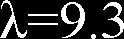
where  ρ—air  density,  R—radius,  Vw—wind  speed, λ—tip speed ratio, λ=ωrR/Vw, ωr—rotor speed, β—pitch angle, and Cp(λ,β)—power coefficient.

(2)

A "one mass" system has been considered to represent the  rotational  dynamics  of  the  gearbox,  wind  turbine  and electrical  generator  [48,  49],  whose  equivalent  moment  of inertia is Jeq. where T, P, and ω represent torque, power and angular  speed,  respectively;  subscripts  g  and  t  are  used  to indicate the variables referring to the generator and the turbine.

fs, p and n are the grid frequency, the number of pole pairs and the gear ratio of the DFIG, respectively. In addition, the DFIG and the rotor side converter (RSC) are both regarded as a single first-order dynamics actuator, with a time constant τC, whose input is the electromagnetic reference torque from the speed control system Tg*.

Tt

Fig. 1 Block diagram of a simplified model of a DFIG-based

Wind Turbine

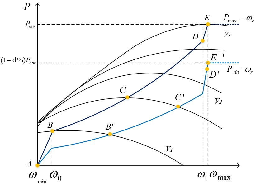
2.1. Maximum Power Point Tracking Controller (MPPT) To  capture  the  maximum  wind  power  by  the  wind turbine, a power reference, Pmax is from the maximum power versus rotor speed (Pmax-ωr) curve that can be represented by (3) and illustrated in Fig. 2 (the solid black line).

(3)

where  kopt  is  the  optimization  constant,  whose  value depends on the physical characteristics of the wind turbine. Concerning Fig. 2, the maximum power curve is divided into four segments according to the rotor speed. The segment A-B corresponds to the starting zone. In segment B-D, known as  the  optimization  zone,  the  rotor  speed  is  adjusted  to  the optimal  speed  with  the  optimal  power  coefficient  Cp(λ,β).

Segments D-E are constant rotor speed zones, and the rotor is almost invariable. After the segment after point E is called the constant power zone, Pmax is constant Pnor.

The intersection point of the capture power versus rotor speed curve (Pm-ωr) and the maximum power curve (Pmax-ωr) is an equilibrium point. After some disturbances, the DFIG-WT automatically  converges  to  the  intersection  point,  where  the captured mechanical power Pm is equal to the optimum power Popt, and the rotor equals ωopt.

A  pitch-angle  controller  is  used  to  prevent  the  rotor speed from exceeding ωmax and keep the output power at the rated value when wind speeds are high.

Fig. 2 Maximum power curve and de-loaded power curve for

2.2. The Traditional Frs For Dfig-Based Wt

The most popular FRS for wind turbines is shown in Fig. 3,  as  in    (and  similar  schemes  in  ,  ).  To realize de-loaded control, a de-loaded power versus rotor speed curve (Pde-ωr) replaces the Pmax-ωr curve. This makes the rotor speed  higher  than  the  optimum  rotor  speed.  The  DFIG-WT operates at a suboptimal point below the maximum power point (reserve a part of the active power). A typical Pde-ωr curve is given in Fig. 2 (the blue line).

An  auxiliary  frequency  controller  (AFC)  is  added  to generate  an  additional  power  ΔPf,  as  expressed  in  (4).  It includes  virtual  inertia  response  and  droop  response.  The inertia  response  is  based  on  the  ROCOF,  while  the  droop response is based on the frequency deviation.

(4)

where Kv and 1/R are the gains of the virtual inertia and droop loops, respectively. The pitch angle control not only prevents the rotor speed from  exceeding  ωmax  but  also  helps  to  realize  de-loaded operation  at  medium  and  high  wind  speeds  area  .

According to wind speed, the de-loaded control can be divided into three areas in , as shown in Fig. 2. (1) Low wind speed area: V1-V2, βde=0, ωr<ωmax; only the speed control loop is used to realize de-loaded control.

(2)  Medium  wind  speed  area:  V2-V3,  βde>0, ωr<ωmax. Both the speed control  loop and  pitch  controller are  used to realize de-loaded control.

(3) High wind area: higher than V3, βde>0, ωr=ωmax, only the pitch controller is used to realize de-loaded control. βde is the de-loaded pitch reference for avoiding overspeed.

The control of the pitch angle is shown in Fig. 3(b). βde is obtained from wind turbine modeling by solving Eq. (5).

(B)

Fig. 3 The commonly used frequency regulation controller for

(5)

where λopt is the optimum tip speed ratio and Cp,max is the maximum wind energy capture factor. λref is the reference tip speed ratio in over speed control, λref=ωmaxR/v, and Cp,rated is the wind energy capture coefficient when operating at rated power.

β0 is the pitch angle reference when the wind turbines operate at the rated power. βde is the de-loaded pitch angle in the de-loaded control  mode.  d’%  is  the  real  de-loaded  ratio  of  the  wind

(6)

where  Popt is  the  reference  power  of  the  wind  turbine under MPPT and Pnor is the rated power. However,  there  are  still  some  shortcomings  for  the traditional frequency regulation scheme.

(1) The gains of AFC are challenging to set because of the compromise of the frequency support performance and wind turbines' stable operation. A large gain can improve the frequency regulation while causing overdeceleration of a DFIG.

Conversely, a small gain can prevent overdeceleration, but it provides  a  limited  contribution  to  frequency  supports.  In addition, for multiple WTGs, the available energy is different because the available energy is determined by the wind turbine characteristics and wind speed. There cannot be a single proper value for all different DFIGs.

(2)  Wind  speed  information  is  required  to  realize de-loaded and frequency support control for the whole section of wind speed. As seen in Fig. 3(b), wind speed information V is necessary for the decision of the wind speed area, calculating the maximum power Popt and the optimum tip speed ratio λopt.

3. The Proposed Frequency Regulation Scheme

To  address  the  limitations  mentioned  above,  a  novel frequency  regulation  scheme  for  de-loaded  wind  turbines  is proposed. The whole control diagram of the proposed scheme is illustrated in Fig. 4.

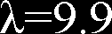
Fig. 4 The Proposed Frequency Regulation Scheme

The  proposed  FRS  includes  two  key  steps.  First,  the de-loaded curve is modified into a droop power curve based on the frequency deviation to provide a droop frequency response.

Second,  the  droop  power  curve  is  further  modified  into  an inertia power curve based on ROCOF to provide both inertia and  droop  frequency  responses.  The  detection  of  dfs/dt  is sensitive to noise and harmonic disturbance. Hence, a washout filter (Tw=0.01)  is used to obtain dfs/dt, as seen in Fig.4.

Then, the power reference PE* can be obtained based on the measurement of the rotor speed ωr. The de-loaded power curve, the droop power curve and the inertia power curve are detailed below.

(7)

where Popt is the maximum available power, Pde is the de-loaded power, and d% is set to 10% in the paper. Similar to the Pmax-ωr curve, the de-loaded curve Pde-ωr

(8)

where  kde is  the  de-loaded  constant  and  Pde  is  the de-loaded power. Noticed that kde does not equal the 0.9kopt. As shown in Fig. 4, for the same wind speed, the rotor speed with 0.9Popt is larger than the optimum rotor speed. By off-line data fitting, it can be obtained that the value of kde with a 10% power reserved ratio is 0.2172. At the maximum rotor speed for the de-loaded power curve, the corresponding wind speed is 10 m/s, instead of 12 m/s for the maximum power curve.

3.2. Droop Power Versus Rotor Curve

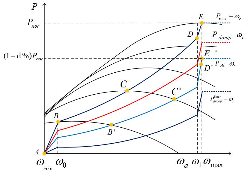
The  droop  power  curve,  Pdroop-ωr,  is  shifted  from  the de-loaded curve (Pde-ωr) to the maximum power curve (Pmax-ωr) based on the frequency deviation.

d% is 10% in this paper, and the droop curve Pdroop-ωr is

(10)

Where  kde80%  is  the  de-loaded  constant  with  an  80% power  reserve  for  the  wind  turbine,  which  to  provide  10% power regulation capability for frequency rise event. kde80% is obtains by off-line data fitting and kde80%=0.1956. Δfmax is the allowable frequency deviation and Δfmax=0.5Hz in this paper.

5

The droop power curve is illustrated in Fig. 5. When the frequency dips, the droop curve moves toward the  Pmax-ωr  curve.  Thus,  the  reference  power  with  the  same rotor  speed  is  larger,  i.e.,  more  active  power  from  the  wind turbine is delivered to the system.

The  droop  response  is  a  minute-term  time  response. Thus, the Pmax-ωr curve is the upper limit of the droop power curve. The additional power from the Pdroop-ωr curve does not exceed the maximum available power.

When  Δfs=0,  Pdroop-ωr  is  the  same  as  the  de-loaded power curve. Otherwise, when the frequency rises, the power curve moves down, and the reference power with the same rotor speed changes to a smaller value. Pdrooplimt -ωr is the lower limit droop curve (as seen in Fig. 5) and is near 80% of the maximum power curve.

Therefore,  the  droop  power  curve  provides  droop frequency  support  for  the  wind  turbine,  similar  to  the  droop response in the traditional auxiliary frequency controller.

Note that there  is always an intersection of the droop power curve and the captured wind power curve (equilibrium point).  This  means  that  the  DFIG  always  converges  to  the equilibrium point in any case. Furthermore, the droop power curve definition does not contain any control gains in (9).

3.3. Inertia Power Curve

Furthermore, to provide inertia supports for the system frequency, the droop power curve, Pdroop-ωr, is further modified into an inertia power versus rotor speed curve, called Pin-ωr, based on the ROCOF (dfs/dt).

In this paper, the inertia power curve is defined in (11) as below.

(11)

where Pupinertial-ωr is the upper limit of the inertia power curve, and Plowerinertial-ωr is the lower limit of the inertia power curve. (dfs/dt)max is the maximum measurement dfs/dt during the frequency event process.

To  obtain  (dfs/dt)  max,  a  latch  is  used  to  store  the maximum value. This means that if a new measurement (dfs/dt) value  is  larger  than  the  old  storage  value,  the  new  value replaces the old storage value. Otherwise, the latch keeps the old storage value.

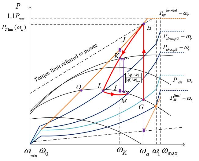
Pupinertial-ωr is defined as in (12), which borrows from . Pupinertial-ωr also shown in Fig. 6.

(12)

PTlim is the torque limit relative to the power curve. ωa is

The Initial Rotor Speed

To avoid the rapid and excessive increase in the output power causing the wind turbine's mechanical torsion, the power limit Plimit and the maximum torque limit Tgmax are often set to 1.1 pu. and 1.07pu .

The minimum torque limit Tgmin are often set to 0. 05pu . The rotor speed increases during the frequency increase event.  Therefore,  the  definition  of  the  Plowerinertial-ωr is  only considered the range of the rotor speed higher than the current rotor ωa . Similarly, the definition of Plowerinertial-ωr is required to prevent  the  speed  rotor  over-accelerating.  the  Pupinertial-ωr  is given in (13), and as the red curve shown in Fig. 6.

Fig. 6 The Inertia Power Curve

To  explain  the  frequency  regulation  proceeding,  a frequency drop event is taken as an example, and the trajectory of operating point during the frequency regulation process is depicted by the red curve in Fig.6.

At  the  initial  time,  'G'  is  assumed  to  be  the  initial operating point located at the de-loaded curve. Δfs and |dfs/dt| are negative values, and dfs/dt quickly drops to the minimum value.  That  is,  |dfs/dt|  reaches  the  maximum  value.  The de-loaded  power  curve  quickly  turns  into  the  upper  limit inertial  curve,  Pupinertial-ωr.  Thus,  the  operating  point  switch from  the  'G'  to  the  point  'H'.  The  wind  turbine  releases  the maximum allowable power for the supported frequency.

Then,  Δfs  and  |dfs/dt|  decreases.  According  to (9),  the droop power curve moves up with Δfs. Meanwhile, the rotor speed ωr decreases because of the extra active power releasing.

'J'  is  the  corresponding  point  with  ωK  located  at  Pupinertial-ωr curve, while 'I' is the corresponding point with ωK located at Pdroop-ωr curve.  Because  of  the  decrease  of  the  dfs/dt (dfs/dt<(dfs/dt)max),  according  to  (11),  the  operating  point moved from 'H' to 'K' (Pin(ωK),ωK). The additional active power from the wind turbine is gradually decreased. Along with dfs/dt approach  to  zero,  the  operating  point  moves  from  the Pupinertial-ωr curve to the droop power curve.

When dfs/dt=0, the frequency reaches the lowest point. At this time, the inertia power curve turns into the droop power curve. The operating point 'K' will turn into 'L' located into the droop power curve Pdroop2-ωr.

Then, the frequency recovery starts. dfs/dt and Δfs are opposite  in  sign.  Unfortunately,  the  inertia  response  is  not beneficial for frequency recovery. Thus, when dfs/dt >0 and Δfs <0,  the  power  curve  maintains  the  droop  power  curve.  The inertial power curve is only enabled when dfs <0 and dfs/dt<0.

As the frequency recovery (Δfs increase), the Pdroop2-ωr curve will move downward to the Pdroop3-ωr curve.  As illustrated in Fig.6, the operating point will move from 'L' to 'M'.

The Pupinertial-ωr curve and the Pm-ωr curve always has an  intersection  (like  'O'  point  in  Fig.6),  which  also  is  an equilibrium point. Only under the extreme situations that dfs/dt keeps the max value (dfs/dt) max, the wind turbine will converge to  this  intersection.  The  rotor  speed  of  this  intersection  still higher  the  minimum  rotor  speed  limit  ωmin.  Practically,  the dfs/dt  will  gradually  reduce  during  the  frequency  regulation process. Hence, the rotor speed always higher than ωmin. during frequency regulation process. Otherwise, the proceeding of the frequency  rise  event  is  similar.  The  proposed  method  can ensure the wind turbine operate among the safe rotor range and prevents overdeceleration.

Noticeably, there are no control gains in (9) - (11). The output power is determined by the current measurement rotor speed and the modified power curve. Thus, unlike the existing scheme's  difficulty  in  choosing  the  proper  control  gains,  the proposed scheme does not have any control gains.

3.4. Pitch Angle Control

As described in the traditional FRS control (Section II. B), in the medium and high wind areas, pitch angle control is necessary  to  add  to  limit  the  rotor  speed  and  help  de-load control.  However,  in  traditional  control,  wind  speed information  is  required  to  decide  the  wind  speed  area  and calculate the value of the compensation pitch βde. However, the inaccurate  wind  speed  measurement  may  be  harmful  to  the control  performance.  Furthermore,  a  complex  calculation  is needed  to  calculate  βde.In  this  paper,  improved  pitch  angle control is designed.

De-Loaded Power Pde

Fig. 7 Pitch angle and de-loaded power at various wind speeds Fig.  7  shows  the  de-loaded  power,  maximum  power pitch angle βm, de-loaded pitch angle βde, and difference angle (between the aforementioned two angles) Δβ versus wind speed.

The maximum power pitch angle remains zero until the wind speed reaches V2. Then, the pitch angle gradually increases to reduce the capture of wind power.

The de-loaded pitch angle remains zero until the wind speed  reaches  V1.  Then,  the  pitch  angle  increases  to  realize de-loaded  control.  During  V1  and  V2,  which  is  called  the medium  wind  speed  area  aforementioned,  both  pitch  angle control and rotor speed control are  used to realize de-loaded control. At wind speeds higher than V2, only the pitch angle is used to realize de-loaded control.

Observing  Δβ in  Fig.  7,  Δβ can  be  divided  into  three segments: a low wind speed area where the wind speed lowers V1, where it is zero; a medium wind speed area during V1 and V2, where  it  is  a  nonlinear  curve;  and  a  high  wind  speed  area, higher than V2, where it has a constant value (nearly 1.6°in this paper).

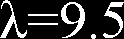
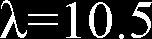
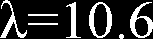
Fig. 8 shows the wind power coefficient Cp versus pitch angle under different tip speed ratios. In the vicinity of λopt (λopt=10.5 in this paper), Cp seems not  to  be  influenced  by  the  different  λ.  Therefore,  the  pitch angle is an almost constant value when Cp is not a considerable reduction.  This  is  the  reason  that  in  the  high  wind  area,  Δβ remains almost constant to realize a certain power reserve.

Linearly fitting the λopt curve to obtain the approximate

Cp= -0.0276Β+ 0.44                           (14)

If  the  DFIG  operates  at  a  10%  power  reserve,  β  will increase by approximately 1.6°.

Wind Power Coefficient Cp

Fig. 8 Wind power coefficient Cp versus pitch angle under differ ent tip speed ratios. Further observing Fig. 7 in the low wind area, the Δβ is zero,  where  the  de-loaded  power  is  below  0.38Pnor;  in  the medium  wind  speed  area,  where  the  de-loaded  power  is between  0.38Pnor  and  0.9Pnor,  the  Δβ  varies  with  de-loaded power.  At  high  wind  speeds,  where  the  de-loaded  power remains at 0.9 Pnor, Δβ remains at a constant value of 1.6°.

Fig. 9 Δβ Versus The De-Loaded Power Curve

The Δβ versus the de-loaded power curve is described in Fig. 9. and the polynomial fitting function given in (15).

(15)

According  to  (15),  Δβ  can  be  obtained  based  on  the de-loaded power Pde. Wind speed information is not required. In  the  medium  and  high  wind  speed  areas,  the  pitch angle must be adjusted to release more or less active power for participation  in  frequency  regulation.  The  improved  pitch control diagram is given in Fig. 10 below.

Fig. 10 The Proposed Pitch Angle Control Scheme

As seen in Fig. 10, Δβ is obtained from equation (15), and  a  simple  linear  method  is  used  to  calculate  the

(16)

Δβ' regulate with the system frequency. when Δf=-Δfmax, Δβ' is equal to 0, and βref = βmppt. When Δf=0, Δβ' is equal to Δβ, and βref=βde (the pitch angle in de-loaded mode).

As  shown  in  the  modified  pitch  angle  control description in Fig. 10, wind speed information is not required. The  pitch  angle  can  help  the  de-loaded  operation  and  the frequency regulation of wind turbines in medium and high wind speed areas.

Matlab/

SIMULINK 2018 Student Suite Version, MathWorks, Natick, MA,  USA  are  carried  out  to  verify  the  proposed  frequency regulation scheme's efficacy.

Fig. 11 shows the single bus model of the small isolated power system used in the paper. It includes static loads, one thermal  plant,  one  hydropower  plant,  and  one  aggregated DFIG-based wind power plant. The total capacity of the power systems is 1250 MW.

S=150Mva

Fig. 11 Single-line diagram of test power system for simulation

(B)

Fig. 12 Governor-based models of conventional power plants Simplified governor-based models from  are used to simulate thermal and hydropower plants (see Fig. 12).

The  droop  characteristics  of  conventional  plant  speed governors  have  been  enabled.  The  values  of  the  most significant parameters are summarized in Appendix table2 and 3.

To  simulate  the  wind  power  plant,  an  equivalent generator with 100 times the nominal power of one DFIG is assumed. The parameters of DFIG-based VSWTs are given in Appendix table.1 The performance of the proposed scheme for DFIG-based  VSWTs  is  compared  to  that  of  MPPT,  the conventional FRS with fixed gain under various wind speeds.

In traditional FRS with fixed gain, Kw is set to 30 and 15, while  1/Rw  is  set  to  24  and  7.  Under  medium  wind  speed conditions, when a larger gain is selected, the inertial control performance of  the DFIG can be effectively improved while ensuring  stable  operation.  In  comparison,  a  smaller  gain  is selected  to  maximize  the  lowest  frequency point  (FN)  while ensuring  stable  operation  of  all  DFIGs  under  low  wind conditions. It is worth noting that the values of large gain and small gain are just an example of traditional FRS. If the system changes, these values should be changed appropriately.

Cases 1, 2, and 3 refer to the constant wind speed in the low wind speed area, the medium wind speed area and the high wind speed area, respectively. In cases 4 and 5, the wind speed is assumed to be reduced at the instant of an event, from 9 to 7.5 m/s for 10 and 1 s, respectively. Case 6 is the random wind speed in low wind area. In all cases, if the rotor speed reaches ωmin, the FRS (not including de-loaded control) are disabled by disconnecting the frequency measurement.

Power,

DFIG-based VSWTs have more difficulty increasing the output power when the frequency dips. Thus, at 60 s, the system load suddenly increases by 0.1 pu and causes a frequency dip event for all cases.

4.1.1 Case1: Low Wind Speed Area

Fig. 13 illustrates the results for a wind speed of 8 m/s in the low wind speed area, where the DFIG-based VSWTs only use overspeed control to realize de-loaded control. 13 shows the result of Case 1.

Deployment In Out-Of-Position Situations

D. Bendjaballah1, A. Bouchoucha1, M. L. Sahli1,2* and J-C. Gelin2

Abstract

Side-impact collisions represent the second greatest cause of fatality in motor vehicle accidents. Side-impact airbags have been installed in recent model year vehicle due to its effectiveness in reducing passengers’ injuries and fatality rates. In meeting these requirements, simulations of folding and deploying airbags are very useful and are widely used. The paper presents a simulation method for the deploying airbags using three materials in different working conditions. Finite element analysis is primarily used to evaluate this concept. In these simulations, the gas flow is described by the conservation laws of mass, momentum, and energy. The numerical results indicate that the FE method in this paper is capable of capturing airbag deploying process accurately.

Keywords: Airbag simulations, Out-of-position, Crash, Modeling, Out-of-position

Background

The passive safety of cars has become a very high prior- ity issue for the automotive industry. Today, there are not only one or two airbags in a car; certain models have ten times more than that. With the increasing usage of airbags, the number of accidents where the airbag itself can cause an injury to the occupant also increases

(Augenstein Et Al. 2003; Gabauer And Gabler 2010;

Audrey et al. 2011). As is well known, safety belts are also now devices designed to provide protection to the users of vehicles during crash events, minimizing the loads necessary to adapt their movement to the move- ment of the car (Freesmeier and Butler 1999; Schmitt et al. 1997). In general, the seat belt is designed to restrain the occupant in the vehicle and prevent the

Occupant From Having Harsh Contacts With Interior

surfaces of the vehicles. The airbag acts to cushion any impact with vehicle structure and has positive internal pressure, which can exert distributed restraining forces over the head and face. As a safety component of auto- mobile, an airbag decreases occupants’ injury likelihood effectively in case of an accident (Ruff et al. 2007). These safety elements can reduce the death rates on the roads, and its protection effects have been widely approved (Crandall et al. 2001; Teru and Ishikawa 2003). With computational tools such as finite element methods designed for dynamic contact problems, crashworthiness simulations can now be used with reliable accuracy to evaluate occupant protection in various collision condi- tions with safety metric/parameters such as acceleration, head injury criteria, intrusion distance, intrusion vel- ocity, and neck forces (neck injury risk or whiplash).

Thus, new types of airbag products are being developed to handle different collision scenarios.

Become Standard Equipment On Most New Passenger

vehicles (Braver and Kyrychenko 2004; Teng et al. 2007; Yoganandan et al. 2007). The airbag cushion is com- posed of a woven fabric which is rapidly inflated during a car crash. The airbag dissipates the passenger’s kinetic energy thereby reducing injury through biaxial stretching of the fabric bag and escaping gas through vents. There- fore, the performance of the airbag is greatly influenced by the mechanical properties of the fabric. Generally, air bags are designed to deploy in a crash that is equivalent to a vehicle crashing into a solid wall at 8 to 14 mph.

Air bags most often deploy when a vehicle collides with another vehicle or with a solid object like a tree. There are various types of airbags: frontal, side-impact, and curtain airbags. In general, the passenger side airbags are usually larger than the driver airbags (see Fig. 1).

Besançon, France

© The Author(s). 2017 Open Access This article is distributed under the terms of the Creative Commons Attribution 4.0 International License (http://creativecommons.org/licenses/by/4.0/), which permits unrestricted use, distribution, and reproduction in any medium, provided you give appropriate credit to the original author(s) and the source, provide a link to the Creative Commons license, and indicate if changes were made.

Bendjaballah et al. International Journal of Mechanical

Doi 10.1186/S40712-016-0070-2

Extensive studies have shown that the airbag deploy- ment in load cases consists of two occupant loading phases: a punch-out effect where the airbag bursts out of its container with the airbag and airbag module cover accelerating towards the occupant and a second loading phase during which the airbag is taking on its deployed shape and volume (membrane-loading effect). Bankdak et al. (2002) developed an experimental airbag test system to study airbag-occupant interactions during close proximity deployment. The results provided insight for simulating the effect of inflation energy and mass flow on target response. Bedard et al. (2002) found that while left-side (driver-side) impacts accounted for only 13.5% of all crashes, the fatality rate among these

Crashes Was 68.3% In Comparison To Front Impact

(48.3%), right-side impact (31.3%), and rear impact (38.4%). These studies underscore the importance of oc- cupant safety during side-impact collisions. In the last years, the current market requested to reduce the time and cost airbag development. In order to achieve this result, virtual simulations play an important role since they allow to minimize the number of experimental tests (Pei et al. 2013; Cao et al. 2014). Several simulation models of airbag were established (Wang et al. 2007). It is feasible to optimize the parameters of airbag deploy- ment using simulation technology. Experimental and numerical studies have quantified injury risks to close- proximity occupants from deploying side airbags. These studies have focused on the prevention of the most ad- verse effects of airbag deployment (Duma et al. 2003).

Other studies have proposed airbag characteristics to minimize particular biomechanical responses (Haland and Pipkorn 1996). In a more recent study, Marklund and Nilsson (2003) compared deformation patterns with experimental data as well as the computational costs associated with three different airbag deployment simu- lation methods; they concluded that the SPH method is relatively inexpensive and produces incremental deform- ation patterns that compare most closely to the experi- mental results. The process of inflation of an airbag is one of the determining factors in saving lives. The duration from the initial impact of the crash to the full inflation of an airbag is about 40 ms, and during this time, the airbag goes from being in a folded state to a fully inflated state, with a high internal pressure. After achieving this state, the airbag begins to deflate, thus providing a nice cushion for the body impacting it.

Ideally, the person in the crash should come into contact with the airbag at this time. In the present study, a large volume passenger side airbag model is developed to handle different collision scenarios. The main aim is evaluate the performance of deploying of passenger side airbag using finite element methods (FEM).

Materials

The tensile specimens were made in different airbags (P: Peugeot, R: Renault, and VW: Volkswagen) with a length of 200 mm long and a width of 40 mm. Table 1 shows the mechanical properties of the airbag.

Tensile Tests

To determine the mechanical properties of the material of airbag used in the test pieces, tensile tests were performed on Lloyd EZ20 universal testing machine in Constantine. These tests were conducted using rect- angular samples. The axial force and axial displacement acquired during a test are converted into stress and the strain in order to be used for the fabric material model.

The continuous recording of the stress-strain data was performed during both the load and unload phases. A minimum of five samples were made in order to check the repeatability of the measurements. All the data was collected by using a PC-based data acquisition system and analyzed by commercial software. The picture frame test device that is made for this study is shown in Fig. 2.

Fig. 1 a Frontal and side airbags. b Oblique view of facet occupant model in sitting posture following airbag deployment (Lim et al. 2014)

0.150

Bendjaballah et al. International Journal of Mechanical and Materials Engineering (2017) 12:12

Page 2 Of 9

Figure 3 shows the stress-strain relationship of the airbag sample under axial tensile loads. The results are showing a linear increase in extension with the increas- ing stresses. This is an expected output and it confirms with the theoretical behavior of a sample subjected to tensile stress. The rupture strain values for different airbags (R/P/VW) were 0.322, 0.441, and 0.472, respect- ively. The measured elastic parameters (i.e., Young’s modulus E and initial yield strength) and Poisson’s ratio are summarized in Table 2. The tensile tests of the woven fabrics can show differences on mechanical prop- erties because woven fabrics can resist in-plane shear loads once the yarn lock-up angle has been reached. The differences of material property on material direction can affect the shape of fully deployed bag (see Fig. 3b).

Theoretical Background

Numerical simulations of airbags use very complex and techniques such as an orthotropic model to identify the mechanical behaviors during the airbag inflation and the fluid mechanics (gas flow) to describe the inflator gas flow (pressure gradient) and improve the representation of the pressures within the airbag. To model the airbag as an orthotropic model, three material constants have to be provided. Assuming a plane stress condition, the

Ð1Þ

where σ is the normal stress and τ is the shear stress, the subscript refers to the principal material directions, i.e., the fill and warp directions. Also, ε and γ are the strain components. The material elastic constants Qij are

Ð2Þ

where E1 and E2 are the Young’s modulus in the fill and wrap directions and G12 is the shear modulus of the fabric material. νij is the Poisson ratio of the material.

The gas exerts a pressure load on the airbag causing it to expand. This expansion puts the airbag under tensile stress lowering the expansion rate. In this study, heat conduction and heat transfer is not taken into account.

Fig. 2 A photograph of Lloyd EZ20 universal testing Fig. 3 Stress versus strain using Lloyd EZ20 machine for a three different airbags at 0° and 90° and b VW airbag test specimens at

Different Angles

Table 2 Physical and mechanical properties of the airbag

Page 3 Of 9

In the deployment of an airbag, an inflator supplies high velocity gas into an airbag causing it to expand rapidly. The gas inside the airbag is assumed to be ideal, to be of constant entropy, and to satisfy the equation of state:

Ð3Þ

Here p, ρ, and e are respectively the pressure, density, and specific internal energy, and γ is the ratio of the heat capacities of the gas. The gas flow is described by the conservation laws for mass, momentum, and energy that

Ð4Þ

here, V is a volume, A is the boundary of this volume,

N Is The Normal Vector Along The Surface A, And U

denotes the velocity vector in the volume. Applying Bernoulli’s equation in the case of an ideal gas with

Ð5Þ

Here, the subscript ex denotes quantities at the throat of the tube. Furthermore u, p, and ρ denote the quan- tities inside that part of the tube that is supplying mass.

Materials And Boundary Conditions

The airbag system mainly consists of three parts: the airbag itself, the inflator unit, and the crash sensor or diagnostic unit. Thus, to study the behavior of the airbag using FE simulations, we need to have an FE model of the airbag in the folded position. A FE model of the airbag was used to simulate the test condition as shown in Fig. 5. LS-DYNA® material model FABRIC (MAT_34) is used to simulate the airbag material. It is a variation of the layered orthotropic material model. Additionally, in the LS-DYNA® material model, fabric leakage can be accounted for. However, for this CAB material, the leak- age is almost negligible and therefore no leakage is specified. The mechanical properties can be determined from the physical test. Typical material properties for airbag fabrics are taken as given in Chawla et al. (2004a) (Table 3). These properties are used to simulate inflation process of airbag (see Table 1). The car dashboard is modeled as the rectangular thin plate using a MAT_RI-

Gid Material, And The Degrees Of Freedom Are Con-

strained in all the directions. The similar properties of thermoplastic polymer are assigned for contact purposes. The porosity of the fabric is assumed zero. The nitro- gen gas is taken for inflating the airbag. Properties of nitrogen gas and initial bag conditions are shown in Table 4. The example on which we perform the study is a typical passenger side airbag. The geometric de- tails have been measured from a commercially avail- able airbag. The initial state of the airbag is a closed rectangular whose sides are to be finished to 482 × 635 mm2 and is shown in Fig. 4.

Table 3 Material properties of airbag and rigid plate used in FE

–

Table 4 Initial values used for FE simulation of the swelling of

3.33 × 10−4

Fig. 4 The initial airbag geometry in the form of a rectangular Bendjaballah et al. International Journal of Mechanical and Materials Engineering (2017) 12:12

Related Journal Articles & DOI Links

Selected peer-reviewed publications relevant to 12 Lead ECG Acquisition. Click the DOI to access the full paper (may require institutional access).

Why Choose Us?

Bangalore guidance for robotics, Spectre and autonomous systems projects.