Autonomous Underwater Vehicle

Ntroduction

About 70% of the surface of the Earth is covered by oceans, and the ocean space represents a vast chamber of natural resources. In order to explore and utilize these resources, humankind depends on developing and employing underwater vehicles, not least unmanned underwater vehicles (UUVs). Today, UUVs encompass remotely operated vehicles (ROVs) and autonomous underwater vehicles (AUVs).

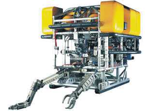
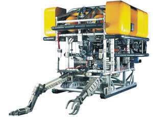
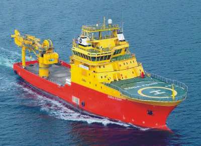
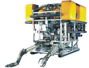
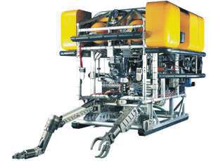
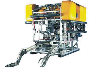
The first ROVs were built in the 1950s, put into commercial use in the 1980s, and are mostly used today by the offshore oil and gas industry to carry out inspection and intervention operations at subsea installations (Antonelli et al. 2008). These vehicles are teleoperated by connection to a surface vessel through an umbilical cable that provides them with power and telemetry. In particular, the dependence on a tether represents a considerable challenge for ROV deepwater operations (Whitcomb 2000).

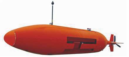
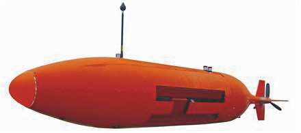
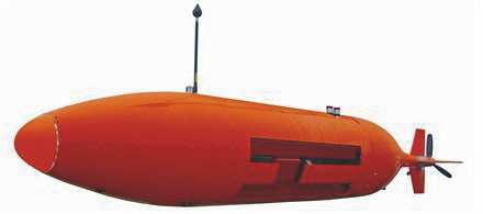
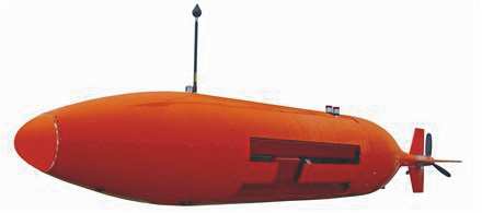
On the other hand, AUVs are free-swimming vehicles that rely on their own energy supply. The first AUVs were built in the 1970s, put into commercial use in the 1990s, and today are mostly used for scientific, commercial, and military mapping and survey tasks (Blidberg 2001). Developed in cooperation between Kongsberg Maritime and the Norwegian Defence Research Establishment, the HUGIN series represents the most commercially successful AUV series on the world market today (Hagen et al. 2003). HUGIN vehicles have been employed for commercial applications since 1997 and for military applications since 2001.

The workhorse HUGIN 3000 has an impressive 60 hours endurance at 4 knots speed with payload sensors running. Currently, the main challenges for AUVs encompass endurance, navigation, communication, and autonomy issues.

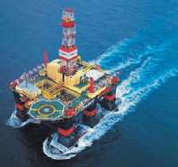
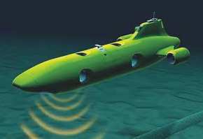
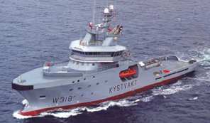
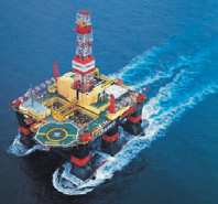
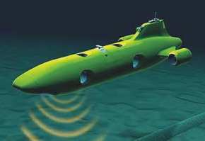
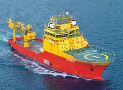
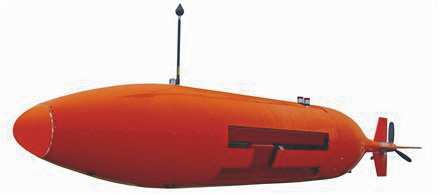
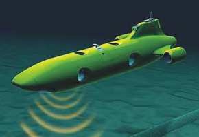
Traditionally, ROVs and AUVs have been assigned different tasks due to different strengths and weaknesses, see Fig. 1. In the future, hybrid ROV/AUV designs are expected to bridge the gap between these two main UUV types, utilizing the best of both worlds (Wernli 2000).

Regarding motion control research for UUVs, Craven et al. (1998) give an overview of modern control approaches with an emphasis on artificial intelligence techniques; Roberts & Sutton (2006) treat guidance, navigation, and control issues for unmanned marine vehicles with an emphasis on underwater vehicles; while Antonelli et al. (2008) present a state-of-the-

Open Access Database Www.Intechweb.Org

Source: Underwater Vehicles, Book edited by: Alexander V. Inzartsev,

Underwater Vehicles

Fig. 1. The two traditional types of UUVs: ROVs and AUVs. These vehicles have different designs and perform different operations in different parts of the speed regime An essential quality for free-swimming underwater vehicles like AUVs is their ability to maneuver accurately in the ocean space. Motion control is a fundamental enabling technology for such a quality, and every motion control system requires a guidance component. This guidance requirement serves as the main motivation for this work, whose aim is to provide a convenient overview of guidance laws applicable to motion control of AUVs. An extension of (Breivik & Fossen 2008), the exposition is deliberately kept at a basic level to make it accessible for a wide audience. Details and proofs can be found in the

Guidance

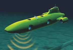
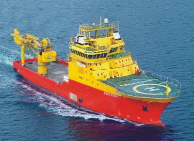
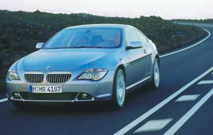
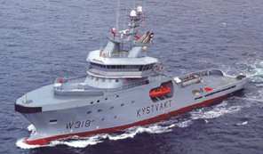
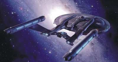
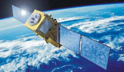
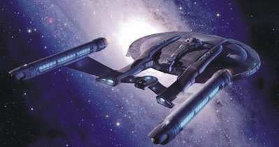
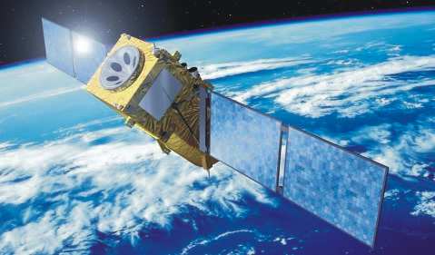
According to Shneydor (1998), guidance is defined as: The process for guiding the path of an object towards a given point, which in general may be moving. Also, the father of inertial navigation, Charles Stark Draper, states in (Draper 1971) that: Guidance depends upon fundamental principles and involves devices that are similar for vehicles moving on land, on water, under water, in air, beyond the atmosphere within the gravitational field of earth and in space outside this field, see Fig. 2. Thus, guidance represents a basic methodology concerned with the transient motion behavior associated with the achievement of motion control objectives.

The most rich and mature literature on guidance is probably found within the guided missile community. In one of the earliest texts on the subject (Locke 1955), a guided missile is defined as: A space-traversing unmanned vehicle which carries within itself the means for controlling its flight path. Today, most people would probably think about unmanned aerial vehicles (UAVs) when hearing this definition. However, guided missiles have been operational since World War II (Spearman 1978), and thus organized research on guidance theory has been conducted almost as long as organized research on control theory. The continuous progress in missile hardware and software technology has made increasingly advanced guidance concepts feasible for implementation. Today, missile guidance theory encompass a broad spectrum of guidance laws, namely: classical guidance laws; optimal guidance laws; guidance laws based on fuzzy logic and neural network theory; differential- geometric guidance laws; and guidance laws based on differential game theory.

Guidance Laws For Autonomous Underwater Vehicles

Fig. 2. Fundamental guidance principles apply from subsea to space As already mentioned, a classical text on missile guidance concepts is (Locke 1955), while more recent work include (Lin 1991), (Shneydor 1998), (Zarchan 2002), (Siouris 2004), and (Yanushevsky 2008). Relevant survey papers include (Pastrick et al. 1981), (Cloutier et al.

1989), (Lin & Su 2000), and (White & Tsourdos 2001). Also, very interesting personal accounts of the guided missile development during and after World War II can be found in (Haeussermann 1981), (Battin 1982), and (Fossier 1984), while MacKenzie (1990) and Westrum (1999) put the development of guided missile technology into a larger perspective.

The fundamental nature and diverse applicability of guidance principles can be further illustrated through a couple of examples. In nature, some predators are able to conceal their pursuit of prey by resorting to so-called motion camouflage techniques (Mizutani et al.

2003). They adjust their movement according to their prey so that the prey perceive them as stationary objects in the environment. These predators take advantage of the fact that some creatures detect the lateral motion component relative to the predator-prey line of sight far better than the longitudinal component. Hence, approaching predators can appear stationary to such prey by minimizing the relative lateral motion, only changing in size when closing in for the kill. Interestingly, this behavior can be directly related to the classical guidance laws from the missile literature (Justh & Krishnaprasad 2006). Also, such guidance laws have been successfully applied since the early 1990s to avoid computationally- demanding optimization methods associated with motion planning for robot manipulators operating in dynamic environments (Piccardo & Honderd 1991).

Otion Control Fundamentals

This section reviews some basic motion control concepts, including operating spaces, vehicle actuation properties, motion control scenarios, as well as the motion control hierarchy. It concludes with some preliminaries.

Operating Spaces

It is useful to distinguish between different types of operating spaces when considering vehicle motion control, especially since such characterizations enable purposeful definitions of various motion control scenarios. The two most fundamental operating spaces to consider are the work space and the configuration space.

The work space, also known as the operational space (Sciavicco & Siciliano 2002), represents the physical space (environment) in which a vehicle moves. For a car, the work space is 2- dimensional (planar position), while it is 3-dimensional (spatial position) for an aircraft.

Thus, the work space is a position space which is common for all vehicles of the same type. The configuration space, also known as the joint space (Sciavicco & Siciliano 2002), is constituted by the set of variables sufficient to specify all points of a (rigid-body) vehicle in the work space (LaValle 2006). Thus, the configuration of a car is given by its planar position and orientation, while the configuration of an aircraft is given by its spatial position and attitude.

Ehicle Actuation Properties

Every variable associated with the configuration of a vehicle is called a degree of freedom (DOF). Hence, a car has 3 degrees of freedom, while an aircraft has 6 degrees of freedom. The type, amount, and distribution of vehicle thrust devices and control surfaces, hereafter commonly referred to as actuators, determine the actuation property of a vehicle. We mainly distinguish between two qualitatively different actuation properties, namely full actuation and underactuation. A fully actuated vehicle is able to independently control all its DOFs simultaneously, while an underactuated vehicle is not. Thus, an underactuated vehicle is generally unable to achieve arbitrary tasks in its configuration space. However, it will be able to achieve tasks in the work space as long as it can freely project its main thrust in this space, e.g., through a combination of thrust and attitude control. In fact, this principle is the mode by which most vehicles that move through a fluid operate, from missiles to ships.

Even if these vehicles had the ability to roam the work space with an arbitrary attitude, this option would represent the least energy-efficient alternative.

Otion Control Scenarios

In the traditional control literature, motion control scenarios are typically divided into the following categories: point stabilization, trajectory tracking, and path following. More recently, the concept of maneuvering has been added to the fold as a means to bridge the gap between trajectory tracking and path following (Skjetne et al. 2004). These scenarios are often defined by motion control objectives that are given as configuration-space tasks, which are best suited for fully actuated vehicles. Also, the scenarios typically involve desired motion that has been defined apriori in some sense. Little seems to be reported about tracking of target points for which only instantaneous motion information is available.

However, in this work, both apriori and non-apriori scenarios are considered, and all the motion control objectives are given as work-space tasks. Thus, the scenarios cover more

Guidance Laws For Autonomous Underwater Vehicles

broadly, and are also suited for underactuated vehicles. The considered scenarios are defined in the following. The control objective of a target-tracking scenario is to track the motion of a target that is either stationary (analogous to point stabilization) or that moves such that only its instantaneous motion is known, i.e., such that no information about the future target motion is available. Thus, in this case it is impossible to separate the spatio-temporal constraint associated with the target into two separate constraints.

In contrast, the control objective of a path-following scenario is to follow a predefined path, which only involves a spatial constraint. No restrictions are placed on the temporal propagation along the path.

However, the control objective of a path-tracking scenario is to track a target that moves along a predefined path (analogous to trajectory tracking). Consequently, it is possible to separate the target-related spatio-temporal constraint into two separate constraints. Still, this scenario can be viewed as a target-tracking scenario and handled with target-tracking methods, thus disregarding any apriori path information that is available.

Finally, the control objective of a path-maneuvering scenario is to employ knowledge about vehicle maneuverability to feasibly negotiate (or somehow optimize the negotiation of) a predefined path. As such, path maneuvering represents a subset of path following, but is less constrained than path tracking since spatial constraints always take precedence over temporal constraints. Path-maneuvering methods can also be used to handle path-tracking scenarios.

Otion Control Hierarchy

A vehicle motion control system can be conceptualized to involve at least three levels of control in a hierarchical structure, see Fig. 3. This figure illustrates the typical components of a marine motion control system, encompassing strategic, tactical, and execution levels of control (Valavanis et al. 1997). All the involved building blocks represent autonomy- enabling technology, but more instrumentation and additional control levels are required to attain fully autonomous operation. An example involves collision avoidance functionality, which demands additional sense and avoid components.

This work is mainly concerned with the highest (strategic) control level of Fig. 3. Termed the kinematic control level, it is responsible for prescribing vehicle velocity commands needed to achieve motion control objectives in the work space. Thus, in this work, kinematic control is equivalent to work-space control, and kinematic controllers are referred to as guidance laws.

This level purely considers the geometrical aspects of motion, without reference to the forces and moments that generate such motion. Next, the intermediate (tactical) level encompass kinetic controllers, which do consider how forces and moments generate vehicle motion. These controllers are typically designed by model-based methods, and must handle both parametric uncertainties and environmental disturbances. For underactuated vehicles, they must actively employ the vehicle attitude as a means to adhere to the velocities ordered by the guidance module. The intermediate control level also contains a control allocation block which distributes the kinetic control commands among the various vehicle actuators.

Finally, the lowest (execution) level is constituted by the individual actuator controllers, which ensure that the actuators behave as requested by the intermediate control module, and ultimately that the vehicle moves as prescribed by the guidance laws.

Underwater Vehicles

Fig. 3. The motion control hierarchy of a marine surface vessel

Preliminaries

In the missile literature, guidance laws are typically synonymous with steering laws, assuming that the speed is constant. In this work, guidance laws are either directly prescribed as velocity assignments or partitioned into separate speed and steering laws.

The guidance laws are first introduced in a 2-dimensional framework, where a kinematic

P$

R , stated relative to some stationary reference frame. Since most of the AUVs of today are of the survey type, they do not need to perform spatially coupled maneuvers, but typically execute temporally separated planar maneuvers either in the horizontal plane or the vertical plane. Thus, Section 3 and 4 are relevant for such applications. Similar considerations justify the work reported in (Healey & Lienard 1993), (Caccia et al. 2000), and (Lapierre et al. 2003).

In Section 5, the planar methods are extended to a 3-dimensional framework, where a kinematic vehicle is represented by its spatial position

V

. Results on spatially coupled motion control of AUVs can be found in (Encarnação & Pascoal 2000), (Do & Pan 2003), (Aguiar & Hespanha 2004), (Breivik & Fossen 2005a), (Børhaug & Pettersen 2006), and (Refsnes et al. 2008).

Finally, note that all the illustrations of guidance principles employ the marine convention of a right-handed coordinate system whose z-axis points down.

Guidance Laws For Target Tracking

In this section, guidance laws for target tracking are presented. The material is adapted from (Breivik & Fossen 2007).

P

is either stationary or moving by a (non-zero and bounded) velocity

P

. Concerning tracking of moving targets, the missile guidance community probably has the most comprehensive experience. They commonly refer to the object that is supposed to destroy another object as either a missile, an interceptor, or a pursuer. Conversely, the threatened object is typically called a target or an evader. Here, the designations interceptor and target will be used.

An interceptor typically undergoes 3 phases during its operation; a launch phase, a midcourse phase, and a terminal phase. The greatest accuracy demand is associated with the terminal phase, where the interceptor guidance system must compensate for the accumulated errors from the previous phases to achieve a smallest possible final miss distance to the target. Thus, 3 terminal guidance strategies will be presented in the following, namely line of sight, pure pursuit, and constant bearing. The associated geometric principles are illustrated in Fig. 4.

Note that while the main objective of a guided missile is to hit (and destroy) a physical target in finite time, we recognize the analogy of hitting (converging to) a virtual target asymptotically, i.e., the concept of asymptotic interception, as stated in (1).

Ine Of Sight Guidance

Line of sight (LOS) guidance is classified as a so-called three-point guidance scheme since it involves a (typically stationary) reference point in addition to the interceptor and the target. The LOS denotation stems from the fact that the interceptor is supposed to achieve an intercept by constraining its motion along the line of sight between the reference point and the target. LOS guidance has typically been employed for surface-to-air missiles, often mechanized by a ground station which illuminates the target with a beam that the guided missile is supposed to ride, also known as beam-rider guidance. The LOS guidance principle is illustrated in Fig. 4, where the associated velocity command is represented by a vector pointing to the left of the target.

Pure Pursuit Guidance

Pure pursuit (PP) guidance belongs to the so-called two-point guidance schemes, where only the interceptor and the target are considered in the engagement geometry. Simply put, the interceptor is supposed to align its velocity along the line of sight between the interceptor and the target. This strategy is equivalent to a predator chasing a prey in the animal world, and very often results in a tail chase. PP guidance has typically been employed for air-to-surface missiles. The PP guidance principle is represented in Fig. 4 by a vector pointing directly at the target.

Underwater Vehicles

Fig. 4. The interceptor velocity commands that are associated with the classical guidance principles line of sight (LOS), pure pursuit (PP), and constant bearing (CB) Deviated pursuit guidance is a variant of PP guidance where the velocity of the interceptor is supposed to lead the interceptor-target line of sight by a constant angle in the direction of the target movement. An equivalent term is fixed-lead navigation.

Onstant Bearing Guidance

Constant bearing (CB) guidance is also a two-point guidance scheme, with the same engagement geometry as PP guidance. However, in a CB engagement, the interceptor is supposed to align the relative interceptor-target velocity along the line of sight between the interceptor and the target. This goal is equivalent to reducing the LOS rotation rate to zero such that the interceptor perceives the target at a constant bearing, closing in on a direct collision course. CB guidance is often referred to as parallel navigation, and has typically been employed for air-to-air missiles. Also, the CB rule has been used for centuries by mariners to avoid collisions at sea; steering away from a situation where another vessel approaches at a constant bearing. Thus, guidance principles can just as well be applied to avoid collisions as to achieve them. The CB guidance principle is indicated in Fig. 4 by a vector pointing to the right of the target.

The most common method of implementing CB guidance is to make the rotation rate of the interceptor velocity directly proportional to the rotation rate of the interceptor-target LOS, which is widely known as proportional navigation (PN).

CB guidance can also be implemented through the direct velocity assignment

(3)

is the line of sight vector between the interceptor and the target,

A,Max > 0

specifies the maximum approach speed toward the target, and Δ #p > 0 affects the transient interceptor-target rendezvous behavior. Note that CB guidance becomes equal to PP guidance for a stationary target, i.e., the basic difference between the two guidance schemes is whether the target velocity is used as a kinematic feedforward or not.

Returning to the example on motion camouflage, it seems that two main strategies are in use; camouflage against an object close by and camouflage against an object at infinity. The first strategy clearly corresponds to LOS guidance, while the second strategy equals CB guidance since it entails a non-rotating predator-prey line of sight.

Guidance Laws For Path Scenarios

In this section, guidance laws for different path scenarios are considered, including path following, path tracking, and path maneuvering. Specifically, the guidance laws are composed of speed and steering laws, which can be combined in various ways to achieve different motion control objectives. The speed is denoted

∈−

. Path following is ensured by proper assignments to χ( )t as long as

Since The

scenario only involves a spatial constraint, while the spatio-temporal path-tracking and path-maneuvering scenarios both require explicit speed laws in addition to the steering laws. The following material is adapted from (Breivik & Fossen 2004a), (Breivik & Fossen 2005b), and (Breivik et al. 2008).

Steering Laws For Straight Lines

Consider a straight-line path implicitly defined by two waypoints through which it passes.

P

, respectively. Also, consider a path-fixed reference frame with origin in

Relative To The X-Axis Of The Stationary

reference frame. Hence, the coordinates of the kinematic vehicle in the path-fixed reference

( )

e t , see Fig. 5. For path-following purposes, only the cross-track error is relevant since

Underwater Vehicles

Fig. 5. The main variables associated with steering laws for straight-line paths

E T

means that the vehicle has converged to the straight line. Expanding (5), the cross-

(7)

and the associated control objective for straight-line path following becomes

(8)

In the following, two steering laws that ensure stabilization of ( )

E T To The Origin Will Be

presented. The first method is used in ship motion control systems (Fossen 2002), and will be referred to as enclosure-based steering. The second method is called lookahead-based steering, and has links to the classical guidance principles from the missile literature. The two steering methods essentially operate by the same principle, but as will be made clear, the lookahead-based scheme has several advantages over the enclosure-based approach.

F The Circle Radius Is Chosen Sufficiently

large, the circle will intersect the straight line at two points. The enclosure-based strategy for

( )

e t to zero is then to direct the velocity toward the intersection point that corresponds to the desired direction of travel, which is implicitly defined by the sequence in which the waypoints are ordered. Such a solution involves directly assigning

P

represents the intersection point of interest. In order to

P

(two unknowns), the following two equations must be solved

(11)

where (10) represents the theorem of Pythagoras, while (11) states that the slope of the line between the two waypoints is constant. These equations are solved in the following, temporarily dropping the time dependence of the variables for notational convenience.

Denote the difference between the x- and y-position of the two waypoints as

Y

y , respectively. The equations are first solved analytically assuming that

Y

. For simplicity and brevity in the calculations to follow,

(16)

which is a standard, analytically-solvable second order equation. Then, denote

Ookahead-Based Steering

Here, the steering assignment is separated into two parts

(21)

is a velocity-path relative angle which ensures that the velocity is directed toward a point on the path that is located a lookahead distance Δ > 0 ahead of the direct projection of

Onto

the path (Papoulias 1991), see Fig. 5. As can be immediately noticed, this lookahead-based steering scheme is less computationally intensive than the enclosure-based approach. It is also valid for all cross- track errors, whereas the enclosure-based strategy requires

(22)

which means that the enclosure-based approach corresponds to a lookahead-based scheme

E T

). Only lookahead-based steering will be considered in the following.

Piecewise Linear Paths

If a path is made up of n straight-line segments connected by n+1 waypoints, a strategy must be employed to purposefully switch between these segments as they are traversed. In (Fossen 2002), it is suggested to associate a so-called circle of acceptance with each

P

has entered the waypoint-enclosing circle. Note that for the enclosure-based approach, such a switching criterion entails the additional (conservative)

R

. A perhaps more suitable switching criterion solely involves the along-track distance ( )

S T ,

such that if the total along-track distance between waypoints

(24)

which is similar to (23), but has the advantage that p(t) does not need to enter the waypoint- enclosing circle for a switch to occur, i.e., no restrictions are put on the cross-track error. Thus, if no intrinsic value is associated with visiting the waypoints, and their only purpose is to implicitly define a piecewise linear path, there is no reason to apply the circle-of- acceptance switching criterion (23).

Subsequently, Consider

a path-fixed reference frame with origin at the direct projection of

Underwater Vehicles

Fig. 6. The main variables associated with steering for circles path, see Fig. The x-axis of this reference frame has been rotated a positive angle (relative

To Clockwise

motion. Hence, χp becomes time-varying for circular (curved) motion, as opposed to the constant χp associated with straight lines (20). Also, note that (26) is undefined for

P ,

i.e., when the kinematic vehicle is located at the circle center. In this case, any projection of

P

onto the circular path is valid, but in practice this problem can be alleviated by, e.g., purposefully choosing χ c( )t based on the motion of ( )t

P

. Since the path-following control objective for circles is identical to (8), lookahead-based steering can be employed, implemented by using (19) with (25) instead of (20), and

Authors:

Peder EZ Larson 1, 2,* , Jenna ML Bernard1, James A Bankson 3, Nikolaj Bøgh 4, Robert A Bok1, Albert P. Chen 5, Charles H Cunningham 6,7, Jeremy Gordon1, Jan-Bernd Hövener 8, Christoffer Laustsen 4, Dirk Mayer 9,10, Mary A McLean11 12, Franz Schilling13, James Slater1, Jean-Luc Vanderheyden5, 14, Cornelius von Morze 15, Daniel B Vigneron1, 2, Duan Xu1, 2, and the HP 13C

94143, Usa.

Denmark. 5 GE Healthcare, Menlo Park, California, USA. 6 Physical Sciences, Sunnybrook Research Institute, Toronto, Ontario, Canada.

8 Section Biomedical Imaging, Molecular Imaging North Competence Center (MOIN CC), Medicine, Baltimore, MD, USA. Cambridge, United Kingdom.

14Jlvmi Consulting Llc, Dousman, Wi, Usa

#See Acknowledgements for a list of all HP 13C MRI Consensus Group Members This work was supported by the ISMRM Hyperpolarized Media MR Study Group, the ISMRM Hyperpolarization Methods & Equipment Study Group, and the Hyperpolarized MRI Technology Resource Center (NIH/NIBIB grant P41EB013598).

Abstract

MRI with hyperpolarized (HP) 13C agents, also known as HP 13C MRI, can measure processes such as localized metabolism that is altered in numerous cancers, liver, heart, kidney diseases, and more. It has been translated into human studies during the past 10 years, with recent rapid growth in studies largely based on increasing availability of hyperpolarized agent preparation methods suitable for use in humans. This paper aims to capture the current successful practices for HP MRI human studies with [1-13C]pyruvate - by far the most commonly used agent, which sits at a key metabolic junction in glycolysis. The paper is divided into four major topic areas: (1) HP 13C-pyruvate preparation, (2) MRI system setup and calibrations, (3) data acquisition and image reconstruction, and (4) data analysis and quantification. In each area, we identified the key components for a successful study, summarized both published studies and current practices, and discuss evidence gaps, strengths, and limitations. This paper is the output of the “HP 13C MRI Consensus Group” as well as the ISMRM Hyperpolarized Media MR and Hyperpolarized Methods & Equipment study groups. It further aims to provide a comprehensive reference for future consensus building as the field continues to advance human studies with this metabolic imaging modality.

Keywords: Hyperpolarized MRI, metabolic imaging, carbon-13, pyruvate, dissolution dynamic

Introduction

MRI with hyperpolarized 13C agents, also known as hyperpolarized (HP) 13C MRI, has shown great potential as a novel imaging modality, particularly for its ability to probe metabolic processes in real time. The first human studies with HP [1-13C]pyruvate were performed in 2011 in prostate cancer patients (1).

Since then, there have been over 60 papers published with imaging results of human subjects from 13 different sites, with applications including prostate cancer, brain tumors, breast cancer, kidney cancer, pancreatic cancer, metastatic disease, liver disease, ischemic heart disease, diabetes and cardiomyopathies. The vast majority of these studies used [1-13C]pyruvate (1–63), where [2-13C]pyruvate (64) and 13C-urea (56) have been demonstrated too.

As clinical HP 13C MRI advances, there is a growing need to build consensus for best practices, which are critical for comparing data across sites, performing multi-site trials,deploying methods to new sites, partnering with vendors, and potentially for obtaining broader regulatory approvals.

In March 2022, we initiated an effort to build consensus within the HP 13C MRI community with this opportunity in mind, and it was greeted with strong enthusiasm. The “HP 13C MRI Consensus Group”, containing over 55 members from 27 sites, identified the area of greatest need and opportunity for consensus building to be HP [1-13C]pyruvate human

●

Pyruvate is the most mature and widely used HP agent and has the most significant translational evidence emphasizing the potential clinical impact.

●

Clinical trials, particularly multi-site trials, have the strongest need for consensus methods to ensure that data can be combined across sites. This work is a Position Paper for which the goal is to describe current successful practices and study methods for HP [1-13C]pyruvate human studies along with justification to support those practices. This is divided into four major topic areas: (1) HP 13C-pyruvate preparation, (2) MRI system setup and calibrations, (3) data acquisition and image reconstruction, and (4) data analysis and quantification (Fig. 1). The current successful practices and study methods include a literature review of published peer-reviewed journal papers showing human HP [1-13C]pyruvate study data, up to September 2022 (1–63), as well as new unpublished information from surveys of HP 13C study sites. Based on this information, we also highlight the evidence gaps, strengths, and limitations of current practices which are summarized at the end of each section.

Figure 1: Illustration of the HP 13C MRI human study process, including the 4 major areas covered in this paper: Hyperpolarized 13C-pyruvate preparation, MRI system setup and calibration, Acquisition and Reconstruction, and Data Analysis and Quantification.

Figure 2: Anatomical targets of HP [1-13C]pyruvate MRI human studies published up to September 2022.

Hyperpolarized 13C-Pyruvate Preparation

This section covers the processes for creating the HP agent, 13C pyruvate, and will include many aspects and considerations that are needed to safely and effectively prepare doses for metabolic imaging studies in human subjects. These include material, personnel, equipment and facility, fluid path preparation, quality control, and release.

It is helpful to understand that the specifications of a dose of 13C pyruvate suitable for in vivo MR HP metabolic imaging were shaped in part by early preclinical studies performed by GE HealthCare summarized in Ref. (65). In short, the safety of the two novel drug components, 13C pyruvate and the electron paramagnetic agent (EPA) AH111501, were demonstrated in those studies. The more precise formulation of the dose suitable for human use was then determined from clinical studies (66) that included two Phase 1 clinical trials in young and elderly healthy volunteers without hyperpolarization of the 13C nuclei and another Phase 1/2a dose escalation and imaging feasibility study with HP 13C pyruvate in 31 prostate cancer patients at the With the exception of the first HP 13C imaging clinical trial, which utilized a prototype device in a cleanroom (1), all HP 13C studies performed in humans to date have utilized the SPINlab polarizer (manufactured by GE HealthCare). Consequently all doses of the HP 13C pyruvate delivered by SPINlab have been produced using the “SPINlab Pharmacy Kit” that serves as the container-closure system for the various drug components (13C pyruvic acid and EPA mixture, dissolution medium, and neutralization and dilution medium) during sample polarization, dissolution and quality control (QC) processes. Thus many aspects of the HP sample preparation considerations discussed below are related to the SPINlab instrument and the consumables designed to be used with it (67).

General Considerations

While more than 860 patients or healthy subjects having been injected with HP 13C pyruvate as of January 2022 without reports of any serious adverse events (68), HP 13C pyruvate injection remains an investigational MR contrast agent and can only be administered by those with Investigational New Drug (IND) exemption from the Food and Drug Administration (FDA) in the USA, a Clinical Trial Application (CTA) in Canada, approval from National Research Ethics Committee Services in the UK, or approval from the relevant local regulatory body. Thus, methods and processes involved to produce a dose should have patient safety as the first priority. Since utilizing dissolution dynamic nuclear polarization (dissolution-DNP) for human use is still a relatively new development, there are no existing published regulatory guidelines specifically for this method.

There are two major production styles that determine how various sites approach the agent preparation. In the US, the most common approach is to rely on a sterilizing filter (“Terminal Sterilization”) to ensure sterility of the final product, akin to PET tracer production, where a starting molecule with a radioisotope is processed using various other ingredients to make the final, desired and injectable contrast agent within a necessarily short amount of time (69). For these sites, sterilization of the components and accessories upstream of this filter are not required, although many of them were manufactured and tested following Good Manufacturing Practice (GMP) or Good Laboratory Practice (GLP) requirements. The filling process is usually performed under an ISO 5 laminar flow hood, but a clean room or an isolator is not required.

This approach is typically accompanied by testing the integrity of the sterilizing filter prior to release of the dose for injection. Typically, post release endotoxin and sterility tests are performed using an aliquot reserved from each released dose.

In the UK and EU, the most common approach is to more-closely follow sterile pharmaceutical compounding guidelines (70), where all components and ingredients are required to be sterile or manufactured under GMP guidelines and are assembled and filled within a clean room environment or an isolator system (“Sterile Preparation”). Typically a batch of Pharmacy Kits for HP 13C pyruvate injection are prepared together. The sterility of the final dose is also ensured by batch validation testing, in addition to the sterility of the ingredients and the sterile compounding process. The endotoxin and sterility testing are performed for the process validation but are not performed for each injected dose.

Some institutions fill and assemble the Pharmacy Kit required for a specific study on the same day or the day prior to polarization, dissolution, and patient administration, but others have also demonstrated the feasibility of preparing a batch of kits, keeping them in a -20ºC freezer and using them over a period of a few months.

Beyond the obvious requirements that the process and the facility has to ultimately produce a dose that is safe to inject into a human, regulatory authorities will also focus on the question “Are you in control of your processes?”. To be in control of your process requires an in-depth and broad understanding of all processes involved in pre, post, and during the production process.

Personnel

It is typical and may be required to have licensed personnel involved in the production process depending on local regulations.Typically a pharmacist, radiopharmacist or other similarly qualified person (QP), in charge of the facility where the Pharmacy Kit filling and preparation is taking place, is responsible for the overall process and the release of the injectable dose.

Qualified cleanroom technicians are often involved in the Pharmacy Kit filling under the supervision of the pharmacist or QP. As is required for pharmaceutical compounding or PET tracer production, training requirements and training records for all personnel need to be maintained and available for audit by the FDA or equivalent.

Equipment And Facility

The facility and all equipment need to have standard operating procedures (SOPs) that describe how equipment is used, maintained, and calibrated to comply with relevant legislation. Currently, almost all the filling of the Pharmacy Kit takes place within a compounding laminar flow hood or isolator (typically ISO 5). At some sites, the filling is conducted within a cleanroom, while at others, it is conducted in a dedicated non-cleanroom space, reflecting differences in cleanroom approach and specifications between regulators worldwide (71). Some equipment or facilities, such as the compounding hood or cleanroom, may require external certified laboratories for testing.

Material Handling

Material handling guidelines (69,70) require SOPs detailing a system to track all of the materials involved in the HP production process for a particular patient dose, similar to current good manufacturing practice (cGMP) requirements for material handling for drug compounding. This includes acceptance standards, storage conditions, amount used in the patient dose for each ingredient and materials used in the assembly of the fluid path and Pharmacy Kit. Currently some users choose to open and inspect and sometimes modify the Pharmacy Kits upon arrival, but some users keep them in the sealed packaging until they are required for dose preparation.

Pharmacy Kit Filling And Assembling

As required by an IND or its equivalent, the preparation of the doses of HP 13C agent are detailed in the Chemistry, Manufacturing, and Control (CMC) section of an applicable regulatory submission; an example of this has been made available (72). It describes the processes of filling the Pharmacy Kit with the different components that make up the final drug product, and of assembling the final kit for either storage or immediate use in the polarizer. Special attention should be given to the laser welding process in order to satisfy installation qualification (IQ) and operational qualification (OQ). Typically, the final developed process is validated by process qualification (PQ) runs, during which 3 or more Pharmacy Kits are filled and used and the final HP 13C products are tested for endotoxin and sterility and to confirm that they meet the dose specifications for injections (usually including pyruvate concentration, residual EPA concentration, pH, liquid state polarization level and dose temperature). The data from 3 consecutive PQ runs are submitted as part of the IND submission (or its equivalent), and are often also reviewed by the Institutional Review Board (IRB) where the studies are conducted.

Quality Control And Dose Release

The quality control (QC) and dose release can be separated into two aspects: one is the QC and release of the filled Pharmacy Kit, and second is the QC and release of the HP 13C agent for injection, after polarization and dissolution. For institutions filling a batch of kits and storing them to use over a period of time, typically the batch can be released based on initial validation, environmental monitoring data from the day of kit production, and if filters are used during preparation of any of the components, filter integrity testing. But in some cases one or more kits are used for validation before the batch of kits are released for future use. For institutions that fill only the kits required for specific studies shortly before the experiment, the filled kits often do not go through separate release tests before they are used.

The quality control of the HP 13C pyruvate solution post dissolution is primarily performed to ensure that the agent meets the dose specifications (Table 1) before it is administered to the subject. These specifications target both safety (pH, residual EPA, temperature) and efficacy (pyruvate concentration, polarization, volume). Typically, the pyruvate concentration, residual EPA concentration, pH, dose temperature, dose volume, and liquid state polarization are measured by the QC accessory associated with the SPINlab polarizer. Some users perform a secondary measurement for one of the parameters, such as pH, using a different instrument or pH paper. For sites that do not go through a separate release testing process for batch filled kits, the integrity of the sterilization assurance filter, a part of the Pharmacy Kit, is typically tested as a part of the dose release. It is also common for these users to preserve an aliquot of the final HP 13C pyruvate solution for post-release endotoxin and sterility testing. This testing cannot be completed fast enough to test an individual dose prior to injection, but this is why other processes such as PQ runs and validation testing are done to minimize the chance a subject could be injected with a contaminated dose.

The Final Dose Release And Injection

should be done under the supervision of a licensed professional, based on local regulations.

Some Key Challenges

Many of the challenges associated with HP 13C pyruvate preparation can be attributed to the conditions required for the dissolution-DNP method of high magnetic field (~3-7 T) and very low temperature (~1 K) during polarization, with pressurized and superheated water necessary for the rapid dissolution event. These extreme conditions are quite challenging for the design of the container-closure and fluid path system. In particular, the cryogenic temperature in the polarizer requires special attention to any moisture or ambient (moist) air introduced into that portion of the fluid path, which can form an ice block at ~1 K. This ice can lead to flow restriction during the dissolution event and reduce the strength of the laser welded bond between the cryovial and its cap. This can ultimately produce failures in the dissolution step, including variations in final pyruvate concentration and pH that may fail to meet QC release criteria as well as fluid path ruptures that provide no available dose and result in polarizer down-time.

The polarization of the HP 13C pyruvate sample decays quickly over the span of a few minutes after dissolution, and thus the process of dissolution, QC for release, and injection should be completed as fast as possible to preserve the high polarization level achieved. Any delays in the preparation process, such as transportation time or equipment malfunction, can significantly reduce the final polarization and result in lower quality imaging data.

Current Practices

A summary of data collected from all sites performing clinical trials with HP 13C-pyruvate is shown in Fig. 3 and Table 1, including the specification of the final dose and how the quality control and release of the final dose are performed. There is a split in the Production Style, described in the General Considerations section above, with 8/13 sites using Sterile Preparation versus 5/13 using Terminal Sterilization. While many of the dose specifications show notable differences in acceptable ranges, all of these variations listed in tables have been successfully and safely been used to perform HP 13C pyruvate studies in humans. Their differences depend on the institutions’ preferences, resources and their particular regulatory situation. There is high similarity in pyruvate ranges, temperature ranges, EPA limits, and volume limits. There is modest variability in pH ranges and large variability in the endotoxin test limit. There is a 3-fold difference in acceptable polarization levels, which are measured to ensure a futile dose is not injected since the polarization is directly proportional to SNR. This reflects the decision by several sites to believe that useful data can be still be obtained with suboptimal polarizations.

Figure 3: Hyperpolarized agent preparation methods reported by sites currently performing HP

In House

Table 1: HP 13C-pyruvate preparation parameters, methods, and dose specifications used for quality control testing and release as well as validation. These were obtained from a survey of all sites performing clinical trials with HP [1-13C]pyruvate. The parameters used for product release are noted in bold text, otherwise these parameters are measured for batch validation or other QC measurements. The endotoxin and sterility testing are performed during process validation of the batch and/or post-injection, and largely depends on the agent production approach.

Summary

The overall safety record of HP 13C-pyruvate has been very strong, and the SPINlab hyperpolarizer has proven to provide high polarizations at human sized doses while meeting numerous QC and release criteria. A weakness remains the failure modes of the SPINlab Phamacy Kits (e.g. ice blocks, path ruptures), which are placed under extreme requirements particularly during dissolution. The preparation process still requires a high degree of expertise.

Therefore, there is a significant need to improve the reliability, robustness, and ease of operation for generating HP 13C-pyruvate doses for human studies. Furthermore, there is a divide between manufacturing and sterile compounding style preparation as well as other site-specific practices, resulting in variations in SOPs and justification required to relevant regulatory bodies. There have also been no comparisons between these approaches. It is also unclear what release criteria and QC parameters are truly required to ensure patient safety.

However, all of the reported methods are acceptable and approved by the appropriate regulatory authorities, and have led to the rapid expansion of successful human studies in recent years.

Mri System Setup And Calibrations

This section covers the MRI system setup, including the imaging system, RF coils, phantoms, and prescan calibration methods.

Imaging System

The main prerequisite for a given MRI scanner to be capable of supporting studies with HP 13C is its “broadband” capability to transmit and receive radiofrequency (RF) signal at the frequency of 13C, which is around 4 times lower than 1H. This does not come as a default on clinical MR devices. The transmit power of the broadband amplifier should also be sufficient to support the intended flip angle and RF pulse shape with the employed transmission RF coil(s) for 13C. Most studies to date use relatively low flip angles (< 90 degrees) for HP 13C in order to preserve polarization for time-resolved imaging. The capability to receive 13C signal on multiple channels is also desirable to increase SNR, as discussed further in the “RF coils” section.

The choice of magnetic field strength is primarily dependent on the metabolites’ frequency separation due to chemical shift dispersion and 1H imaging. High field strengths do not enhance hyperpolarized 13C signal as they do for 1H because the signal strength in a HP experiment relies on manipulating the population of quantum energy states outside of the MRI scanner.

However, the injected HP 13C-pyruvate and its metabolic products have greater frequency separation at higher fields, and it may thus be easier to separate and quantify these resonances at higher fields. This comes at the cost of a reduction in the achievable T2* and often reduced T1. As the initial polarization is independent of the imaging field strength it has been proposed that the increased T2* at 1.5T can potentially be exploited to increase SNR by adapting the acquisition bandwidth or reduce off-resonance imaging effects in cases when the decay of the transverse magnetization is dominated by T2* (73). In practice, 3T has been used in all published human 13C-pyruvate studies surveyed (Supporting Table S1), and comprises the majority of scanners currently in use for human studies (Table 3). A field strength of 3T is well-suited for 1H MRI anatomical reference and correlative imaging.

Stronger and more rapidly slewing magnetic field gradients support more rapid spatial encoding, particularly for metabolite-specific single-shot imaging using echo-planar imaging (EPI) or spiral imaging (See “Acquisition and Reconstruction”). Although the spatial resolution acquired for HP 13C imaging is typically much coarser than for 1H MRI, the factor of ~4 in gyromagnetic ratio leads to the same reduction factor in performance of the gradient system, so 13C experiments are potentially more limited by gradient hardware performance. To date, all human studies have used the commercially-available integrated gradient systems provided in clinical MRI scanners.

Optimization of scanner design has understandably focused on minimization of artifacts in 1H MRI, where devices such as room lights, the gradient amplifiers, and the motors driving the patient bed are checked to ensure that they do not produce RF interference at the 1H frequency, but artifacts may arise at other frequencies. Eddy current compensation is also not always appropriately adjusted for nuclei at other frequencies (74). In order to optimize for 13C, many sites have performed checks on phantoms for RF interference, gradient artifacts, and eddy currents (74), including the use of post-hoc gradient impulse response function characterisation and correction, and some vendors have fixed these issues as well.

Rf Coils

For HP 13C imaging studies in humans, RF coils for both 1H and 13C nuclei are needed, with 1H MRI providing an anatomical reference for registration and optional additional multiparametric MRI readouts. At the Larmor frequency of 13C nuclei, the relative contributions from coil noise compared to sample noise increase compared to 1H (73,75), although sample noise still is likely the dominant contributor for human-sized coils at 32.1MHz - the resonance frequency of 13C nuclei at 3T.

The key requirement for human 13C-pyruvate RF coils are that the coil geometry and sensitive volume must cover the volume of interest in the subject. Table 2 and Figure 4 shows coil configurations that have been used and optimized for applications in different anatomic regions.

Volume resonators are most commonly used for transmit, as they surround the subject to

Provide B1 Transmit Across The Fov (B1

+). While 1H relies on a large birdcage (“body”) coil built into the scanner, 13C transmit coils must be placed inside the bore. This takes up valuable space within the magnet, and also has led to the use of designs with relatively inhomogeneous

B1

+. Many human studies have used Helmholz pair resonators for transmit, including the “clamshell coil”, which has a notably inhomogeneous B1

+ Profile But Has Been Used Because Of

relatively easy integration into the scanner bore. B1

+ Variation Results In Variations In The Flip

angles that control the use of the hyperpolarized magnetization and creates errors in common HP metrics (9,76). The exception are head coils, where birdcage designs with highly

Homogeneous B1

+ can be placed around the head while easily fitting inside the bore. As with 1H MRI, higher SNR can typically be achieved by smaller receive coil elements, such as surface coils or phased arrays, and the majority of 13C receive coils used have layouts similar to 1H phased arrays.

RF coil quality control is important to ensure proper functioning of the coils to provide consistent imaging quality, especially with limited natural abundance 13C signal in vivo. It typically involves 1) a physical integrity check of the coil cables and connectors and 2) phantom SNR tests to check the coil’s performance and to monitor it over time (see Phantoms below). An useful reference for RF coil quality control is outlined in the MRI accreditation program of the American College of Radiology (77) and can be adapted for 13C coils.

Notably, configurations for brain and prostate studies used dual-tuned 1H/13C coil designs, which greatly simplify workflow and registration of 1H and 13C images, as no switching of coils is needed.

(1)

Table 2: RF coil configurations reported for human HP [1-13C]pyruvate studies.

Tx = Transmit

coil, RX = receive coil. The commonly used “clamshell” TX coil is a Helmholz pair design. For 1H RF configurations, all used the Body coil for TX unless otherwise noted, and “repositioned” indicates the 13C coil was removed for 1H imaging. One representative reference is listed for each configuration. The RF coil configurations reported in the reviewed papers are shown in Supporting Table S1.

Figure 4: Examples of RF coil configurations used for human HP [1-13C]pyruvate brain studies. (A,B) 13C Clamshell TX (Helmholz pair) and 2× 4-channel paddle RX arrays. (C) 13C Birdcage volume TX and 32-channel RX array (RX array slides into TX coil). (D) 13C Birdcage volume TX and 24-channel RX array, combined with a 1H 8-channel RX array. Image reproduced with permission from Ref (16).

Phantoms

Since hyperpolarized magnetization is non-renewable, phantoms containing 13C nuclei are important to: 1) test the multi-nuclear capabilities of the imaging system, including all parts of the signal excitation and receive chain; 2) perform calibration measurements before a scan with hyperpolarized nuclei; and 3) perform necessary pre-scan adjustments (see “Prescan Calibration” section). The phantoms currently in use are listed in Table 3. Their composition must provide sufficient 13C signal, with additional considerations of conductivity, stability, chemical shift(s) present, potential for dynamic imaging, and cost. The phantom geometries are typically either compact, in order to be used alongside the subject during a HP scan, or large enough to mimic the inner volume of a RF coil for system testing.

One popular compact design contains enriched 13C-urea at high concentration, typically 8 M, which provides a single resonance, placed inside a small container ~1 mL. The most common recipe mixes 13C-urea in a 90% water/10% glycerol solution, with glycerol used to increase the urea solubility and doping with a Gd-based contrast agent to shorten T1 which increases the potential SNR per unit time. For example, when Dotarem is added at a 3:1000 volume ratio the 13C-urea T1 is around 500 ms and T2 is around 100 ms. However, when testing pulse sequences influenced by T1 and T2, doping should be used carefully. This phantom is suitable for frequency calibration, transmit gain calibration, sequence testing, and as a fiducial marker when placed next to a patient. However, enriched 13C-urea has a relatively high cost compared to natural abundance compounds.

For larger volumes (>100 ml), the phantoms most often used contain undiluted ethylene glycol, glycerol, or dimethyl silicone. These compounds have sufficiently high carbon concentrations to provide sufficient 13C signal even with the 1.1% natural abundance of 13C. These larger phantoms matching the inner volume of an RF coil are useful for coil testing, including transmit

+) And Receive (B1

-) coil profile mapping, as well as to mimic acquisitions using in vivo FOV requirements. In this case, size and conductivity should match the expected subject size in order to mimic coil loading and get a realistic estimation of B1+. Large-volume natural abundance urea phantoms have also been used by some sites, but suffer from higher conductivity compared to biological tissues. Typically, it is easier to increase the conductivity and hence coil loading of the non-conductive phantom by adding NaCl to match physiological loading (16,78).

Dynamic phantoms that aim to mimic metabolite kinetics have also been developed (79–81), and have the potential to more closely mimic the HP experiment, but so far these are not widely used.

Prescan Calibration

Prior to performing an MRI acquisition, the so-called prescan procedure is used to set the shim parameters to maximize B0 homogeneity over the field of view (FOV) or a specific region of interest (ROI), the scanner center frequency (CF), the RF transmit gain, and the receiver gain.

While this calibration procedure is usually automated for 1H, the lack of sufficient natural abundance 13C signal prevents use of automated methods. (Although natural abundance 13C lipid signal has been detected, there are so far no reports on using this signal for prescan.) Table 3 shows current practices across sites.

Maximizing B0 homogeneity is independent of the nucleus and is therefore performed prior to 13C imaging using the 1H water signal and existing shimming tools, such as by a standard automated process (“Auto Shimming”) or using high order shimming routines. Similarly, the 13C CF can be calculated from the 1H CF using a predetermined scaling factor that depends on the target chemical shift (82). Another common approach used is to have a small, high-concentration 13C phantom, e.g. 8M 13C-urea, integrated in the RF coil or placed next to the scan subject (1). The reference frequency can also be based on real-time measurements after the HP injection but prior to imaging (83). Both the CF and B0 shimming are critical when using spectrally-selective RF pulses, as inmetabolite-specific imaging methods, where the desired excitation bandwidths are typically very narrow and frequency offsets can lead to a failure mode that is only apparent after injection.

The calibration of the RF transmit power is typically performed on a small, high-concentration 13C phantom placed near the region of interest during the scan or on a large 13C phantom of similar size and coil loading as the subject, prior to the subject scan. Reference power is often done by sweeping the power in a pulse-acquire sequence (53,62), or the Bloch-Siegert method (52,84). When using a small phantom, the location of the phantom, B1

+ Inhomogeneity As Well

as any shielding effects, e.g., when the phantom is integrated into a coil (1), may degrade the accuracy. Other methods include real-time Bloch-Siegert method measurements after the HP injection (83), and using the stronger natural abundance 23Na signal that is close enough to the 13C resonance frequency to be detected by 13C coils (82).

The receiver gain is predetermined, either systematically based on independent phantom measurements and assuming the dose and polarization of the HP compound is known prior to injection, or based on past HP imaging studies.

Power [Kw]

Phantom(s) - during study Phantom(s) - before study 13C Frequency

8

13C-bicarbonate doped with dimethyl silicone, various

Power [Kw]

Phantom(s) - during study Phantom(s) - before study 13C Frequency

Maximum Values

Table 3: Summary of the imaging systems, phantoms, and prescan procedures used at sites currently performing HP 13C-pyruvate human studies. These were obtained from a survey of all sites performing clinical trials with HP [1-13C]pyruvate. *Previously performed studies with a Siemens 3T Tim Trio. The imaging systems, phantoms, and prescan procedures reported in the reviewed papers are shown in Supporting Table S1.

Summary

Commercially available 3T MRI systems are by far the most commonly used for human HP 13C-pyruvate studies, although a systematic investigation of the impact of B0 has only recently been investigated (73). The multi-nuclear RF transmit and receive chain has proven sufficient for current acquisition strategies, although many sites have observed artifacts due to RF interference, gradient interference, and residual eddy currents when operating at the 13C frequency. A variety of 13C RF coils, tailored for numerous anatomical targets, have been successfully demonstrated, with the main limitation that most transmit coils take up a lot of additional space inside the bore and provide relatively inhomogeneous B1

+ Profiles. The

phantoms used have converged into generally 2 categories - small phantoms containing 13C-enriched compounds that can be used during the study and human-sized phantoms containing compounds with high carbon concentrations but without 13C enrichment that are used to test and calibrate the coils. There are no standardized compositions or geometry, and dynamic phantoms that recapitulate in vivo kinetics would be desirable but are still an emerging area. Prescan calibration procedures were not well defined in most publications, so we surveyed individual sites to determine current practices. Calibration procedures for the B0 field (13C CF and shimming) for most sites take advantage of 1H signal and methods, while methods

For Calibration Of B1

+ is more variable across sites, likely a reflection of remaining challenges in how to perform this calibration. Standardization of both phantoms and calibration procedures would synergistically improve the robustness and reproducibility of HP 13C studies.

Acquisition And Reconstruction

Data acquisition strategies in human HP [1-13C]pyruvate MRI studies must account for multiple chemical shifts, efficiently utilize the non-renewable HP magnetization, and acquire data quickly relative to metabolism and relaxation decay processes. These studies require spectral encoding to separate metabolites, necessitating pulse sequences that efficiently encode up to 5D data (3 spatial + 1 spectral + 1 temporal dimension). RF pulses must efficiently sample without immediately saturating the non-renewable HP magnetization, and sequences must acquire data quickly and be robust to both experimental and physiologic variation (e.g. B1

+ Inhomogeneity,

variation in perfusion) to ensure reproducibility and minimize scan-to-scan variability. This section covers current successful practices for data acquisition in human [1-13C]pyruvate studies, and accompanying 1H imaging, from different anatomic regions, including scan parameters and image reconstruction.

Acquisition And Reconstruction Methods

The acquisition methods used in human [1-13C]pyruvate studies can be classified into 3 categories: 1) MR spectroscopy or MR spectroscopic imaging (“MRS/I”), 2) chemical shift encoding methods, and 3) metabolite-specific imaging (Fig. 5).

Mrs/I Methods Specifically

resolve a spectrum that can be analyzed to extract expected as well as unexpected resonances, making this approach very robust. It was used in many initial studies (1).

Chemical Shift

encoding methods, most commonly the Iterative Decomposition of water and fat with Echo Asymmetry and Least-squares estimation (IDEAL) method, use imaging sequences acquired with multiple TEs and rely on a model-based separation of expected chemical shifts (85).

Metabolite-specific imaging methods use specialized RF pulses that are spatially and spectrally selective to excite individual metabolites which are then typically imaged with fast k-space trajectories such as echo planar imaging (EPI) or spirals (86).

Their Application To Different

organ systems is described below. The image reconstruction methods used in human [1-13C]pyruvate studies have typically been conventional methods (e.g. FFT, non-uniform FFT, or equivalent). The incorporation of accelerated imaging and advanced reconstruction methods including parallel imaging (4,57,87) and compressed sensing (7) has also been applied in human studies for improved spatial resolution, temporal resolution and coverage, but have the potential for additional artifacts as well as SNR losses due to ill-conditioning of the reconstruction (e.g. g-factor).

The Majority Of

published studies do not use accelerated imaging indicating the resolution and coverage achievable without acceleration is currently adequate for successful data collection. Performing coil combination, even with fully sampled data has also been shown to have specific challenges for HP human images: using naive sum-of-squares methods suffer from high noise amplification in the relatively low SNR regime of HP [1-13C]pyruvate (compared to 1H), motivating several HP 13C-specific methods that include data-driven coil sensitivity estimation which have shown obvious improvements over sum-of-squares (11).

More recently denoising techniques have been applied as post-processing of human HP data(41,42,44). The techniques applied are based on spatial-temporal singular value decomposition for unsupervised estimation of signal and noise components. They have shown improvements in apparent SNR in the brain and liver, while care must be taken to choose parameters such as the rank threshold to avoid oversmoothing and overfitting to the estimated signal components.

Prostate Studies

Prostate cancer was the first human application of HP [1-13C]pyruvate (1), and data was acquired with MRS/I methods: 1D dynamic MRS, single-slice 2D dynamic echo-planar spectroscopic imaging (EPSI), and single time point 3D EPSI. Advances in imaging strategies led to the development and application of new acquisition schemes, including undersampled 3D EPSI with compressed-sensing (7), model-based chemical shift encoding methods that use a priori information (47,59), and metabolite-specific EPI (10), all of which can provide volumetric whole-organ coverage and dynamic acquisitions.

The pyruvate bolus arrival in the prostate can vary by ± 10 s between patients, necessitating dynamic imaging to reliably and consistently capture the pyruvate bolus (18). For this reason, all currently ongoing studies acquire dynamic data. While MRS/I, chemical shift encoding, and metabolite-specific imaging can all achieve dynamic imaging, chemical shift encoding and metabolite-specific imaging provide greater dynamic and volumetric coverage (85). For scan prescriptions, the FOV is designed to provide full prostate coverage and typically to match the orientation of the anatomic imaging used for registration. Flip angles used in current studies are constant through time, as quantification with a variable-through-time flip scheme is highly sensitive to bolus timing (8) and errors in the RF transmit (B1 +) field (76).

Heart Studies

Data acquisition methods for 13C imaging in the heart must be designed to meet the demands of significant cardiac motion and blood flow. To cope with the periodic cardiac motion, most human heart studies to date used gating to the diastolic window, the longest cardiac cycle interval, which has reduced motion (2,22,28,30,35,36,38,45,52). The duration of the diastolic window limits the available data sampling time, making cardiac acquisitions the most time-constrained of the HP 13C MRI applications. The most common acquisition approach is metabolite-specific imaging with spiral k-space trajectories (2). Their single-shot imaging capability makes these methods particularly robust to motion effects. Furthermore, spiral k-space trajectories provide rapid k-space coverage and relatively benign flow and motion artifacts. The majority of studies have used 2D multi-slice acquisitions, but 3D encoding has also been used successfully (35).

Brain Studies

For HP 13C MRI of the human brain, the majority of studies have also used 2D (slice selective) acquisitions (10–12,14,16,28,33,40,41,44,51,53,60), with a trend toward volumetric coverage using 2D multi-slice metabolite-specific imaging. 3D metabolite-specific imaging of the whole brain, with phase encoding of the slice direction (34,57), has been shown to provide similar SNR efficiency (88) compared with multislice imaging. A number of studies have employed MRS/I (5,6,29,31–33,50,55) resulting in a spectrum from each voxel, which has the advantage of not requiring a priori information about which peaks to encode. This was important in early brain studies when it was not known which peaks would be detectable. Chemical shift encoding, using a set of images with different echo times and an iterative reconstruction of the individual resonances (i.e. the IDEAL approach (85)), has also been used (12,49,54), with the drawback that coverage in the slice direction was limited due to the time required to acquire multiple echo time images.

Abdomen And Breast Studies

The fundamental approaches to data acquisition and reconstruction in the abdomen and breast are largely similar to the aforementioned applications, but demand attention to particular challenges associated with these anatomic regions, especially relating to respiratory motion.

Although it has been shown that a basic 2D MRSI approach based on phase encoding and FID readout can be successfully applied for HP 13C imaging in breast (15) and kidney (13), major advantages in terms of spatiotemporal resolution and coverage have been realized using tailored approaches based on metabolite-specific imaging (43,62) and chemical shift encoding (43), which have facilitated multi-slice or 3D dynamic acquisitions over large FOVs in the abdomen (4,37,46).

The significant respiratory motion encountered in these regions can directly blur 13C images, and has further favored these rapid acquisition strategies. Motion also degrades B0 homogeneity, which can shift frequency-selective excitation profiles and introduce artifacts into rapid imaging readouts. This makes accurate determination of the acquisition center frequency and shimming essential in these regions which often cover large FOVs. (See “Prescan Calibration” section for more information). In some studies, breath-holding was used to minimize motion effects and enforce frame-to-frame data consistency (42). A pragmatic and reasonably effective approach for dealing with respiratory motion during 13C data acquisition is an initial breath-hold (as long as can be tolerated), followed by free-breathing (46,62).

1H Imaging

Collection of 1H imaging data is essential both for prescribing the 13C acquisition and for interpretation of the resulting 13C data. Multi-planar 1H scouts are acquired prior to 13C acquisition to enable graphical prescription of the 13C imaging region. All human HP 13C-pyruvate imaging studies acquire conventional MRI scans (e.g. T1- and T2-weighted volumes) for anatomic reference, aiming to cover at least the full 13C FOV. Acquiring these anatomic scans as close as possible to the time of 13C imaging (immediately before or after) minimizes potential misregistration between the data sets. Depending on the application, other advanced 1H sequences are also acquired (e.g. diffusion-weighted imaging for cancer imaging).

When contrast-enhanced data is acquired, it is done after 13C imaging, as paramagnetic contrast agents will accelerate 13C relaxation.

Reported Study Parameters

Figures 5 and 6, and Supporting Table S2 shows the reported acquisition study parameters for human HP [1-13C]pyruvate studies published as of September 2022. Figure 5 shows a mixture of MRS/I, metabolite-specific imaging, and chemical shift encoding methods have been successfully used, where spectroscopy-based methods have become less prevalent in recent studies. Figure 6 shows the acquisition timing, including the important start time and interval/temporal resolution, is quite variable across studies.

Figure 5: Acquisition methods used in published HP [1-13C]pyruvate human studies published up to September 2022, classified into: MR spectroscopy and spectroscopy imaging (MRS/I); chemical shift encoding methods, such as IDEAL, that use multiple TEs and model-based reconstructions; and metabolite-specific imaging methods that use spectrally-selective excitation to image a single resonance at a time.

Figure 6: Temporal acquisition characteristics reported in HP [1-13C]pyruvate human studies published up to September 2022. (a) Reported referencing of acquisition start times.

(B)

Acquisition start times reported when using dynamic imaging and when timing was reported relative to the end of the injection. (c) Temporal resolutions. “Not Applicable” indicates dynamic imaging was not used.

Summary

Three general categories of acquisition strategies have been used successfully for human HP 13C-pyruvate studies: MRS/I, model-based chemical shift encoding (e.g. IDEAL) methods, and metabolite-specific imaging methods. These have enabled successful studies in the prostate, heart, brain, abdomen, and breast. Recent studies increasingly have used the imaging-based strategies of metabolite-specific imaging and chemical shift encoding which are the fastest methods, although a heads-to–head comparison between techniques has not been performed.

Metabolite-specific imaging is quite popular because of its speed and compatibility with single-shot imaging, but is sensitive to B0 field variations and thus requires careful calibrations. Nearly all studies surveyed acquired data dynamically, allowing measurement of the bolus and metabolite kinetics. The exact timings and associated flip angles vary quite widely across reported studies, with no consensus yet as to how to choose these parameters. Image reconstruction is typically done directly using Fourier Transform methods, and accelerated imaging strategies are uncommon.

Data Analysis And Quantification

This section covers the analysis of data from human HP [1-13C]pyruvate studies, including modeling and metrics, visualization, as well as considerations for how to store data and metadata. Depending on study design, the analysis may need to give quantitative or semi-quantitative output reflecting a biological process or may just reflect a contrast between different regions of interest for quantitative evaluation.

Metrics

Figure 7: HP [1-13C]pyruvate raw data (A) have typically been quantified using four categories of metrics depending on the acquisition. Data acquired as a single time point are often quantified using normalized metabolite images or metabolite ratios (B). Dynamic data can be quantified using normalized metabolite images or metabolite ratios (B), or with metabolite timings such as time-to-peak (TTP) or pharmacokinetic (PK) models (C). The latter two require the data to be time-resolved. [1-13C]alanine and 13C-bicarbonate are analyzed similarly to [1-13C]lactate but omitted here for display.

Metabolite images are commonly used as summary metrics for HP MRI data, often including some form of normalization as well as summed over time as an area under the time curve (AUC) (17). These are analogous to the visual evaluation that is most used for routine clinical work (89,90). In these metabolite images, we expect that the [1-13C]pyruvate AUC signal is predominantly weighted towards perfusion and uptake, while [1-13C]lactate, [1-13C]alanine and 13C-bicarbonate AUCs represent metabolic conversion. The strength of this approach lies in its simplicity and relatively few underlying assumptions. Limitations to the use of single-metabolite images or AUCs include sensitivity to inhomogeneous coil profiles (57,87,91), the acquisition strategy and acquisition parameters, pyruvate polarization and concentration level, and signal relaxation rates (92). Further, the reader must be careful to interpret all the images in conjunction to better understand the underlying biology; for example, increased [1-13C]lactate in the presence of decreased [1-13C]pyruvate delivery can have a very different meaning compared to increased [1-13C]lactate with increased [1-13C]pyruvate delivery.

In an attempt to address variations in coil sensitivity, polarization level, and pyruvate delivery, AUC images are often computed by normalizing to a specified parameter, such as the maximum pyruvate or average lactate signals, or presented as a ratio such as lactate/pyruvate or divided by “total Carbon” - the sum total of HP 13C signal observed across all metabolites. The AUC ratios between metabolites and pyruvate are proportional to the corresponding forward kinetic rates (81,93), but are not directly comparable to rate constants when magnetization loss rates (e.g. relaxation and losses due to signal excitation) differ between studies. Similarly, the ratios between the produced metabolites (e.g. bicarbonate/lactate) can reflect the balance between downstream metabolic pathways (12,55). Care must be taken to consider how AUC images are calculated and normalized before comparing values between studies.

To further quantify the interpretation, pharmacokinetic (PK) modeling approaches were developed to compute the apparent kinetics of pyruvate-to-metabolite exchange (92,94–99). These yield semi-quantitative to quantitative apparent rate constants, given in s-1. Some models require a vascular input function, while others avoid this requirement (95). PK models can explicitly account for acquisition-specific details such as excitation angle and repetition time, and thus may reduce the effects of these details on quantification. An input-less model, provided in the Hyperpolarized-MRI-Toolbox (https://github.com/LarsonLab/hyperpolarized-mri-toolbox) (100) and thus frequently employed for human data, has been shown to fit well and robustly to prostate and brain data (8,20). PK models are quantitative in nature, arguably provide more relevant biological information (8,20), and appear to be reproducible across sites (51). However, rate constants derived from PK models are still apparent rates, and likely do not reflect a single biological characteristic.

Some additional considerations include whether complex or magnitude data is used, as the noise behaviors will impact the analysis differently. Additionally, cut-off thresholds or other criteria may be used to identify and avoid voxels with insufficient SNR before analysis to improve robustness (20,41).

Regardless of the analysis approach, the underlying biology is not always clearly represented by the data; instead, the metrics may be influenced by perfusion, barrier permeability, intercellular shuttles, enzyme activities, co-substrate concentrations, or combinations thereof, depending on the organ and disease of interest (19,43,94,101–103). This may be addressed by incorporating complementary information. As an example, HP 13C pyruvate data is influenced by perfusion, and thus addition of perfusion MRI could be important for interpretation (98,104,105).

All the methods outlined above have been explored in clinical studies, described in Supporting Table 3 and summarized in Figure 8. As of September 2022, approximately 52% of studies involving human subjects report rate constants derived from a PK model with a few different models reported. A nearly equal fraction (51%) of the studies report AUC ratio values.

Approximately 66% of these studies report metabolite-specific images or AUC values. About 40% report SNR values; this metric is particularly frequent in manuscripts that describe technical developments for clinical HP MRI. Approximately 16% of these studies summarize model-free metrics, and 10% report measurements from a single timepoint. Most studies report a combination of quantities.

Figure 8: Reported metrics used for analysis in HP [1-13C]pyruvate human studies published up to September 2022.

Visualization

A wide variety of approaches have been used for visualizing data from human HP 13C-MRI studies. The challenges and practical considerations are: 1) choosing the appropriate metrics to display, 2) how to encode the parameters (e.g. the colormap), and 3) choosing how to provide anatomical context and other multi-parametric data. The choice of visualization also depends on the goal which could be for diagnostic interpretation, but also quality control, reproducibility among readers and publication.

Metrics

The choice of HP 13C metrics is described in detail above. At this stage in HP 13C development where there is no standardized metric, often a combination of metabolite images and ratios or PK model parameters are shown.

Parameter Encoding

The mapping function chosen should provide an adequate, often quantitative, impression of the parameter mapped. There is a consensus in the visualization field that perceptually uniform maps are best suited to visualize continuous parameters, like the greyscale typically used by radiologists as well as other monochrome (black to blue) and color ranges (fire-type, rainbow-type) (106,107). Multi-color heatmaps have been the most frequently employed method for HP 13C data, while greyscale has infrequently been used but it ensures there is no coloring-based bias as well as facilitating later reuse (Fig. 9a). Among the color schemes employed in the clinical HP 13C literature, fire-type scheme seems to be the most common [similar to “Plasma” or “Inferno” in matplotlib.org]. Next most commonly employed is the rainbow-type scheme [similar to “Rainbow” in matplotlib.org].

Anatomical Context

HP MRI faces the challenge that it does not necessarily depict the anatomical features, similar to PET, and thus requires an anatomical reference. Most often, a grayscale anatomical image is overlaid with a HP colormap (Fig. 9c,d). This approach is very intuitive, but can skew perception as the grey-scale anatomical reference may affect the brightness of the HP data (e.g. signal in the skull). This bias does not occur when showing adjacent maps (Fig. 9a, b). Here, anatomical outlines may help to provide reference (Fig. 9b).

Related Journal Articles & DOI Links

Selected peer-reviewed publications relevant to 12 Lead ECG Acquisition. Click the DOI to access the full paper (may require institutional access).

Why Choose Us?

Bangalore guidance for robotics, Spectre and autonomous systems projects.