Cloud Robotics Architecture

M. Bosteels, A. Gonidec, G. Harigel, J. Kirkby*, S. Mele, P. Minginette, B. Nicquevert, D. Schinzel,

K. Kurvinen, R. Orava

K. H¨ameri, M. Kulmala, L. Laakso, J.M. M¨akel¨a, C.D. O’Dowd

A. Laaksonen, J. Joutsensaari

V. Ermakov, V. Makhmutov, O. Maksumov, P. Pokrevsky, Y. Stozhkov, N. Svirzhevsky

K. Aplin, R.G. Harrison

R. Bingham, F. Close, C. Gibbins, A. Irving, B. Kellett, M. Lockwood D. Petersen, W.W. Szymanski, P.E. Wagner, A. Vrtala

Summary

Scientific motivation; the origins of climate change Global warming . . Solar variability .

Cosmic rays and cloud variability . . Other solar-induced climate variability . Improved satellite measurements of clouds .

Effect of clouds on the Earth’s radiation energy budget . .

Global Warming During The Past Century

. Climate change over the last millennium .

Goals Of The Cloud Experiment

Scientific goals . . Paths connecting cosmic rays and clouds . Enhanced aerosol nucleation and growth into cloud condensation

Nuclei

. Enhanced cloud condensation nucleus activation by charge attachment 24 Formation of condensable vapours and the effect on cloud conden- sation nuclei .

Creation of ice nuclei . . The effect of cosmic rays on stratospheric clouds and ozone depletion 26 Experimental concept .

Initial experimental programme . . Aerosol nucleation and growth experiments . Cloud condensation nuclei activation experiments .

Condensable vapour formation experiments . . Ice nuclei formation experiments . Stratospheric cloud formation experiments .

Overview

. Expansion techniques . Operational experience with cloud chambers .

Piston and hydraulic system . . Liquid cooling system . Field cage .

Flow chamber . . Optical readout . Constant angle Mie scattering (CAMS) detector .

CCD cameras and optics . . Gas and aerosol systems .

Aerosol System

. Analysis of trace gases and ions .

Overview

. Chemical ionisation mass spectrometer . Time-of-flight (ToF) mass spectrometer .

Ion mass spectrometers . .

On Mobility Spectrometer

. Data acquisition and offline analysis . Data acquisition and slow control .

Roplet Growth Time

. Principles of droplet growth . Simulation of droplet growth .

Sensitive time of the cloud chamber . . Electric field and charged particle drift . Diffusion effects .

Principles of diffusion . . Ion and aerosol losses to the walls . Diffusion of beam ionisation .

Ata Interpretation And Cloud Modelling

Modelling of aerosol processes . . Evaluation of experimental results . Evaluation of atmospheric aerosol effects .

Modelling of cloud processes . . Simulation of cloud chamber results . Simulation of real clouds .

Experimental Area

. Beam requirements . Beam counter system .

Planning

Cost estimates and responsibilities . . Technical coordination . Milestones .

A Cloud Physics

A.1 General properties of clouds . . A.2 Aerosols and cloud condensation nuclei . A.3 Atmospheric electricity .

Osmic Rays In The Atmosphere

D.1 General characteristics of atmospheric ions . .

Summary

In 1997 Svensmark and Friis-Christensen announced a surprising discovery that global cloud cover correlates closely with the galactic cosmic ray intensity, which varies with the sunspot cycle. Although clouds retain some of the Earth’s warmth, for most types of cloud this is more than compensated by an increased reflective loss of the Sun’s radiation back into space.

So more clouds in general mean a cooler climate—and fewer clouds mean global warming. The Earth is partly shielded from cosmic rays by the magnetic disturbances carried by the solar wind. When the solar wind is strong, at the peak of the 11-year sunspot cycle, fewer cosmic rays reach the Earth. The observed variation of cloud cover was only a few per cent over the course of a sunspot cycle. Although this may appear to be quite small, the possible long-term consequences on the global radiation energy budget are not.

Beyond its semi-periodic 11-year cycle, the Sun displays unexplained behaviour on longer timescales. In particular, the strength of the solar wind and the magnetic flux it carries have more than doubled during the last century . The extra shielding has reduced the intensity of cosmic rays reaching the Earth’s atmosphere by about 15%, globally averaged. This reduction of cosmic rays over the last century is independently indicated by the light radioisotope record in the Greenland ice cores. If the link between cosmic rays and clouds is confirmed it implies global cloud cover has decreased during the last century. Simple estimates indicate that the consequent global warming could be comparable to that presently attributed to greenhouse gases from the burning of fossil fuels.

These observations suggest that solar variability may be linked to climate variability by a chain that involves the solar wind, cosmic rays and clouds. The weak link is the connection between cosmic rays and clouds. This has not been unambiguously established and, moreover, the microphysical mechanism is not understood.

Osmic Rays Are The

dominant source of ions in the free troposphere and stratosphere and they also create free radicals. It has been proposed – that ions may grow via clustering to form aerosol particles which may ultimately become cloud condensation nuclei (CCN) and thereby seed clouds. Recently a search for massive ions in the upper troposphere and lower stratosphere was started by MPIK-Heidelberg using aircraft-based ion mass spectrometers. Preliminary results indeed indicate the presence of massive positive and negative ions. In addition to their effect on aerosol formation and growth, cosmic rays may also possibly enhance the formation of ice particles in clouds .

We therefore propose to test experimentally the link between cosmic rays and clouds and, if confirmed, to uncover the microphysical mechanism. We propose to make the Synchrotron (PS), which provides an adjustable source of “cosmic rays”. The experi- ment, which is named CLOUD (Cosmics Leaving OUtdoor Droplets), is based on a cloud chamber that is designed to duplicate the conditions prevailing in the atmosphere. To our knowledge, cloud chamber data under these conditions have never been previously obtained.

This document is organised as follows. First we provide an overview of the scien- tific motivation for the experiment, including a summary of the most recent satellite observations of clouds. We present the scientific and experimental goals of CLOUD in Section 3. These are followed in Sections 4–7 by descriptions of the detector and its per- formance, of the data interpretation and cloud modelling, and of the accelerator require- ments. The planning for the experiment is summarised in Section 8. Since this proposal concerns several different scientific disciplines—atmospheric, solar-terrestrial and particle physics—we provide fairly extensive background information, mostly in footnotes and in Appendices A–E which cover, respectively, cloud physics, aerosol-cloud-climate interac- tions, classical operation of a Wilson cloud chamber, cosmic rays in the atmosphere, and cloud models.

Scientific motivation; the origins of climate change

Global Warming

Global warming is a major concern of the world, with its potentially devastating effects on coastal settlements and world agriculture. The steep rise in greenhouse gas emissions since the Industrial Revolution has increased the CO2 concentration in the atmosphere by about 30%. This is widely believed to be the dominant cause of the observed rise of about 0.6◦C in the global mean surface temperature during this period .

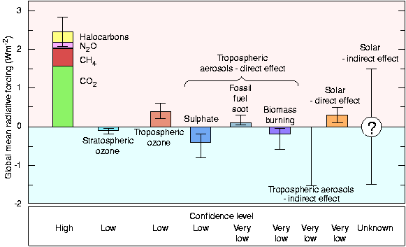
A small systematic rise or fall in the global temperature is caused by a net imbalance (“forcing”) in the Earth’s energy radiation budget. The radiative forcing caused by the increase in the CO2 fraction since 1750 is estimated to be 1.5 Wm−2 (Fig. 1) , compared with the global average incoming solar radiation1 of 342 Wm−2, i.e. an imbalance of only 0.4%. After including the effects of all greenhouse gases (+2.45 Wm−2), aerosols2 (-0.5 Wm−2) and their indirect influence on clouds (-0.75 Wm−2, but poorly known), the present net radiative forcing from mankind is estimated to be about 1.2 Wm−2.

The climate models upon which the predictions of greenhouse warming depend have gradually improved as new effects and better data have been incorporated. They now provide a reasonable match to the observed variation in global temperatures over the last century. However they remain subject to significant uncertainties, especially from feedback mechanisms and from the effects of anthropogenic aerosols. The latter contribute directly by scattering and absorption of radiation and also indirectly by influencing cloud formation. Nonetheless it is in this climate of scientific uncertainty that major political decisions on greenhouse gas emissions are presently being made (Earth Summit in Rio de Janeiro, 1992, and UN Climate Convention in Kyoto, 1997) that will have a profound effect on the economic development of both the developed and the developing countries.

The need for such political decisions to be based on sound scientific grounds is self evident, and a major world-wide research effort on climate change is underway. 1By convention, the incoming solar radiation of about 1366 Wm−2 is averaged over the total surface area of the Earth, i.e. divided by a factor four, to give a global average of 342 Wm−2.

2Aerosols are 0.001–1 µm diameter particles of liquid or solid suspended in the air . Atmospheric aerosols include dust, sea salt, soot (elemental carbon), organic compounds from biomass burning, sul- phates (especially H2SO4 and (NH4)2SO4) from SO2, and nitrates (especially HNO3) from NO and NO2.

Aerosol concentrations vary typically from ∼100 cm−3 in maritime air to ∼1000 cm−3 in unpolluted air over land masses, but there are large variations from these values. Figure 1: IPCC estimates of the global annual averaged radiative forcings due to changes in anthropogenic greenhouse gases and aerosols from 1850–1992 (first seven columns of the figure) . Positive forcings lead to a warming and negative forcings cause a cooling.

Natural changes due to the Sun are indicated by the final two columns; the first is the IPCC estimate of changes in solar output over the same period and the second concerns the present CLOUD proposal to study of the influence of galactic cosmic rays on cloud formation. Since the galactic cosmic ray flux is modulated by the solar wind, this would provide a mechanism for indirect solar radiative forcing.

Solar Variability

In order to determine the influence of mankind on climate change it is first necessary to understand the natural causes of variability. A natural effect that has been hard to understand physically is an apparent link between the weather and solar activity—the sunspot3 cycle.

The observation that warm weather seems to coincide with high sunspot counts and cool weather with low sunspot counts was made as long ago as two hundred years by the astronomer William Herschel who noticed that the price of wheat in England was lower when there were many sunspots, and higher when there were few. The best known example of this effect is known as the Maunder Minimum , the Little Ice Age between 1645 and 1715—which ironically almost exactly coincides with the reign of Louis XIV, 3Sunspots are areas of the Sun’s photosphere where strong local magnetic fields (typically 2500 Gauss, to be compared with the Earth’s field of about 0.3 Gauss) emerge vertically . They appear dark because their temperature is about half of the surrounding photosphere (3,000 K compared with 5,800 K).

They are generated by the differential rotation of the Sun with respect to latitude: one revolution takes 25 days at the equator and 28 days at mid-latitudes. This transforms the quiescent dipole field into a toroidal field and eventually creates “knots” of strong localised fields.

These Knots May Penetrate

the photosphere to form sunspots, which appear cooler due to modification of the normal convective motions of the plasma by the strong magnetic fields. The sunspots first appear at high latitudes and then gradually migrate towards the equator. They eventually disappear by magnetic recombination, leaving a quiescent dipole field once more (but of opposite polarity). The cycle from dipole to toroidal and back to dipole field is known as the solar (sunspot) cycle and takes about 11 years on average.

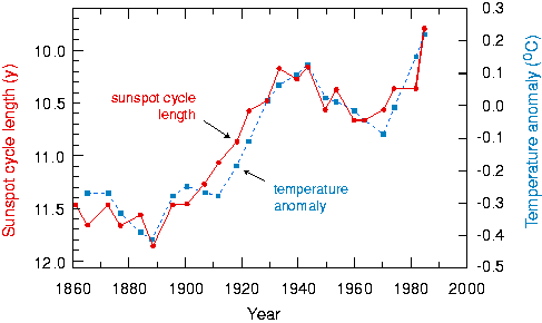
Figure 2: Variation during the period 1861–1989 of the sunspot cycle length (solid curve) and the temperature anomaly of the Northern Hemisphere (dashed curve) .

The

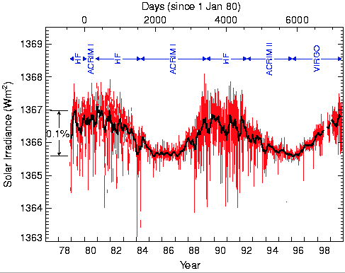
temperature data are from the IPCC . Figure 3: Satellite measurements of the variation of the Sun’s irradiance over two solar cycles . Sunspot maxima occurred around the beginning of 1981 and mid 1990, and sunspot minima occurred around the beginning of 1986 and 1996. The rapid fluctua- tions are due to sunspots rotating into the field of view. The solid line represents the smoothed data. The measurements are from active cavity irradiance monitors (ACRIM I and II) on the Solar Maximum Mission Satellites and from HF-type radiometers on the Nimbus 7 Earth Radiation Budget (ERB) and Earth Radiation Budget Satellite (ERBS) experiments.

le Roi Soleil, 1643–1715—during which time there was an almost complete absence of sunspots. During this period the River Thames in London regularly froze across and fairs complete with swings, sideshows and food stalls were a standard winter feature.

Since that time there have been numerous observations and non-observations of an apparent link between climate and the sunspot cycle –. One example of a positive observation was presented by Friis-Christensen and Lassen in 1991 (Fig. 2) . They used the sunspot cycle length as a measure of the Sun’s activity. The cycle length averages 11 years but has varied from 7 to 17 years, with shorter cycle lengths corresponding to a more magnetically-active Sun. A correlation was found between the sunspot cycle length and the change in land temperature of the Northern Hemisphere in the period between 1861 and 1989. The land temperature of the northern hemisphere was used in order to avoid the lag by several years of air temperatures over the oceans, due to their large heat capacity. The data shown in Fig. 2 cover the period during which greenhouse gas emissions are believed to be the major cause of the global warming of 0.6◦C. Of particular note is the dip between 1945 and 1970, which cannot be explained by the steadily rising greenhouse gas emissions but seems to coincide with a decrease in the Sun’s activity.

In the absence of sufficiently sensitive measurements, it was suspected that the Sun’s irradiance may be fluctuating over the solar cycle. However, the steadiness of the Sun’s irradiance over almost two sunspot cycles has recently been established by satellite mea- surements (Fig. 3) -. The solar irradiance is slightly higher at sunspot maximum; although sunspots are cooler and have reduced emission, this is more than compensated by an associated increase in nearby bright areas known as plages and faculae. The mean irradiance changes by about 0.1% from sunspot maximum to minimum which, if represen- tative over a longer time interval, is too small (0.3 Wm−2, globally-averaged) to account for the observed changes in the Earth’s temperature. However it is not completely neg- ligible, and current estimates—using the data shown in Fig. 3 together with the sunspot record—attribute a net direct radiative forcing over this century of about +0.3 Wm−2 due to changes in solar irradiance (indicated by the “solar - direct effect” in Fig. 1).

Osmic Rays And Cloud Variability

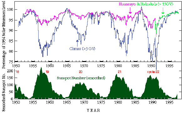
It is well known that the cosmic ray intensity on Earth is strongly influenced by the solar wind4 , whose strength varies with the sunspot cycle (Fig. 4 and Appendix D.2). The solar wind contains frozen-in irregular magnetic fields. Galactic cosmic rays that enter the solar system suffer many scatters from these irregularities and undergo a random walk. This has been theoretically shown to be equivalent to a heliocentric retarding electric potential, which varies over the course of the solar cycle. At times of low sunspot activity, the solar wind is weaker and the retarding potential at the Earth’s orbit is about 400 MV. At times of high sunspot activity, the retarding potential is about 1200 MV, thereby reducing the low-energy component of galactic cosmic radiation reaching Earth.

4The solar wind is a continuous outward flow of charged particles (mainly protons and electrons, with 5% helium nuclei) from the plasma of the Sun’s corona. Sources include streams from a honeycomb of magnetic fields in the solar atmosphere, and large and small mass ejections. The solar wind creates the huge heliosphere of the Sun that extends out 50–100 AU, well beyond the orbit of Neptune. At the Earth’s orbit the solar wind has a velocity of 350–800 km s−1 (β = 0.001–0.003) and an intensity of (0.5–5)×108 particles cm−2 s−1, carrying with it a magnetic field of about 5 × 10−5 Gauss.

Figure 4: Variation with time of sunspot number and cosmic ray flux, as measured by tron monitor stations at Climax, Colorado (3400 m elevation; 3 GeV/c primary charged particle cutoff), Huancayo, Peru (3400 m; 13 GeV/c cutoff) and Haleakala, Hawaii (3030 m; 13 GeV/c cutoff). The stronger modulation of the cosmic ray flux at higher latitudes (Climax) is due to the lower primary cutoffenergy. The neutrons are mostly produced by primary hadronic interactions in the first 1–2 λint of the atmosphere and therefore mea- sure the changes in cosmic ray intensity at altitudes above about 13 km. The primary cosmic radiation is about 80% protons, 15% He nuclei and 5% heavier nuclei. At sea level the most numerous charged particles are muons and their fluctuation is less pronounced— about 3% over a solar cycle —since they are produced from the high-energy component of cosmic radiation, which is less affected by the solar wind.

The cosmic rays are also deflected by the Earth’s geomagnetic field, which they must penetrate to reach the troposphere.5 This sets a minimum vertical momentum of primary charged particles at the geomagnetic equator of about 15 GeV/c, decreasing to below 0.1 GeV/c at the geomagnetic poles. (The actual cutoffat high latitudes is determined by the atmospheric material; for example a 1 GeV/c proton can penetrate only as far

As 15 Km Altitude.)

As a result the modulation of the cosmic ray intensity is more pronounced at higher geomagnetic latitudes (Figs. 4 and 52). Averaged over the globe, the variation of the cosmic ray flux is about 15% between solar maximum and minimum 5The troposphere is the lowest level of the atmosphere and the region where there is enough water vapour and vertical mixing for clouds to form under suitable conditions. The troposphere has a depth of about 18 km over the tropics, decreasing to about 8 km over the poles; it contains about 80% of the mass of the atmosphere. The troposphere is divided into the planetary boundary layer, extending from the Earth’s surface up to about 1 km, and the free troposphere, extending from 1 km to the boundary with the stratosphere (the tropopause). There is an overall adiabatic lapse rate of temperature in the troposphere of between 6◦C (moist air) and 9.7◦C (dry air) per km altitude, reaching a minimum of about -56◦C at the tropopause. The stratosphere extends up to about 50 km and has a temperature that slowly rises with altitude due to absorption of solar UV radiation. This leads to very little turbulence and vertical mixing and, in consequence, it contains relatively warm, dry air that is largely free of clouds.

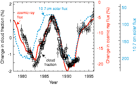
[22, 23]. It represents one of the largest measurable effects of sunspot activity near the Earth’s surface. But how could cosmic rays affect the Earth’s weather? The energy deposited by cosmic rays is only a few parts per billion compared with the incident solar energy, so a strong amplifying mechanism would be necessary. The breakthrough was made by Svensmark and Friis-Christensen in 1997 who discovered an unexpected correlation between global cloud cover and the incident cosmic ray intensity. The satellite data, which are shown in Fig. 5 (taken from the later ref. ), display a clear imprint of the solar cycle on global cloud cover.6 Over a sunspot cycle, the absolute variation of global cloud cover is about 3%, to be compared with an average total cloud cover of about 65%, i.e. a relative fraction of about 5%.

Figure 5: Absolute percentage variation of global cloud cover observed by satellites (data points; left hand scale) and relative percentage variation of cosmic ray flux (solid curve, normalised to May 1965; near-right hand scale) [1, 24]. Also shown is the solar 10.7 cm microwave flux (dashed curve, in units of 10−22 Wm−2Hz−1; far-right hand scale). The cloud data are restricted to oceans; Nimbus 7 (triangles) and DMSP (diamonds) data are for the southern hemisphere over oceans, and ISCCP-C2 (squares) data are for oceans with the tropics excluded. The error bars indicate representative statistical errors. The cosmic ray data are neutron measurements from Climax (Fig. 4). All data are smoothed using a 12-month running mean. A more recent analysis is shown in Figs. 6 and 7.

In addition to this observation of cloud variations over the timescale of order one solar cycle, other data sets have been analysed to investigate transient effects on clouds due to sudden changes in the cosmic ray flux. Forbush decreases of galactic cosmic rays occur due to solar disturbances on timescales of order days and therefore allow study of short- term cosmic-ray induced changes. Pudovkin and Veretenenko report observations of a short-term decrease of cloudiness that correlates with Forbush decreases, using a superposed epoch analysis on data obtained visually. Their observation is restricted to a narrow range of latitudes (60N–64N), and they suggest that cirrus clouds are responsible.

6The terms cloud cover, cloud frequency and cloud fraction are interchangeable. A similar analysis of the effects of Forbush decreases on rainfall has been carried out by the Forbush events recorded between 1956 and 1992. A 30% drop in rainfall (corresponding to a 3σ change from the mean) is observed on the initial day of the onset of the Forbush decrease.

A detailed mechanism modifying ice clouds has been proposed in a series of papers (notably Tinsley and Dean ), which suggests that significant changes in the latent heat released within supercooled clouds can occur as a result of aerosol electrification. The proposed mechanism is that charged aerosols are more effective than neutral aerosols as ice nuclei, which are generally rare in the atmosphere. The aerosol electrification is due to the ionisation created by cosmic rays. Rather than a comparison with cloudiness, Tins- ley’s superposed epoch analysis uses a dynamical parameter, the Vorticity Area Index (a measure of the regional scale motion), for which he finds a correlation with Forbush de- creases. The mechanism of latent heat release via electrical enhancement of ice nucleation can lead to substantial amplification of the ionisation energy deposited by cosmic rays in the atmosphere.

Other Solar-Induced Climate Variability

Other solar activity also follows the sunspot cycle, so in principle the cloud variations might be attributed to (a) a direct effect of cosmic rays on clouds, (b) a direct effect of other solar activity on clouds, or (c) an effect of solar activity on global weather that indirectly results in a change in cloud cover.

Although the other explanations mentioned here cannot be ruled out, Fig. 5 contains evidence favouring (a), the direct cosmic ray effect, which is to be investigated in the CLOUD experiment. The solar 10.7 cm microwave flux is a good proxy both for varia- tions in the sunspot count and for variations in the solar output of other electromagnetic radiation, namely visible light, X-rays and ultraviolet rays. In Fig. 5, the change in cloud fraction followed the cosmic rays closely but sometimes lagged as much as two years behind the change in the 10.7 cm flux. Delays in cosmic ray variations occur because dis- turbances in the solar wind, which scatter the cosmic rays, involve events (coronal mass ejections—CMEs, and co-rotating interaction regions) only loosely related to the sunspot count. Moreover the heliosphere is so large that disturbances can take up to about a year to reach its boundary, the heliopause. The delays show that the cloud variations correlate more closely with the cosmic rays than with the solar electromagnetic flux.

Could the solar wind have a direct effect on clouds, while coincidentally modulating the cosmic rays? This is unlikely because solar wind protons have very little energy (a few keV) and if they penetrate the Earth’s magnetosphere in the auroral zone, the outer atmosphere stops them at altitudes above 100 km. Shock waves associated with CME disturbances colliding with the slow solar wind can accelerate protons to 100 MeV or more, generating solar cosmic rays, but only rarely do they have sufficient energy to reach the tropopause at 8–18 km altitude.

The sign of the effect is a consideration in assessing possible solar mechanisms influ- encing the cloud fraction. While the cloud fraction correlates positively with the cosmic ray intensity, it correlates negatively with the solar electromagnetic radiation and with the strength of the solar wind. If enhancements in electromagnetic radiation or the solar wind were responsible for a direct effect on clouds, they would be in the counter-intuitive sense of reducing the cloud fraction.

As to whether changes in cloud fraction might be an indirect result of changes in global weather due to solar effects that coincide with the cosmic ray modulation, none of the other mechanisms on offer for a solar role in climate change suggests an effect on cloud

Fraction. Mechanisms Currently Discussed Include:

• Increases in visible light, causing warming at the Earth’s surface. • Increases in ultraviolet (UV), causing warming in the stratosphere .7 • Solar-induced turbulence in the Earth’s outer atmosphere that scatters gravity waves back to the lower stratosphere, again with warming effects .

All of these mechanisms seem likely to affect the geographical distribution of clouds, in particular by a poleward shift of the mid-latitude jet streams and depressions, during high solar activity. There is no obvious short-term link with cloud fraction.

Solar activity has many manifestations, and all of the means by which it may influence the Earth’s climate deserve further investigation. It is no part of our case to suggest that the link between cosmic rays and clouds is the only important solar-climatic mechanism.

For the reasons given in this section we nevertheless consider that the preferred interpre- tation of Figure 5 is the simplest, namely that cloud behaviour is directly influenced by cosmic rays. The opinion is reinforced by recent studies summarised in the next section.

Mproved Satellite Measurements Of Clouds

Currently the best continuous satellite observations of cloud properties are from the In- ternational Satellite Cloud Climate Project (ISCCP) D2 data, which covers the period from July 1983 to September 1994 [31, 32]. The D2 data are constructed by combining uniform analysis results from several satellites—up to five geostationary satellites and two polar orbiting satellites—to obtain complete global coverage every 3 hours. Cloud mea- surements are made at visible (λ ∼0.6 µm), near infra-red (3.7 µm) and infra-red (IR) wavelengths (10–12 µm). The IR measurements have the advantage that they provide continuous detection through day and night. As well as cloud frequency, the cloud-top temperatures and pressures are also determined.

The Temperatures And Pressures Are

obtained by assuming an opaque cloud, i.e. an emissivity ǫ = 1, and adjusting the cloud’s pressure level (effectively the cloud-top altitude) in the model until the reconstructed outgoing IR flux matches that observed. The clouds are classified into 3 altitude ranges according to the pressure at their top surface: low, >680 hPa (approximately <3.2 km); middle, 680–440 hPa (3.2–6.5 km); and high, <440 hPa (>6.5 km).

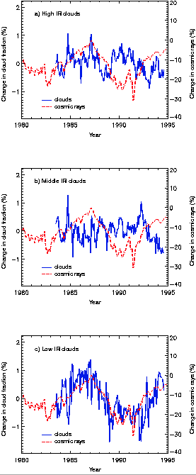
The cloud frequency for high, middle and low IR clouds is shown in Fig. 6 together with the cosmic ray variation over the same period . In contrast with the previous 7Only wavelengths above 300 nm penetrate to the troposphere and the Earth’s surface. These show a tiny peak-to-peak variation of less than 0.1% over the solar cycle.

However The Variation Is More

pronounced in the UV. Wavelengths below 300 nm, which account for only about 2% of the total solar irradiance, vary by about 5% (200–300 nm) to 50% (100–150 nm), or even more at shorter wavelengths . The UV radiation is absorbed by ozone in the upper stratosphere, which warms as a result. This has the potential to influence large-scale dynamics of the troposphere -, although vertical mixing between the stratosphere and troposphere is weak.

analyses [1, 24], these data are spatially and temporally unrestricted; they include clouds over the entire globe, during both day and night.

The Data Indicate The Presence Of

a significant correlation between cosmic ray intensity and the frequency of low clouds, below about 3.2 km, but none with clouds at higher altitudes. Since the cosmic ray and ionisation intensities—and their variations over the solar cycle—are largest above about 10 km altitude (Appendix D and Fig. 50), this would suggest mixing from the upper to lower troposphere may be involved. Indeed, vertical mixing is a prominent feature of tropospheric dynamics, where large-scale vertical transport of air, chemical species and ions can occur on timescales as short as a few hours via strong convective updrafts and the accompanying downdrafts.

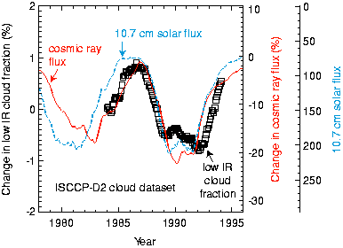
Figure 7 shows the low IR cloud fraction together with the variations of cosmic ray flux (solid line) and 10.7 cm solar irradiance over this period. The data are smoothed using a 12-month running mean to allow easy comparison with the earlier analysis shown in Fig. 5. The data confirm the presence of a solar cycle modulation of the cloud fraction, and continue to favour the cosmic ray interpretation.

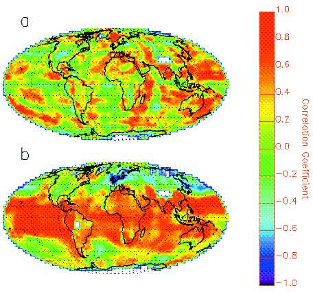
The global map of the low cloud frequency correlation is shown in Fig. 8a) . The fraction of the Earth’s surface with a correlation coefficient above 0.6 is 14.2%. Figure 8b) shows the correlation of low IR cloud-top temperature and cosmic ray flux. A strong and continuous band of high correlation (>0.6) extends throughout the tropics, covering 29.6% of the globe. This is a surprising result since the solar modulation of the cosmic ray intensity is a minimum near the geomagnetic equator, with a peak variation about 5% (Fig. 4). No significant correlations are observed between cosmic rays and the cloud-top temperatures of middle and high clouds (these data are not mapped here).

In summary, the ISCCP-D2 IR cloud data show a clear correlation of the cosmic ray intensity with low clouds, below about 3 km altitude (largely comprising stratocumulus and stratus cloud types), and no correlation with higher clouds. (As before, these data could alternatively be interpreted as a possible solar-cloud link via the UV irradiance.) The correlation appears in two distinct parameters: a) the cloud frequency (coverage), and b) the cloud-top temperature. The spatial distribution of the correlation across the globe is different in the two cases; the regions of high correlation of cloud frequency are widely scattered whereas the cloud-top temperature correlation is essentially continuous over the entire tropics. At present the reason for these different spatial distributions is not known, although we note that these are two separate cloud properties. Cloud frequency measures the presence or absence of a cloud, reflecting changes in the cloud lifetimes, cloud sizes, or cloud number. On the other hand, the inferred cloud-top temperature depends on its altitude and on the microphysical properties of existing clouds.

The signs of the two correlations are that more cosmic rays give more clouds and a higher cloud-top temperature. Under the assumption of opaque clouds, the cloud-top temperature effectively measures the altitude at the top of the cloud; a higher cloud- top temperature implies a lower cloud. However the observed properties of low maritime clouds suggest that they are not opaque . If the assumption of opaque clouds is relaxed, an alternative interpretation is that the cloud altitude does not change with increasing cosmic ray flux, but that the emissivity of the cloud increases. The latter could be caused by microphysical changes such as an increase in the droplet number concentration.

Figure 6: Monthly mean values for the global absolute variations of IR cloud coverage for a) high (<440 hPa), b) middle (440–680 hPa), and c) low (>680 hPa) clouds (solid lines) . Cosmic rays, measured by the Climax neutron monitor, are indicated by the dashed lines, normalised to May 1965. The mean global cloud fraction over this period for high, middle and low IR clouds is 13.5%, 19.9%, and 28.0% respectively. The cloud measurements are obtained from the ISCCP-D2 IR dataset [31, 32].

Figure 7: Variation over the period 1983-1994 of the low IR (10–12 µm) cloud fraction in the ISCCP-D2 dataset (from Fig. 6c) in comparison with the changes of cosmic ray flux (solid line) and 10.7 cm solar irradiance (dashed line). The cloud data have complete global coverage, day and night, and are smoothed using a 12-month running mean to allow easy comparison with Fig. 5.

Figure 8: Global maps of the correlation between cosmic ray intensity and a) low IR cloud fraction and b) low IR cloud-top temperature . The low IR cloud fractions are calculated as in Fig. 6c), while the low cloud-top temperatures are obtained from the ISCCP-D2 IR model. White pixels indicate regions with either no data or an incomplete monthly time series. The correlation coefficients are calculated from the 12-month running mean at each grid point. Fractions of the Earth with a correlation coefficient ≥0.6 are a) 14.2%, and b) 29.6%, respectively. The probability of obtaining a correlation coefficient ≥0.6 from a random signal is < 0.01% per pixel.

Effect of clouds on the Earth’s radiation energy budget The net radiative properties of a cloud are mainly dependent on its altitude and optical thickness. Optically-thin clouds at high and middle altitudes cause a net warming due to their relative transparency at short wavelengths but opacity in the IR region, whereas thick clouds produce a net cooling due to the dominance of the increased albedo of shortwave solar radiation. Since the data of Fig. 6 indicate that the solar modulation appears in the low clouds, the sign of the cosmic-climate effect is now known: increased cosmic rays are associated with increased low-clouds and therefore with a cooler climate.

Estimates from the Earth Radiation Budget Experiment (ERBE) indicate, overall, that clouds reflect more energy than they trap, leading to a net cooling of about 28 Wm−2 from the mean global cloud cover of 63% (Table 1) . The observed absolute variation in low cloud cover of about 2% over a solar cycle (Fig. 6c) corresponds to about 7% relative variation. From Table 1, this would imply a solar maximum-to-minimum change in the Earth’s radiation budget of about 1.2 Wm−2 (0.3% of the global average incoming solar radiation). This is a significant effect—comparable to the total estimated radiative forcing of 1.5 Wm−2 from the increase in CO2 concentration during the last century.

Table 1: Global annual mean forcing due to various types of clouds, from the Earth Radiation Budget Experiment (ERBE) . The sign is defined so that positive forcing increases the net radiation budget of the Earth and leads to a warming; negative forcing decreases the net radiation and causes a cooling.

History Of Cosmic Rays And Climate Change

If the periodic 11-year cycles of the sunspots and the associated cosmic ray flux were the end of the story, then it would be of limited concern since there would be no resultant long-term change in the Earth’s weather but simply another cyclic “seasonal” change (albeit with a period of 11 years and therefore heavily damped by the thermal mass of the oceans). However there is clear evidence of longer-term and unexplained changes both in the Sun’s and in the Earth’s magnetic behaviours and these, in turn, seem to have had long-term effects on the Earth’s climate.

Irect Measurement Of Cosmic Rays With Particle

detectors has been systematically carried out only during the last 50 years.

However

there exists another reliable record of cosmic ray fluxes on Earth, which stretches back for at least 200 millennia: the light radio-isotope record [22, 36, 23]. Light radio-isotopes interactions are induced mainly by low energy neutrons created in the secondary reactions of cosmic rays: protons, alphas and heavier particles. The two long-lived radioisotopes with the highest production rates are 14C (half life = (5730 ± 40) years, and global mean production rate ∼2.5 atoms cm−2s−1) and 10Be (half life = 1.5M years, global mean production rate ∼3.5×10−2 atoms cm−2s−1).

In the case of 14C atoms, they are rapidly oxidised to form 14CO2.

The Turnover

time of CO2 in the atmosphere is quite short—about 4 years—mostly by absorption in the oceans and assimilation in living plants. However, recirculation from the oceans has the result that changes in the 14C fraction on timescales less than a few decades are smoothed out. Plant material originally contains the prevailing atmospheric fraction of 14C and, subsequently, since the material is generally not recycled into the atmosphere, the fraction decreases with the characteristic half life of 14C.

In the case of 10Be, after production it rapidly attaches to aerosols (solid or liquid) and follows the motion of the surrounding air masses.

Since The Production Of 10Be

follows the intensity profile of the hadronic cosmic ray showers, about 2/3 is produced in the stratosphere and 1/3 in the troposphere, globally averaged. Due to the tropopause barrier, aerosols in the stratosphere take about 1–2 years to settle to the Earth’s surface, whereas the mean residence time in the troposphere is only days or weeks. The removal mechanism is rain and snow, and so seasonal variations of precipitation may distort any measurements on timescales less than a year or so. In summary, despite a factor 100 lower production rate than 14C, the advantages of 10Be are that it settles out relatively rapidly (<∼2 years) and it is not re-circulated into the atmosphere. It is therefore sensitive to changes in the cosmic ray flux on short time scales of only a few years. On the other hand, 14C has the advantages that it is not polar-centric and is independent of precipitation variability.

The change of cosmic ray intensity during the past century:

Analysis Of The

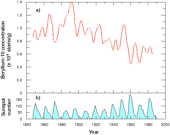
10Be concentration in a Greenland ice core (Fig. 9) reveals that the cosmic ray flux has been steadily decreasing over the course of the last century; it is weaker today at its maximum during the sunspot cycle than it was at its minimum around 1900. From refs. and , we estimate the global average reduction of cosmic ray intensity to be about 15% over the last century (with a range of 10–25%). This estimate is supported by direct measurements of cosmic rays over the last 40 years made by the Lebedev Physical The cause of this systematic decrease in the cosmic ray flux during the last century has been a marked strengthening of the solar wind and the interplanetary magnetic field it carries into the heliosphere. This is revealed by the geomagnetic index,8 for which there is a continuous record extending back to 1868, covering 12 sunspot cycles. Lockwood et al. have estimated the source magnetic flux, Fs, that leaves the corona and enters the heliosphere, from the level of geomagnetic activity seen at Earth in the index.

8The < aa > geomagnetic index is a sensitive measurement by two antipodal stations of short-term (3-hour interval) variations of the geomagnetic field at the Earth’s surface , which is affected by the interactions of the solar wind with the Earth’s magnetosphere.

Figure 9: a) Concentration of 10Be in a 300 m ice core from Greenland spanning the last 150 years . The data are smoothed by an approximately 10 year running mean and have been shifted earlier by 2 years to account for settling time. b) The sunspot cycle over the same period, which shows a negative correlation with the short-term (∼11 year) modulation of the 10Be concentration.

B)

Figure 10: a) The total solar open magnetic flux (coronal source flux) derived from interplanetary observations for 1964–1996 (thick solid line) and derived from the geomagnetic index for 1868–1996 (shaded curve) . b) The variation of the annual mean sunspot number.

Table 2: Decreases of the galactic cosmic ray intensity measured over the period 1957–

An ∼11-Year

smoothing of the data was applied to filter out the periodic solar cycle modulation.

%

This method to derive the coronal source flux has been successfully tested against near- Earth interplanetary space measurements made since 1963, during which time the coronal source flux of the Sun has been observed to rise a factor 1.4. In the period since 1901, Lockwood et al. calculate the increase to have been a factor 2.3 (Fig. 10). The reason for this dramatic increase in the Sun’s magnetic activity is a mystery.

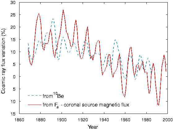
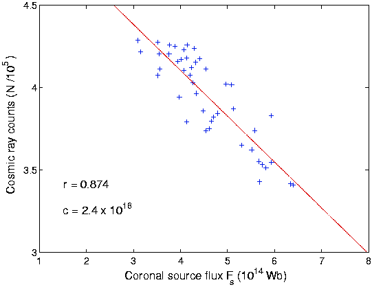
We have estimated the change in cosmic ray intensity over the last 140 years using these coronal source flux data. Scattering, gradient and curvature drifts caused by the he- liospheric magnetic field are the major contributor to the shielding of cosmic rays from the Earth and a very strong anti-correlation between cosmic ray fluxes with the heliospheric field near Earth was reported for the recent sunspot cycles 21 and 22 (Fig. 4). Thus an anti-correlation of the source flux Fs with cosmic ray fluxes is expected. This is seen in Fig. 11 which shows monthly mean counts, N, detected by the Climax neutron monitor in the interval 1953-1998 as a function of the annual estimates of Fs made by Lockwood et al.. The peak correlation (r = -0.874) is, essentially, 100% significant and is obtained with the cosmic ray fluxes lagged by one month. The line shows a linear regression fit to these data which can be used, along with the Fs data sequence, to extrapolate the cosmic ray flux variation back to 1868. The percent variation of the cosmic ray flux (relative to the average value for solar cycle 21) derived this way is shown by the solid line in Fig. 12. This extrapolation predicts a fall in the average cosmic ray fluxes of about 20% since 1900 for Climax (3 GeV cutoff), which implies about 15%, globally averaged, in agreement with the estimates given above. This change can be compared with the 10Be isotope record in ice sheets. The inferred cosmic ray variation is plotted as a dashed line in Fig. 12 and the long-term changes agrees well with the variation inferred from Fs.

If the cosmic-cloud link is real then this reduction of cosmic ray intensity implies a net positive radiative forcing equivalent to about one solar cycle, i.e.

+1.2 Wm−2

(Section 2.6) over the past century. In short, a systematic decrease in the cosmic ray flux of the magnitude indicated by the 10Be and coronal magnetic flux measurements could have caused a reduction in cloud cover and consequent warming of the Earth comparable to the observed rise of 0.6◦C in global temperatures last century, which is presently attributed predominantly to anthropogenic greenhouse gases.

Limate Change Over The Last Millennium

The observations of a correlation between the Sun’s activity, cosmic rays and the Earth’s climate can be extended to earlier times with either 10Be or 14C data. The latter agree Figure 11: The negative correlation of annual means cosmic ray counts, N, observed at Climax (cut-off3 GeV) and the coronal source flux, Fs (as estimated from geomagnetic observations). The peak correlation coefficient is r = −0.874, with the cosmic ray data lagged by one month. The probability of arriving at this result by chance is c = 2.4·10−16.

The solid line is the best linear regression fit. Figure 12: The estimated changes in the cosmic ray flux over the last 140 years. The solid line is the per cent variation (relative to the mean value for solar cycle 21) derived from the linear regression of cosmic ray fluxes with the coronal source flux. The dashed line is the variation derived from observations of the 10Be isotope concentration found in a Greenland ice core.

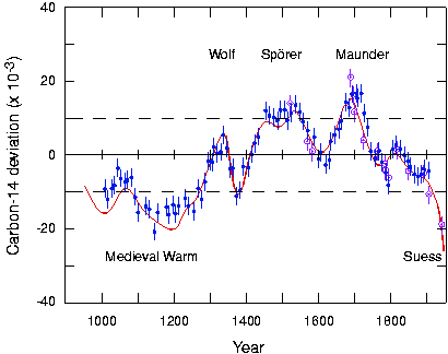
Figure 13: History of deviations in the relative atmospheric 14C concentration from tree- ring analyses for the last millennium . The data points (dots and open circles) are two independent high-precision measurements. The solid curve represents a combined fit to a large number of other measurements of medium precision. The dashed lines indicate 14C deviations of 10 parts per mil. The first four labelled periods correspond to recorded climatic anomalies. The sharp negative 14C deviation during the present century is the Suess effect, due to the burning of 14C-depleted fossil fuels.

well with 10Be data after accounting for a lag of ∼50 years in the 14C data due to the effects of re-circulation from the oceans . By analysing the 14C content in the rings of long-lived trees such the Californian bristlecone pine, a year-by-year record has been assembled of the cosmic ray flux on Earth over the past several thousand years. The data for the last 1000 years are shown in Fig. 13 .

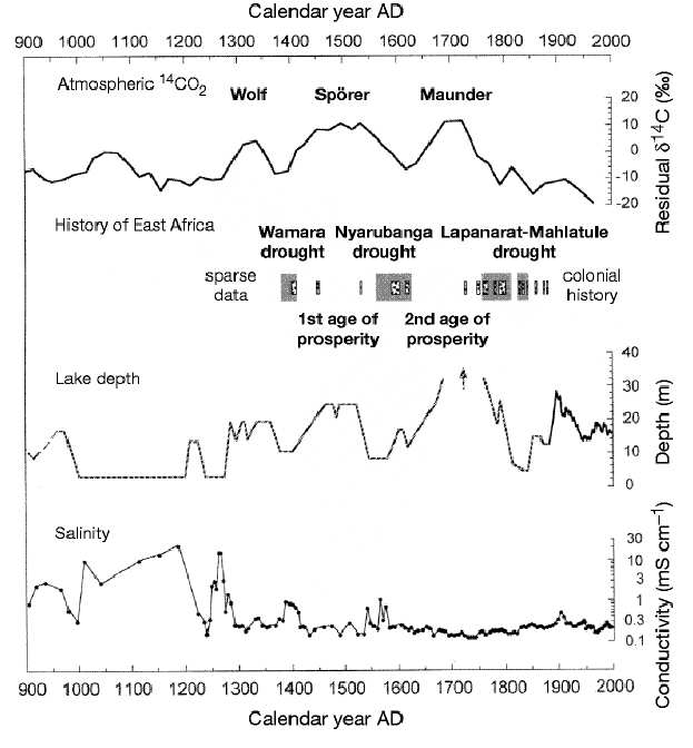
The periods where the 14C deviation approaches or exceeds 10 parts per mil correspond to recorded climatic anomalies: a) 1000–1270, the so-called Medieval Warm period, b) 1280–1350, the Wolf minimum, c) 1420–1540, the Sp¨orer minimum, and d) 1645–1715, the Maunder minimum. The warm period that lasted until about 1300 enabled the Vikings to colonise Greenland and wine making to flourish in England. It was followed by a period of about 500 years during which—save for a few short interruptions— the glaciers advanced and a cooler, harsher climate predominated.

The Maunder Minimum, when there was an almost complete absence of sunspots, cor- responded to a high cosmic ray flux on Earth and therefore, under the present hypothesis, to an increased cloudiness. This provides a consistent explanation for the exceptionally cold weather during this period. Indeed, in every case the lack (a) or excess (b–d) of 14C is consistent with the hypothesis of a higher cosmic ray flux leading to more clouds and cooler temperatures, and vice versa.

Evidence has recently been presented that this climate pattern extended into the equatorial regions, and is therefore likely to have been a global phenomenon. Figure 14 shows the correlation of the 14C record with the depth and salinity of a lake in equatorial East Africa over the last 1100 years . The reconstruction is based on three indepen- Figure 14: History of rainfall and drought in equatorial east Africa during the last 1100 years .

The central and lower figures show the reconstructed depth and salinity, respectively, of Crescent Island Crater lake (Kenya). The radiocarbon dating error for the lake data is ±50 y. The upper figure shows the atmospheric 14C deviation over the same period. Grey bars indicate evidence of drought-related political upheaval recorded in oral tradition, genealogically dated using a 27-yr dynastic generation. Dotted bars compile the evidence of severe drought periods from various archival records.

dent palaeolimnological proxies: sediment stratigraphy and species compositions of fossil diatoms and midges. These data not only confirm the presence of the major climatic anomalies associated with the Medieval Warm period and the Wolf, Sp¨orer and Maunder minima but also identify three extended drought periods between the minima: AD 1390– 1420, 1560–1625 and 1760–1840. The agreement with the 14C record is striking. The cultural history of the region, recorded in documents and oral tradition, coincides with the experimental data (see Fig. 14). In the present hypothesis, the periods of high cosmic ray flux would have corresponded to increased cloudiness. Under the assumption that in- creased cloudiness implies increased cloud lifetime, the rainfall would have decreased but at the same time the evaporative losses would have decreased. Which of these opposing effects would dominate depends on latitude and other regional effects.

These and earlier historical examples of climate anomalies provide strong evidence for solar variability and its coupling with the climate. One possible interpretation of the 14C data is that they provide a proxy for changes in the solar irradiance, and that this was the actual cause of the climate change. The alternative possibility is the mechanism addressed in this proposal, namely that the coupling is through the solar wind, cosmic rays and clouds. Regardless of the mechanism, however, there is little doubt that the Earth has experienced several extended warm and cold spells over the last 1000 years— and indeed at earlier times—with climate swings comparable to the recent warming but which could not be due to anthropogenic greenhouse gases. Whatever mechanism caused those earlier changes in the climate could perhaps be at work today.

In summary, there are two main conclusions to be drawn from the historical record of cosmic rays and climate change. Firstly, the pattern of systematic change in the global climate over recorded history seems to follow the observed changes of cosmic ray flux; and it is consistent with the explanation that a low cosmic ray flux corresponds to fewer clouds and a warmer climate, and vice versa.

Secondly, There Has Been A Systematic

decrease of the cosmic ray flux by about 15% over the course of the last century, caused by a doubling of the solar coronal source magnetic flux. The rise of about 0.6◦C in global temperatures over the last 100 years is consistent in magnitude and time dependence with the observed changes in cosmic ray flux—and thereby cloud cover—over the same period. If the cosmic-cloud link is confirmed then it provides a new mechanism for climate change that may significantly revise the estimated contribution to global warming from anthropogenic greenhouse gases. A clear and compelling case exists to investigate the causal link between cosmic rays and clouds.

Scientific Goals

The primary scientific goals of the CLOUD experiment are as follows: 1. To study the link between cosmic rays and the formation of large ions, aerosol par- ticles, cloud droplets, and ice crystals.

2. To understand the microphysical mechanisms connecting cosmic rays to changes in aerosol and cloud particle properties. 3. To simulate the effects of cosmic rays on aerosol and cloud properties under atmo- spheric conditions.

Concerning the last item, particular care will be taken to assess whether cosmic ray variations could have a significant effect on cloud properties within the natural variabil- ity of other factors. Where significant effects are found, we will attempt to provide the climate modelling community with simplified parameterisations of changes in key prop- erties of individual clouds. This will enable the influence of cosmic rays on clouds to be incorporated into GCMs (general circulation models) and an evaluation made of their contribution to the global radiative forcing over the last century (see Fig. 1).

(Deposition/ Freezing)

Figure 15: Paths that may connect cosmic rays to clouds and hence link solar and climate variability through the solar wind modulation. The processes are described in Section 3.2.

Paths Connecting Cosmic Rays And Clouds

Atmospheric clouds are highly complex and can be affected by a wide range of environ- mental parameters. At the simplest level, the development of a single small cumulus cloud is influenced by small changes in the temperature structure of the atmosphere, changes in humidity and surface heating rate. At a more complex level, the number of cloud droplets that form and their size distribution are affected by the composition and sizes of the aerosol particles upon which the water vapour condenses (Appendix A). There is also an enormous variety of cloud types, whose properties depend on the specific environmental conditions under which they form and develop.

This complexity makes it difficult to make a straightforward connection between cos- mic ray flux and cloud behaviour. Our approach in the CLOUD experiment is to: 1. Identify a number of key aerosol and cloud properties that might be affected by cosmic rays.

conditions relevant to the atmosphere. 3. Incorporate the experimental results in computer models of aerosol and cloud pro- cesses.

4. Simulate the behaviour of natural clouds with a variable cosmic ray rate to determine which cloud properties are sensitive to these variations. If cosmic rays can influence clouds, it is likely to be through their effects on aerosols or on ice nucleation. Aerosols are found throughout the atmosphere and constitute efficient cloud condensation nuclei (CCN) for activation of cloud droplets (Appendix A). The presence of a largely abundant supply of CCN ensures that the maximum water vapour supersaturations in the atmosphere rarely exceed values of about 1% since higher values are arrested by the removal of water vapour during droplet growth.

We have identified four distinct ways in which cosmic ray ionisation could, either directly or indirectly, affect clouds in the troposphere. The mechanisms are summarised in Fig. 15 and described individually in Sections 3.2.1–3.2.4 below. It is also possible that cosmic rays influence aerosol processes in the stratosphere, as discussed in Section 3.2.5.

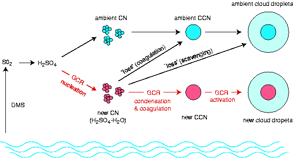
Enhanced aerosol nucleation and growth into cloud condensation nuclei Cosmic rays create ions in the troposphere, which may affect aerosol microphysical pro- cesses. Figure 16 shows a simplified set of atmospheric pathways that might connect variations of atmospheric ionisation with changes in the CCN abundance. The unbroken arrows indicate processes that are known to occur in the atmosphere. The arrows labelled ‘GCR’ are processes whose rate may be affected by ionisation. The most important pro- cesses affected are likely to be aerosol nucleation and aerosol particle growth either by condensation or by coagulation.9 Clouds that form in air containing high CCN concen- trations tend to have high droplet concentrations, which enhances the shortwave (solar) albedo. Increase in the CCN concentration also inhibits rainfall and therefore increases cloud lifetimes (cloud coverage). These effects—which are due to more, smaller droplets at a fixed liquid water content—are particularly significant in marine air, where the CCN concentrations are generally quite low.

The possible cosmic ray influence on CCN abundance indicated in Fig. 16 is similar to, but not the same as, the so-called aerosol indirect effect on clouds and climate. The aerosol indirect effect concerns changes in the supply of the aerosol material (such as SO2 in Fig. 16), which subsequently causes a change in the CCN abundance and hence cloud droplet concentrations. In the cosmic ray–aerosol–cloud indirect effect, which we propose to study, the cause of a change in CCN abundance would be changes in the rates of certain aerosol transformation processes.

It has been long speculated that atmospheric sulphate particles are formed by ion- induced nucleation (see, for example, refs. [41, 42] and references quoted therein). Also, 9Nucleation refers to the creation from vapours of a small (∼1 nm diameter), stable molecular cluster (aerosol) of a few tens or hundreds of molecules. Coagulation is the growth of an aerosol population by particles colliding and sticking together.

Figure 16: Possible influence of galactic cosmic rays (GCRs) on the nucleation of new condensation nuclei (CN) and on the growth into cloud condensation nuclei (CCN), ul- timately causing an increase in the concentration of cloud droplets. The arrows labelled ‘GCR’ are processes whose rate may be affected by cosmic rays. Dimethyl sulphide (DMS) from plankton is the major source of sulphur dioxide—the precursor of sulphuric acid—in remote marine environments.

processes such as ion-ion recombination have been proposed which lead to the production of stable molecular clusters in the lower stratosphere and in the troposphere [4, 5]. Since the nucleation rate of new aerosols from these processes is proportional to ion concentration, variations of the cosmic ray flux may translate into variations of aerosol particle concentrations and, ultimately, CCN concentrations. Recent experimental data suggest that ions may indeed be involved in gas-to-particle conversion. H˜orrak et al.

reported the spontaneous formation of bursts of intermediate size ions in urban air, which they suggest may be due to ion-induced nucleation. The Helsinki group has made similar observations of aerosol bursts in unpolluted marine air and in remote continental air .

Although the ion-induced nucleation phenomenon has been studied for more than 100 years, it remains poorly understood, both experimentally and theoretically. For example, the classical theory describes the charge effect on nucleation by an electrostatic interaction term between the ion and condensing molecules. However, this term does not explain the ion sign preference exhibited by many molecules (e.g. water molecules nucleate more easily on negative ions) which was experimentally found already by Wilson in 1899 . The sign preference has been attributed to surface orientation of dipolar molecules [48, 49], and a partial theoretical understanding has been proposed .

There is new evidence that increases in CCN concentration can indeed suppress rain- fall, and hence increase cloud lifetime. A recent study used NOAA satellite data to investigate clouds that formed downwind of industrial sites located in pristine areas.

The otherwise uniform cloud data from these regions was streaked with bright (highly reflective) plumes from the industrial sites. The droplets in these plumes were found to be more numerous than the nearby regions and of a smaller diameter—typically less than 10µm and therefore below the threshold size for them to coalesce efficiently and precipi- tate. In contrast the droplets outside the plumes measured more than 25 µm in diameter.

The high reflectivity of the plumes resulted from the high droplet number density at fixed liquid water content (Fig. 47). Independent analysis of data from the Tropical Rainfall Measuring Mission confirmed that these plumes did indeed produce less rain and there- fore had a longer lifetime than clouds in the nearby regions. These observations suggest that, if increases in cosmic ray flux could be translated into increases in CCN abundance, the observed increases in cloudiness (Fig. 7) could be due to decreases in precipitation efficiency.

Enhanced cloud condensation nucleus activation by charge attachment Aerosol activation is the rapid growth of an existing aerosol into a large (>∼1 µm) liquid droplet by condensation of water from a supersaturated vapour. If aerosol charging (in- duced by cosmic ionisation) could decrease the supersaturation needed for activation, this would lead to an increase in droplet number densities in clouds, with consequences for all cloud microphysical processes.

The possible effect of charges on aerosol activation has usually been ignored since the conventional electrostatic interaction term is expected to be appreciable only for very small aerosols of ∼1 nm diameter for small charges (see Appendix C). However, a recent study on heterogeneous nucleation of n-butanol vapour on charged and uncharged insoluble particles shows a surprisingly large charge effect. The charges have a clear effect on the nucleation process even when the seed particles are as large as 90 nm in diameter and the supersaturation is only 0.5%. For these experiments the classical theory predicts that the difference in the nucleating ability of charged and uncharged seed particles should vanish for particle diameters above 20 nm, corresponding to supersaturations of about 100%. If this result is correct, it indicates that charges may play a role in atmospheric cloud drop activation processes, at least when the CCN are partially insoluble (e.g. carbon) and carry multiple charges. Furthermore, the charges could influence the condensation of low vapour pressure trace gases on aerosol particles, and thereby affect the processes transforming CN into CCN.

Formation of condensable vapours and the effect on cloud condensation

Nuclei

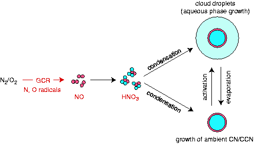
The ions and radicals, together with trace atmospheric gases, may promote the formation of condensable vapours or enhance the condensation of vapours already present, which can lead to the growth of existing aerosols (Appendix B). The condensation may occur on unactivated aerosols or on cloud droplets (aqueous phase growth), which would result in larger aerosol mass after evaporation of the water. Growth of aerosols can lead to a higher CCN number concentration, and to CCN that activate into droplets at lower supersatura- tions. The free radicals created by cosmic rays may also be able to influence atmospheric chemistry under certain conditions, especially if catalytic reactions are involved or where cosmic rays constitute a significant source of a chemical species [53, 54].

The most important radicals created by cosmic rays are N, O, and OH from the dissociation of the primary active constituents of air: N2, O2 and H2O. The estimated production rates are about 1–2 hydroxyl (OH) molecules per ion-pair and 1.5 nitric oxide (NO) molecules per ion-pair [55, 56, 57]. These rates imply mixing ratios of about 0.7 pptv NO are generated per day by cosmic rays directly in the upper troposphere.

After oxidation to nitric acid this may affect the growth of both CN and CCN (Fig. 17). Figure 17: Possible influence of galactic cosmic rays on the production of new condensable vapours and subsequent growth of existing CN and CCN.

Although the production of NO by cosmic rays is small on a global basis, it may be the dominant source in the upper troposphere of remote regions [55, 56]. Experimental evidence for the importance of particle ionising radiation for NO production is demon- strated by a clear nitrate signal in the Greenland ice core associated with solar proton events and the solar cycle [58, 59]. Calculations indicate that galactic cosmic rays may be responsible for about half of the NO in the polar stratosphere, and may be the dominant source during the polar winters when N2O oxidation is suppressed [54, 56].

Reation Of Ice Nuclei

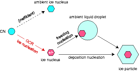
The presence of ice in clouds has an important influence on their radiative properties and it can also lead to precipitation. However the apparent lack of ice nuclei (IN) in the atmosphere is at present a mystery: there is about 1 IN per litre at 253 K (compared with about 106 aerosol particles per litre) whereas the observed concentrations of ice particles in clouds at these temperatures vary between 10 and 300 per litre. Two nucleation processes can lead to ice formation: a) direct sublimation of vapour to the solid phase (deposition nucleation) and b) freezing of a liquid droplet (freezing nucleation). It has been suggested that the ionisation produced by cosmic rays may be able to affect both deposition and freezing nucleation (Fig. 18).

The possible effect of charges on ice nucleation has been studied to some extent (see Pruppacher and Klett for a review), and effects have been seen in a number of experiments. Especially, the ice nucleating ability of various types of seed particles seems Figure 18: Possible influence of galactic cosmic rays on the creation of ice nuclei (IN) and ice particles at temperatures below 273 K.

to be influenced by ionisation. It is interesting to note that cloud chamber experiments in the regions where cosmic rays traversed the cloud chamber (Fig. 19)—although it was not possible to determine if the cosmic rays preceded or followed the droplet formation.

The presence of ions was observed to raise the threshold temperature for homogeneous ice nucleation by about 2 K. Enhancing heterogeneous ice nucleation by electrification has been proposed by several workers in the context of solar-terrestrial climate connections. It is supported by very little experimental work so far . If the electrofreezing effect is real, possible influences of cosmic rays on cirrus formation and on the properties of middle clouds are implied.

Electrofreezing could also affect glaciation (which triggers rain) in convective clouds. This may in some way be related to the correlation between cosmic rays and precipitation . The effect of cosmic rays on stratospheric clouds and ozone depletion The previous four processes have concerned aerosols and clouds in the troposphere. How- ever, cosmic ray intensities are even higher in the stratosphere, so it is conceivable that they also have an influence on aerosol processes in that part of the atmosphere .

Chemical reactions on stratospheric aerosols are a prerequisite for seasonal ozone deple- tion in both the Arctic and Antarctic stratosphere . These reactions convert relatively inert inorganic chlorine compounds into photochemically labile forms that can enter into ozone-destroying gas-phase catalytic cycles. The formation of polar stratospheric clouds in the low temperature polar stratosphere dramatically accelerates the rate of these reac- tions, leading to the formation of the ozone hole.

Significant advances have been made in our understanding of polar stratospheric cloud formation in the last 10–15 years [64, 65]. However, there remain important uncertainties that prevent a reliable prognosis of ozone depletion rates in a given winter or in future years. Chief among these uncertainties is what controls the phase (liquid or solid) of polar stratospheric cloud particles. At temperatures above the ice frost point the particles may Figure 19: Ice and liquid water droplets observed together in a cloud expansion chamber at 230 K. The two clusters correspond to regions of ionisation due to cosmic rays that crossed roughly along the direction of view. The ice droplets visibly scatter more light than the liquid droplets, and appear larger. In fact the large apparent size of the ice crystals is probably the result of light scattering in the emulsion film. The field of view in this image is about 17 mm across and about 10 mm in depth. The data were obtained be either liquid solutions of nitric acid, sulphuric acid and water or else solid hydrates of nitric acid. The formation of solid hydrates is important because it allows the selective growth of a small number of particles that subsequently become large enough to sediment out of the stratosphere. This process leads to denitrification of the polar stratosphere and often to strongly enhanced ozone loss (see ref. and and references therein).

Several mechanisms are recognised to be important for the formation of solid polar stratospheric clouds particles [64, 67]. However, persistent and optically very thin clouds, often seen over several thousand kilometer regions cannot be explained by any recognised mechanism. These tenuous hydrate clouds appear to be formed by a mechanism that operates on a very large scale with little spatial variability, thus excluding formation mechanisms involving localised cooling .

possibility that these solid particles form by crystallisation of the liquid aerosols by large scale cooling. An intriguing possibility—so far unexplored—is that these clouds form by deposition nucleation of nitric acid and water directly on cosmic ray-generated ions or ion clusters. However, to date, there have been no experiments that can confirm or dispute this possibility. An understanding of such particles appears to be critical to a complete understanding of denitrification and ozone loss.

Experimental Concept

The essential approach of CLOUD is to test the link between cosmic rays and cloud adjustable and collimated source of “cosmic rays”. The detector is based on an expansion cloud chamber that is designed to duplicate atmospheric conditions. This requires the capability of producing the very low water vapour supersaturations10—typically a few tenths of a percent—found in clouds, so that the precise cloud-forming properties of the air parcel under study can be measured.

The advantage of this approach is that all the experimental conditions can be pre- cisely controlled and measured. In particular, by comparing measurements at several beam intensities from zero up to high values, we can determine if there is a causal rela- tionship between ionising radiation and cloud formation. Such measurements are difficult to perform with cosmic rays in the atmosphere since the natural intensity variations are modest and they follow the slow 11-year solar cycle. Furthermore, the CLOUD experi- ment provides full control of the initial gas mixture and aerosol content and, in addition, complete physical and chemical analysis of the final products after beam exposure. This will greatly facilitate an understanding of the microphysics and chemistry of any observed atmospheric conditions and to ensure that the finite volume (walls) of the cloud chamber does not affect the measurements.

Surprisingly, cloud chamber data under atmospheric conditions in a particle beam have never been previously obtained. C.T.R. Wilson’s cloud chamber11 [70, 71] was extensively used for experimental particle physics in the first half of the 20th century, but was mostly operated under conditions far removed from those of the atmosphere. In order to grow droplets on the small ions produced by ionising radiation, Wilson cloud chambers were operated with water vapour supersaturations of 500–600%, to be compared with maximum values of about 1% in atmospheric clouds (see Appendices A and C).

However, It Is

interesting to note observations made in cloud chambers in the 1960’s of backgrounds due to “hypersensitive condensation nuclei” . These activated into droplets at very low water vapour supersaturations—of order 1%—and were attributed to trace amounts of NO2 vapour created by electrostatic discharges.

Nitial Experimental Programme

The initial CLOUD experimental programme and operating conditions are summarised in Table 3. It is important to note that our experimental search is quite broad since at 10Water vapour supersaturation, SS = S −1 = p/p0 −1, where S is the saturation ratio, p is the ambient partial pressure of water vapour and p0 is the saturated vapour pressure over a plane surface of water at this temperature. Supersaturation is frequently expressed as a percentage.

11Wilson had the inspiration for the cloud chamber while observing meteorological phenomena on the mountain of Ben Nevis in 1894. The phenomena were not particle tracks, however, but “coronas” around the Sun and glories, where the Sun glows around shadows in the mist. He developed the cloud chamber to the development of nuclear and particle physics for the next half century and earned him the 1927 Nobel Prize in Physics, Wilson remained fascinated by atmospheric phenomena throughout his life .

Indeed, he devoted a large part of his later research life to seeking a connection between cosmic rays and clouds. We are therefore glad to propose a Wilson cloud chamber for this experiment. Table 3: Initial CLOUD experimental programme and operating conditions.

Ppm

† Aerosol number concentration: ∼500 cm−3. § Supersaturation [%] relative to liquid water, during activation. ‡ Relative humidity [%] during beam exposure.

⋆Supersaturation [%] relative to ice. present there is no clear microphysical explanation of the possible cosmic-cloud link. We therefore expect to adapt our investigations according to our experimental observations and to the current experimental and theoretical developments at the time of taking data.

The initial experimental programme described here should therefore be considered as representative rather than definitive. Each experiment will in general be performed with two different carrier gases: a) pure Ar (inert carrier), b) pure artificial air (80% N2, 20% 02). The cloud-forming properties and other physical and chemical characteristics of the aerosols will be measured under beam/no-beam conditions using a range of equipment described in Section 4.

In the following subsections we outline some of the experiments required to explore the mechanisms described in Sections 3.2.1–3.2.5.

Aerosol Nucleation And Growth Experiments

These studies concern the formation of aerosols from the vapour phase, via ion-induced nucleation, and their subsequent growth by vapour condensation and coagulation. We will investigate the clustering of trace gas molecules onto ions.

The Trace Gas

molecules will either be formed by the ionising particle beam in pure artificial air or be introduced directly into the chamber. Such trace gas molecules include, in particular, H2O, H2SO4, HNO3, NH3 and certain volatile organic compounds.

These Trace Gases

will be measured by CIMS (Chemical Ionisation Mass Spectrometry), and the ions will be measured by ion mass spectrometers and ion mobility analysers. During activation measurements in the cloud chamber a fairly high supersaturation (large expansion) will be required, depending on the size and nature of the nucleated aerosols.

A major goal of these studies is to find out what fraction of the small ions created by ionising radiation become stable aerosol particles.

This Fraction F Will Increase With

decreasing temperature T and with increasing abundance of the clustering trace gas molecules. For example, in the case of H2SO4/H2O ion clusters, f is expected to in- crease with increasing relative humidity and relative acidity. However, for low H2SO4 concentrations a kinetic limitation becomes important which is related to the limited ion- ion recombination lifetime tIR. It is therefore important to work under well-controlled conditions with respect to the total ion concentrations ni and thereby tIR on the one hand and the sulphuric acid concentration [H2SO4] on the other. Both ni and [H2SO4], along with [H2O] and T, must be precisely known and adjustable.

The link proposed in section 3.2.1 between aerosols and clouds includes also a charge- enhanced growth of aerosols from small size (Aitken mode, 20–100 nm diameter) into the cloud-condensation nuclei (CCN) mode (>∼100 nm) where they can efficiently activate to form cloud droplets. We will start with a study of aerosols that are common in the atmosphere and known to be important in cloud formation such as NaCl, (NH4)2SO4 and H2SO4. Both “dry” and aqueous-phase growth will be studied. We will begin with well-known, simple systems to first confirm that the apparatus is well understood. This involves measurements with monodisperse NaCl or (NH4)2SO4 aerosols of diameter 10 nm, followed by 20 nm and then 40 nm. Then a second or third vapour component will be added and more complex systems studied.

Comparisons will be made with and without beam. Since diffusion of small ions is sig- nificant for beam exposures longer than about a minute (Section 5.4.3), the with/without beam measurements will be made in separate runs.

Because Of Their Relatively Small

mobility, the loss of aerosol particles to the walls of the cloud chamber is rather slow (Section 5.4.2) and, depending on the specific conditions, growth processes lasting 1–10 hours or more can be studied.

We will also investigate aqueous phase growth by taking measurements with several

↽Evaporation (Expansion ⇀

↽compression) cycles. The possibility that negative ions cause faster growth and condensation rates than positive ions will be investigated by selecting the ion charges with the field-cage of the cloud chamber (Section 5.3).

Loud Condensation Nuclei Activation Experiments

These studies concern the growth of aerosols into cloud droplets at relative humidities greater than 100%. Such aerosols, known as cloud condensation nuclei, have typical sizes in the atmosphere of 50-100 µm. Aerosols of a well defined size and with typical atmospheric composition (NaCl, (NH4)2SO4, H2SO4) can be produced with standard aerosol generation techniques (Section 4.4.3). Experiments will be performed to examine the activation of these aerosols into cloud droplets. The cooling of the cloud chamber by expansion will be sufficiently precise to be able to induce supersaturations with respect to water that are typical of the full range of values observed in natural clouds (Section 4.1).

Experiments with and without beam will enable the effect of aerosol charging on activation to be investigated. The charge distribution on the aerosols will be measured using a uniform electric field created by a field cage. In particular, we wish to know whether aerosol charging can reduce the critical supersaturation required to activate an aerosol particle into a water droplet. This can be investigated by counting the number of activated droplets as the supersaturation is gradually increased in separate experiments.

Ondensable Vapour Formation Experiments

These experiments will first quantify the poorly-known production rates of a) nitric oxide (NO) and b) hydroxyl radicals (OH) by cosmic radiation. The former will involve pure artificial air and the latter will involve argon and water vapour. Subsequently we will investigate the effects of these vapours on the nucleation and growth of aerosols.

Ce Nuclei Formation Experiments

These studies concern the formation of ice nuclei in supercooled vapours at low temper- atures. The expansion chamber will be used to create a supercooled cloud by expansion and growth of drops at temperatures below 260 K. The temperature of the drops can be controlled by the initial temperature of the chamber before expansion. The beam will be pulsed through the supercooled cloud and data recorded. The presence of an ice crystal in a cloud of drops is easily identified since an ice crystal scatters much more light than a water drop (Fig. 19) . The charge distribution on the ice nuclei will be measured using a uniform electric field created by the field cage. In addition to experiments with supercooled liquid droplets already present (freezing nucleation), we will also investigate ice nucleation without pre-existing droplets (deposition nucleation).

Stratospheric Cloud Formation Experiments

These experiments concern the deposition nucleation of nitric acid and water vapours onto ion clusters to form nitric acid hydrates. Particles composed of such hydrates are thought to be the principal component of the polar stratospheric clouds that initiate the destruction of ozone.

The temperature of the cloud chamber will be reduced to typical polar stratospheric values of between 190 and 200 K. Nitric acid and water vapour will be introduced into the chamber at partial pressures representative of the stratosphere (10−4 Pa for nitric acid vapour and 5 × 10−2 Pa for water vapour). At these pressures and temperatures the nitric acid hydrates become supersaturated and can condense as crystals provided a suitable nucleus is present. We seek to establish whether ion clusters can serve as these nuclei just as they can for the formation of sulphuric acid droplets in the stratosphere .

A background air mixture composed of water, nitric acid and sulphuric acid vapours will be used to represent the species most likely to contribute to initial ion cluster formation.

The Expansion Cloud Chamber Has Several Im-

portant advantages over other nucleation devices12 for the studies proposed here. In par- ticular, previous measurements with expansion chambers by our collaboration (Helsinki, Missouri-Rolla, and Vienna) have verified that the thermodynamic conditions after an expansion are precisely known and reproducible, provided that the initial conditions are well-known and the expansion ratio (pressure change) is well-measured. Moreover the expansion chamber can provide a large volume with uniform thermodynamic conditions where, for example, relatively slow processes can be measured. Expansion chambers may in fact be the only devices that can achieve the necessary thermodynamic stability and supersaturations (few × 0.1%) found in clouds and, in addition, cover the full range of supersaturations up to those required to activate small ions and nanometre-sized aerosols.

Size Of Cloud Chamber:

A large cloud chamber (∼50 cm diameter) achieves the longest time of known thermodynamic conditions in the fiducial volume13 of the chamber. The sensitive time14 ranges from about a second for expansions that produce high enough su- persaturations in water vapour to activate ions (a large difference in temperature between the walls and the gas) to several tens or even hundreds of seconds for the activation and growth of large aerosols (a small difference in temperature) (Section 5.2). The sensitive 12Besides the expansion cloud chamber, other experimental devices for studying nucleation include the thermal diffusion cloud chamber, cooled-wall expansion chamber, shock tubes and turbulent mixing chambers.

13The fiducial volume is the central region of the chamber where the thermodynamic and other condi- tions are well known, and where the measurements are made. 14The sensitive time following an expansion refers to the period during which no significant changes of thermodynamic conditions occur in the central part of the chamber caused by the heating influences of the walls.

time of an expansion chamber increases steeply with its size since it is proportional to the square of the ratio of the volume to wall area, which re-heats the gas following an adiabatic expansion. In addition a chamber size of about 50 cm ensures that diffusion losses of the aerosols to the walls are not significant for measurements lasting up to several hours with a single fill (see Section 5.4.2).

The Cloud Chamber Is Required To Operate At Water

vapour supersaturations (SS) from below zero (unsaturated) up to about 700%.

An

important requirement is to provide precise simulation of the conditions found in clouds, for which 0.1% <∼SS <∼1% (Appendix A).

This Supersaturation Range Corresponds

to a broad activation range of aerosols, namely radii from about 1 µm (at 0.1% SS) down to about 50 nm (at 1% SS). In order to probe the aerosol size distribution with sufficient resolution, the chamber needs to achieve a SS precision after expansion of about 0.1% in the range 0 < SS < 1%. Furthermore, the cloud chamber also needs to measure condensation nuclei down to small ion dimensions (0.2 nm), which requires large expansions producing supersaturations of up to 500%. The precision of the large SS values is, however, less demanding than for the small values.

Expansion Time:

The time duration of the expansion pulse needs to be short compared with the droplet growth time so that the start time is the same for all activated aerosols. This is especially important for experiments involving a broad size distribution of aerosols (to represent atmospheric aerosols), which activate over a relatively wide range of super- saturations. A rapid expansion ensures that the larger aerosols do not deplete the water vapour and prevent activation of the smaller aerosols. In practise the fastest required ex-

The Cloud Chamber Is Required To

operate over the full range of temperatures and pressures encountered by clouds in the troposphere and stratosphere, namely 173 K < T < 293 K and 0 < P < 101 kPa. The maximum pressure of the chamber is actually 150 kPa, in order to allow measurements to be made at 1 atm following a large expansion. It is important to note that the full range of pressure change can be addressed with our chamber design (Section 4.2.2). In a typical expansion chamber the pressure of the gas in the sensitive volume is used to drive the piston. For low pressures this becomes ineffective. In the cloud chamber proposed here, the piston is moved by a hydraulic system and thus a fast and precise expansion and re-compression can be achieved regardless of the pressure change in the chamber.

The Requirement Of A Precision Of 0.1% On

the supersaturation places demanding requirements on the temperature control of the cloud chamber. Taking a design value for the supersaturation error of one half this value, i.e. 0.05%, implies the need for a temperature stability ∆T = 0.01 K and a pressure stability ∆P/P = 1.3 · 10−4 or, equivalently, a volume stability ∆V/V = 0.9 · 10−4 (see Section 5.1, Eq. 6). Note that these are stability requirements; the absolute precisions of the temperature and pressure are less demanding.

Figure 20: Vertical section through the CLOUD detector. Figure 21: Horizontal section through the CLOUD detector. The CAMS detectors all lie in the same plane whereas the CCD cameras are displaced above and below the plane of the figure.

Overview

The CLOUD detector is shown in Figs. 20 and 21. The active volume is a cylinder of dimensions 50 cm (height) × 50 cm (diameter) and the fiducial volume is the central region of linear dimensions about 10–20 cm. The chamber is completely surrounded by a liquid bath which maintains precise temperature control. An outer vacuum enclosure, together with super insulation, maintains the thermal insulation of the inner detector.

The cloud chamber volume is equipped with an electrode structure (field cage) to provide a clearing field or the possibility to drift and measure charged aerosols. It also allows a method to select positive or negative charges for separate study.

Expansions are made by two techniques: a piston and a buffer expansion tank. The former is operated by a hydraulic system similar in design to the Big European Bubble Chamber (BEBC). The buffer expansion tank involves an external tank with a volume ten times larger than that of the cloud chamber. Expansions are effected by first reducing the pressure in the external tank to the desired value and then opening fast-acting valves connecting the external tank to the cloud chamber.

The optical readout of the cloud chamber comprises two systems: a) a constant angle Mie scattering (CAMS) detector and b) a stereo pair of CCD cameras. The two sys- tems are complementary but, nevertheless, have a broad region of overlap where they can provide mutual cross-checks. The CAMS system can measure very high droplet num- ber densities (∼10–107 cm−3) whereas the CCD cameras operate best in a lower range (∼0.1–105 cm−3). The CAMS system provides a high-resolution measurement of mean droplet radii vs. time, whereas the CCD cameras provide a measurement of droplet size in coarser time intervals, using pulse height information. Finally, the CAMS detector integrates over all illuminated droplets whereas the CCD cameras reconstruct the 3- dimensional spatial positions of individual droplets, and tracks their movements. This is important for identifying ice nuclei (Section 3.4.4) and for measuring droplet drift ve- locities (large droplet sizes).

The illumination system comprises: a) a laser for illumination of a narrow region for the CAMS detector (and, in parallel, for the CCD cameras) and b) a xenon flash tube for the CCD cameras, mounted at the top window (an auxiliary xenon flash system is also mounted close to the CCD cameras). A video camera is also mounted at the top window in order to provide a visual inspection of the chamber volume and piston surface.

The video camera and xenon illumination share the same window by means of a partially reflecting mirror (Fig. 20). The side windows are designed to allow simultaneous viewing of both the beam- and no-beam regions of the chamber. All windows are made of optical quality quartz. The use of quartz allows for the possibility of including UV irradiation to investigate reactions involving photochemical processes.

Cleaning of the chamber is very important to ensure reliable results.

The Upper

window is designed to be removable to allow cleaning access to the inside of the chamber and to minimise the transition time between different chamber fills. The chamber is also cleanable by vacuum baking. Vacuum evacuation is also an effective and rapid technique for removing a gas/aerosol mixture before refilling. Finally, large chamber expansions with a pure carrier gas can be used to confirm the cleanliness of the chamber before filling with a new mixture. Indeed, droplet activation and sedimentation is a proven technique Figure 22: Cloud chamber expansion systems: a) piston and b) external buffer tank.

to clean the cloud chamber to ultra low levels of contamination. The chamber is equipped with two sampling probes. These provide the possibility of extracting gas and aerosols from the fiducial region of the cloud chamber. They also provide the possibility for special measurements such as, for example, injection of a special gas into a limited region at the centre of the chamber. The probe tubes are straight and have a large diameter inner bore. All valves and pipes leading to and from the chamber are designed to provide efficient transmission of aerosols (large diameters and gentle curves).

A flow chamber (2m-length × 6cm-diameter) is integrated with the cloud chamber assembly and exposed to the same beam as the cloud chamber. It provides the source for external measurements of the physical and chemical properties of the trace gases, aerosols and ions with mass spectrometers, ion detectors, condensation particle counters (CPC) and differential mobility particle sizers (DMPS).

Expansion Techniques

The cloud chamber has a flexible choice of expansion techniques and expansion/ re- compression cycles. There are two expansion techniques (Fig. 22):

A) Piston:

Piston movement involves active control of the piston connecting rod by means of a hydraulic system similar in design to that used for the Big European Bubble Chamber (BEBC). An important advantage of piston expansions is that they minimise the gas turbulence, an effect that becomes more significant as the expansion ratio increases.

The piston also provides a flexible choice of precise expansion and re-compression cycles, with piston movements reproducible to very high precision—better than 5 µm.

The

range of piston movement is 5 µm to 200 mm i.e. volume expansion ratios of between 10−5 and 0.4. The very small expansions will provide supersaturations characteristic of those found in atmospheric clouds, while the largest expansions will activate aerosols of molecular/small-ion dimensions. The largest expansions also provide an effective method to clean trace condensation impurities from the cloud chamber by activation and then sedimentation.

B) External Buffer Tank:

This is a second method to produce small expansions. It involves a tank with a volume ∼10 times larger than the active volume of the cloud chamber, i.e. ∼1 m3. The tank is not cooled but has good thermal insulation to ensure that any temperature fluctuations are slow over the period of a particular measurement.

It is directly connected to the active gas volume via synchronised fast-acting valves at the top of the chamber. Expansions are effected by first achieving a pressure equilibrium with the valves open, then closing the valves, reducing the pressure in the buffer tank by the required (small) amount and finally re-opening the valves. The valves are left open during the sensitive time of the cloud chamber. The piston remains in a fixed location throughout.

An important advantage of this method is that it extends the sensitive time since it provides passive compensation for the pressure rise following an adiabatic expansion. The pressure rise occurs due to heating of the layer of gas near the walls and it causes a temperature rise throughout the volume by an adiabatic re-compression of the gas.

Operational Experience With Cloud Chambers

Some operational experience of our collaboration with cloud expansion chambers is sum-

Marised Below:

1. Reproducibility: The expansion ratio is determined from the initial and final pres- sures, since these quantities can be measured precisely—better than 10−4 absolute. Other quantities such as temperature change and supersaturation are calculated from the pressure change and the known initial conditions. In the 38 cm Missouri- Rolla chamber the pressure change is highly reproducible from pulse to pulse (a spread of about 2 · 10−4 for a large pressure change of 90 kPa).

2. Cycle time: The 25 cm Vienna chamber requires about 1 hr between expansions to allow time for thermodynamic equilibrium to be re-established. The 38 cm Rolla chamber requires about 5 min for equilibrium to be re-established following a deep expansion producing a temperature change ∆T = -40 K, during continual operation.

The cycle time is largely determined by how quickly the walls of the chamber can be brought back to the operational temperature following an expansion cycle. 3. Conditioning time: The 25 cm Vienna chamber requires 1–2 days conditioning prior to taking data.

4. Chamber cleaning: Based on 20 years experience with the operation of expansion cloud chambers at Missouri-Rolla, the following technique will clean a cloud cham- ber sufficiently for the demanding requirements of homogeneous nucleation mea-

Surements:

• The chamber is first fogged with liberal quantities of pure high quality water to dilute and remove water soluble components,. A fog nozzle sprays water drops over the chamber so that all surfaces are wetted and water runs down the walls. (In the CLOUD chamber the water will be injected through the sampling probe tubes.) After the application of about 4 litres, the water at the bottom of the chamber is removed with a tube suction device. After about 3 applications, a vacuum is applied to remove residual water.

• Acetone is then applied and is very effective at removing the last traces of water (particularly any water that has a surfactant preventing evaporation) as well as traces of any hydrocarbons etc., for which it is an excellent solvent.

The acetone is removed from the bottom of the chamber and the remaining (high vapour pressure) acetone is removed by vacuum evaporation. • Finally, the chamber is warmed under vacuum to remove the residual volatile contamination.

Piston And Hydraulic System

The piston expansion system comprises two main parts: the main piston and connecting rod, and the hydraulic system (Fig. 22a). The latter is based on the same design as was used to control the 2 m-diameter piston of BEBC .

The main piston head is made of a stainless steel envelope containing an inner stiffening structure. The piston has several grooves for holding spring-loaded PTFE seals which provide the gas seal with the walls of the cylinder. The upper surface of the piston is light-absorbing to reduce reflections from the top-window illumination (Section 4.3.2).

The outer region of the upper surface of the piston is shaped to provide a film of water for establishing 100% relative humidity in the active chamber volume. The inner structure of the piston is a sandwich assembly made of honeycomb and resin polymer plates reinforced with carbon fibre. This provides a good structural rigidity while maintaining a low mass.

A low mass is important since the required acceleration rates are large (up to 30 g) to achieve a fast expansion time for piston strokes up to the maximum of 200 mm. The main piston rod is made of stainless steel. The upper end of the rod is linked to the piston through a kernel which is dismountable for assembly and maintenance purposes.

The lower end of the rod is fitted with a hydraulic piston which is driven by the servo- mechanism. The servo-mechanism (Fig. 23) is made of several main components: a servovalve, a hydraulic pump, and high pressure and low pressure accumulators . There are three circuits containing liquid hydraulic oil: high pressure circuit (220 bar), low pressure circuit (20 bar), and the control circuit (running at a nominal pressure of 160 bar). All circuits

Control Hydraulic Circuit

Figure 23: Schematic diagram of the hydraulic system for piston expansions and re- compressions. are supplied by a hydraulic pump delivering an outlet pressure of 350 bar and a nominal flow rate of 20 l/min for a rotation speed of 1500 rpm. The power consumption is about 26 kW. The high pressure circuit feeds the high pressure accumulator (10 l capacity), which serves as an energy tank for the expansion. A low pressure accumulator (which is normally not present in these systems) is also included to avoid any shocks in the circuits or back effects at the end of the piston travel.

Each Of The Circuits Is Equipped With

pressure relief valves, with recuperation into a 100 l tank, and flow rate regulating valves. The control circuit drives the most critical component of the hydraulic system: the servovalve (Fig. 24). Depending on the electrical signal (±10 V) delivered by a computer, the spool slides inside the bushing of the control stage. The power stage spool is then moved, and the inlet/outlet connect the expansion chamber of the hydraulic piston with the high and low pressure accumulators. Any movement of the latter has then a direct effect on the main piston rod. The nominal control flow rate of the servovalve (control servovalve can reach 1500 l/min, which leads to an expansion time of about 150 ms for the maximum stroke of 200 mm. Shorter piston strokes are more rapid; for example, the expansion time is below 10 ms for a 5 mm expansion (which produces a supersaturation of about 6%). The limiting parameter is the ability of the main piston head to with- stand acceleration. The hydraulic system provides complete flexibility for the choice of expansion and re-compression cycles, which are determined by the analogue voltage pulse

Figure 24:

Principle of the servovalve for controlling the piston expansions and re- compressions. shape delivered by the control computer. The system also delivers an extremely precise (±5 µm) and reproducible (better than ±5 µm) movement of the piston.

The hydraulic piston (100 mm diameter) has no seal and its fit within the cylinder is of prime importance. A prototype of the main piston, hydraulic piston and servovalve system is required in order to validate the study and fix the parameters for the final installation, such as the pressure loss in the circuits and the leaks to be compensated.

The maximal allowable acceleration of the piston is another important issue that requires evaluation with the prototype.

Iquid Cooling System

The liquid cooling and temperature control system for CLOUD (Fig. 25) involves a closed circuit system, insulated throughout by vacuum. The liquid coolant flows through a jacket surrounding the cloud chamber and maintains the inner wall and piston at a precisely- controlled temperature. The gas inside the cloud chamber is allowed to reach thermal equilibrium with the walls before taking any measurements. A fluorocarbon liquid is used, such as FC87 (C5F12), which is liquid in the range 163 K–303 K at atmospheric pressure.

The fluorocarbon is transparent to visible and UV wavelengths down to about 180 nm. Consequently the liquid can circulate between the windows to obtain the optimum thermal jacket, without compromising the optical measurements or the option of UV irradiation Bosteels M.

N2

Figure 25: The liquid cooling and temperature control system. of the active volume. A coolant reservoir, circulation pump and heat exchanger are placed in a cold box.

The temperature of the circulating fluorocarbon liquid is adjustable in the range from 173 K–293 K. Temperatures are measured with Pt1000 platinum resistance thermome- ters which provide measurements stable to 0.001 K. The fluorocarbon is cooled by liq- uid nitrogen evaporating at a constant pressure, and re-heated by an electrical heater.

This allows fine temperature control and higher stability than can be obtained with a refrigerator unit. Our experience of similar liquid cooling systems for particle physics detectors shows that temperature stabilities of 0.1 K can be achieved for relatively large, non-insulated detectors involving internal heat sources and located in experimental halls without air-conditioning. In comparison, the CLOUD system is relatively compact, insu- lated throughout by a vacuum layer, and without any internal parasitic heat loads. This indicates that, with careful design, a temperature stability of 0.01 K can be achieved.

Field Cage

The walls of the cloud chamber are equipped with a field cage which provides an electric field inside the active volume. The functions of the electric field are as follows: • To clear ions and charged aerosols from the active volume.

• To allow measurements at below atmospheric ion concentrations. The typical ion concentration at the top of the troposphere is a few 1000 cm−3 (Section D.1); the Figure 26: Vertical section showing the flow chamber and beam counter system.

clearing field can lower the small ion concentration in the cloud chamber to near zero in about 2 s (Section 5.3). • To separate positive and negative ions and charged aerosols in order to measure their properties separately.

In addition, this will allow a technique for slowing charge neutralisation by +/- ion recombination. • To allow an approximate measurement of the aerosol size/charge distributions by measurement of the electrical mobility before activation. This is done by allowing the ions and charged aerosols to drift in a uniform field for a known time before the expansion pulse. The resulting droplets effectively freeze the final locations of the charged particles and allow their drift paths to be estimated and hence also their electrical mobilities. This provides a technique to check for consistency with the more precise mobility measurements provided by external detectors.

The field cage involves circular electrodes laid down on an 800 µm-thick ceramic insulating layer which lines the inside of the cloud chamber. The electrodes are continued across the chamber windows by means of thin, vacuum-deposited traces; these result in at the top of the cylinder completes the field cage. Except in the region of the windows, the electrodes are covered with a layer of black teflon, which is in contact with the gas in the active volume. The teflon has a small conductivity in order to avoid charge buildup and consequent field distortion. The cloud chamber walls and piston are grounded, and the field wire potentials are appropriately set relative to this ground, up to a maximum of 500 V. The performance of the field cage is summarised in Section 5.3.

Flow Chamber

A flow chamber of dimensions 2 m length × 6cm-diameter is integrated with the cloud chamber assembly (Fig. 26). It is filled with the same gas/aerosol mixture as the cloud chamber, and exposed to the same particle beam and, where required, to the same UV ir- radiation. Furthermore it is operated at the same temperature and pressure, but without the need for the same high precision on temperature and pressure stability. The exhaust gas from the flow chamber is analysed using condensation particle counters (CPC), dif- ferential mobility particle sizers (DMPS), mass spectrometers and ion mobility detectors (see Fig. 32 and Sections 4.4 and 4.5).

Onstant Angle Mie Scattering (Cams) Detector

The CAMS detection method allows simultaneous measurement of number concentra- tion and size of growing droplets. This method has been successfully applied in various experimental studies of nucleation and condensation processes [75, 76, 77]. A detailed description of theoretical and experimental aspects of the CAMS detection method can be found elsewhere [78, 79]. The general schematic layout of a CAMS system is show in Fig. 27 and the geometry for CLOUD is shown in Fig. 21. In the following the main features of CAMS are presented as they are relevant for the proposed research project.

Figure 27: Schematic diagram showing the experimental arrangement for the CAMS detection method. The CAMS detection method is based on light scattering. Growing spherical parti- cles are illuminated by a monochromatic, parallel light beam, e.g. a laser beam (Fig. 27).

The light flux Φtrans transmitted through the measuring chamber is monitored during the particle growth process by means of photodetector TD. Simultaneously, the light flux Φsca scattered at a selectable constant scattering angle Θ is monitored by means of photodetector SD. The observation cones of the detectors are defined by corresponding lens-pinhole arrangements L-PH. The actual sensitive volume VS inside the measuring chamber is determined by the intersection of laser beam and observation cone of detector SD for scattered light.

Our measurements from a typical CAMS experiment are shown in Fig. 28. Here si- multaneous growth of liquid drops in supersaturated vapour was observed. The vapour supersaturation was achieved by means of an adiabatic pressure jump in an initially sat- urated system. This pressure step is indicated by the upper curve in Fig. The middle curve in Fig. 28 shows (inverted) the transmitted light flux Φtrans as a function of time during the droplet growth process. The lowest curve shows the scattered light flux Φsca as a function of time. In the experiment considered a forward scattering angle Θ = 15◦ was chosen, the incident laser beam was linearly polarized perpendicular to the plane of observation.

As can be seen from Fig. 28, the experimental scattered light flux vs. time curve shows a series of maxima and minima. These extrema are connected to light diffraction and can be uniquely identified, as will be shown below. Thereby the particle size can be determined at each of the experimental extrema.

N The Absence Of Multiple Light Scattering The

experimental scattered light flux will be proportional to the number of particles inside the scattering volume. Accordingly, the droplet number concentration can be evaluated from the height of the experimental light scattering maxima independent of the determination of particle size.

The middle curve in Fig. 28 (inverted in the figure) shows that the transmitted light flux Φtrans decreases significantly during the droplet growth process.

Thus It Can Be

concluded that considerable light extinction can occur inside the measuring chamber, particularly at later stages of the particle growth process. This light extinction will be increasingly pronounced for increasing particle number concentrations. Obviously the ex- perimental scattered light flux will be reduced due to light extinction in the measuring chamber as well. Thereby the values of the particle number concentrations, as determined directly from the height of the experimental light scattering maxima, will generally be somewhat smaller than the actual concentrations. A correction for this light extinction effect would require the knowledge of the actual particle number concentration. Fortu- nately, the reduction of the scattered light flux due to light extinction can be taken into account in the following way. As seen from Fig. 28, the scattered light flux Φsca will suffer approximately the same light extinction as the transmitted light flux Φtrans, if the scat- tering volume VS is restricted to the central part of the measuring chamber. Thus the effect of light extinction on the scattered light flux can be compensated by normalising the scattered relative to the transmitted light flux. Accordingly, a linear relation between the normalised scattered light flux Φsca/Φtrans and the particle number concentration can be expected over a wide concentration range.

In order to achieve a unique quantitative interpretation of the light scattering curves as obtained from CAMS experiments, it is important to calculate the normalised scattered Figure 28: Result of a typical single CAMS experiments at Vienna for a forward scattering angle Θ = 15◦. The uppermost curve shows the pressure step in the expansion cloud chamber. The middle curve shows the (inverted) transmitted light flux, and the lowest curve shows the scattered light flux.

light flux Φsca/Φtrans as a function of droplet size for various constant scattering angles. The theory of light scattering by spherical particles has been derived by Mie and Debye ; a recent treatise by Bohren and Huffmann includes efficient numerical methods for evaluation of the relevant light scattering functions. Fig. 29 shows a comparison of experimental scattered light flux vs. time curves with theoretical scattered light flux vs. size curves for forward scattering angle Θ = 15◦. Satisfactory agreement between experimental and theoretical data can be observed allowing to establish a one-to-one correspondence of experimental and theoretical light scattering extrema.

The morphology of the light scattering curves depends on the size distribution of the growing droplets. As can be seen from Fig. 30, the resonant ripple structure of the light scattering curves tends to disappear with increasing width of the drop size distribution.

Thus CAMS measurements require sufficiently narrow drop size distributions to identify unambiguously a single peak in isolation. However it can be seen that the first scattering maximum at the forward scattering angle Θ = 15◦is not very sensitive to changes of the width of the drop size distribution.

When a unique correspondence between experimental and theoretical light scatter- ing extrema is established, the particle sizes at specific times during the growth process can be obtained from the positions of the extrema of the experimental normalised light scattering curves relative to the time axis. Independently, the droplet number concen- trations at specific times during the growth process can be determined from the heights of the maxima of the experimental normalised light scattering curve by comparison to the corresponding theoretical curve. In this connection it is important to note that, as mentioned above, the normalised scattered light flux Φsca/Φtrans is linearly related to the droplet number concentration. Determination of the droplet number concentration can

Tribution On Scattered Light Flux For For-

ward scattering angle Θ = 15◦.

Curves Are Labelled According To The Rel-

ative spread, σ, of the droplet radii. thus be performed by measurement of the ratio Φsca/Φtrans of scattered and transmitted light flux. To this end it is necessary to perform a mutual calibration of the detectors TD and SD for transmitted and scattered light fluxes, respectively. This calibration can be avoided by quantitatively considering the light extinction inside the measuring chamber.

From measurements of the light extinction at certain droplet sizes the droplet number concentration can be determined independently. The choice of appropriate scattering angles depends on the actual measurements to be performed.

For determination of particle concentrations it is advantageous to use comparatively small forward scattering angles, because the corresponding light scattering curves exhibit a rather simple structure with few broad maxima, which can easily be identified even for comparatively broad droplet size distributions. Furthermore, compar- atively high scattered light fluxes occur, allowing accurate measurements of the heights of the observed light scattering maxima. For measurements of drop growth rates, however, somewhat larger scattering angles are advantageous, because the corresponding light scat- tering curves show a somewhat more complex structure, providing detailed information on drop growth.

In summary the CAMS detection method is applicable to the observation of growing spherical particles (droplets) with known refractive index. The droplet size distribution needs to be sufficiently narrow so that distinct extrema can be observed in the experi- mental light scattering curves. Measurements over a comparatively wide range of droplet number concentrations can be performed. The lower limit of the concentration measur- ing range depends on the actual sensitive volume VS as determined by the incident laser beam and the observation cone of the detector SD for scattered light. In order to allow a unique evaluation of the experimental scattered light curves, generally more than about 5 particles must be simultaneously present inside the sensitive volume during particle growth. The upper limit of the particle concentration range will depend primarily on the amount of multiple scattering inside the measuring chamber . As shown recently , CAMS measurements show a linear concentration response over a range of concentrations up to as much as several 107 particles per cm3. Finally it should be noted that the CAMS detection method is a non-invasive method for absolute measurement of drop size and number concentration. No empirical calibration referring to external reference standards is required.

Cameras And Readout:

built a very fast, twin channel CCD imaging system for the August 1999 total solar eclipse, which is available for CLOUD. The SECIS (Solar Eclipse Coronal Imaging System) was successfully used to obtain in excess of 12,000 images during totality (i.e. in a period of less than 3 minutes) from a site close to the Black Sea in Bulgaria.

In essence, SECIS is an extremely fast, high-resolution imaging system. It is a con- siderable advance over previous systems in both frame rate and photometric accuracy. To meet the requirements of the solar eclipse observation, consecutive large area images needed to be stored at a very fast rate that was not until recently possible in any existing system but now is technically feasible using new developments in CCD cameras and mem- ory storage units. Currently, SECIS uses two small-area CCDs to obtain fast images and large on-line processing arrays to handle the image data. The computer system, interfaces and camera power supplies fit in a medium-sized, portable PC enclosure. Extra cooling is built into the enclosure to allow operation in hotter environments than normal. An uninterruptible power supply provides power for the whole system. Each frame of data is time-tagged for subsequent individual access from the PC.

The solar eclipse experiment required the capability of storing a large number (several thousand) consecutive frames of data without interruption. The two CCD cameras used are state-of-the-art digital cameras. Each has a 512×512 format with 15×15 µm2 pixels.

The data is digitised to 12 bits and clocked out at a frame rate of 55 Hz (which is well above the 10 Hz rate required for CLOUD). These images are “grabbed” by a specially- adapted PC, with dual Pentium processors. The PC has two PCI cards which provide the two camera interfaces; the cards are linked to ensure that there is no variation in timing between the two cameras. Exposure time and frequency are derived from programmable crystal-based oscillators. The operating system is Microsoft Windows NT Workstation.

The computer system captures two synchronised video streams from the two CCD cam- eras. It then reconstitutes the video images and stores them on a computer network for detailed off-line analysis. The data is buffered and sent to the computer via differential parallel cables. These also carry camera control signals generated by the computer to start and stop the light collection on the CCDs and to trigger the data transfer. The exposure time and frequency can therefore be selected by the operator.

The video data is packed by the PCI cards and temporarily stored in two buffer sets in main memory. As the buffers become full, the data is transferred to four SCSI disk drives, each 9 Gb in size. This is sufficient for about 36 min continuous operation at the full rate of 1 Gbyte/min (50 Hz). Each image is divided into 4 and each quarter image is stored on a separate hard drive. For data analysis, the reverse process takes the quarter images from each hard drive in the correct sequence and rebuilds the original full frame. These frames are then written out to the network disk as FITS images for compatibility with many different software packages. During normal operations, the workload is shared by the two processors. Two small live images can be displayed together with the buffer-filling status to allow the computer operator to monitor the performance of the system.

This system currently exists and is available for the CLOUD experiment. However, we are planning to upgrade the cameras to use newer CCD chips with a smaller pixel size and more pixels per chip.

Optics For The Cloud Chamber:

For the performance figures presented in this section, we will assume that each CCD camera has an upgraded chip of 1024 (h)×2048 (v) pixels, with a pixel size of 8 × 8 µm2 and an active area of 8.2 (h) × 16.2 (v) mm2. Since many CCD chips are already on the market with higher specifications,15 the figures presented here should be considered as conservative.

The CCD cameras are arranged in a stereo pair as indicated in Fig. 31. The optics are adjustable between a wide field-of-view and a narrow one. The former can be used to simultaneously measure regions of the chamber exposed to beam and not exposed. This requires a wide illumination field, which is provided by a xenon flash lamps mounted at the top window. This produces dark-field-illumination, i.e bright droplet images on a dark background. The flashlamps provide 100 J/pulse at up to 10 Hz; the power source is a 100 µF capacitor-bank charged to 1500 V. Experience with the 38 cm Missouri-Rolla chamber has shown, for xenon flash illumination, the scattered light intensity from a droplet is directly proportional to its radius in the range 2–20 µm. (This was the limit of the measurement; the proportionality probably continues either side of this range.) This indicates that the pulse height information from the CCD will provide measurements of the radii of individual droplets.

An alternative illumination scheme is provided by xenon flashlamps along the viewing direction (“ringflash” in Fig. 31). UV-absorbing filters (λmin = 450 nm) are used to avoid photo-ionisation reactions inside the chamber.

To Obtain The Best Sensitivity At High

droplet number densities, only the shallow region corresponding to the depth-of-focus of the CCD cameras is illuminated (see Table 4). This is achieved by focusing light from the upper xenon lamp with a cylindrical lens and collimating the beam with slits. The narrow field-of-view optics is optimised for measurements recorded at the same time as the CAMS detector, where a small volume within the acceptance of the cameras is illuminated by a narrow laser beam.

Some representative choices of the optical parameters are indicated in Table 4. For all 15An example is the Kodak KAF-6303 which has 3072 × 2048 pixels, with a pixel size of 9 × 9 µm2 and an active area of 27.6 × 18.5 mm2.

Figure 31: CCD camera optics and xenon flash illumination for the wide field-of-view. Table 4: Optical parameters of the CCD camera system. The figures assume a CCD chip of 1024 (h) × 2048 (v) pixels, with a pixel size of 8 × 8 µm2 and an active area of 8.2 (h) × 16.2 (v) mm2.

× 105

§ Full width of diffraction spot, at wavelength λ = 500 nm. † Limited by pixel size, not image diffraction. ⋆Assuming a centre-to-centre droplet separation of two pixels.

‡ Assuming 10% pixel occupancy. For the wide field-of-view optics, we assume the xenon flashlamp is collimated to illuminate the depth-of-field region. For the narrow field-of-view optics we assume CAMS laser beam illumination, with 20 mm of beam path subtended by the observation cone.

lens apertures larger than F5.6, the 8 µm pixel determines the size of a droplet image; this is larger than the diffraction limit of lens and the physical droplet size, for diameters below 10 µm. The wide field-of-view has a transverse size of about 9.2 (h) × 18.4 (v) cm2 and a depth-of-focus of 11–26 mm. A large field-of-view limits the maximum droplet number density to values of about 103 cm−3, which is adequate for most studies. If necessary, slightly higher values can be achieved by restricting the illumination to a shallower depth- of-field. In contrast, a narrow field-of-view allows measurements up to much higher droplet number densities of about 105 cm−3.

Overview

A schematic of the gas and aerosol supply and analysis systems is shown in Fig. 32. The supply system involves four components: carrier gas, water vapour, aerosols and trace gases. The carrier gas is either pure artificial air (80% N2, 20% O2) or argon. Water vapour, aerosols and trace gases are mixed into this stream at the desired levels (see Table 3). The water vapour and aerosol systems are described in more detail below.

Figure 32: Schematic showing the elements of the gas and aerosol supply systems and the

Water Vapour System

The water vapour content in the chamber will be set by two techniques: a) a liquid or ice film on the top of the piston and b) vapour and carrier gas introduced from an external humidifier. For most experiments, the saturation ratio before expansion will be p/p0 = (100.00 ± 0.05)%, where p is the partial pressure of the water vapour and p0 is the saturated vapour pressure over a plane surface of water (or ice) at this temperature.

(The error of 0.05% corresponds to a temperature variation of 0.01 K.) The vapour will be provided by a liquid or ice film covering most of the top of the piston and maintained

Authors:

Peder EZ Larson 1, 2,* , Jenna ML Bernard1, James A Bankson 3, Nikolaj Bøgh 4, Robert A Bok1, Albert P. Chen 5, Charles H Cunningham 6,7, Jeremy Gordon1, Jan-Bernd Hövener 8, Christoffer Laustsen 4, Dirk Mayer 9,10, Mary A McLean11 12, Franz Schilling13, James Slater1, Jean-Luc Vanderheyden5, 14, Cornelius von Morze 15, Daniel B Vigneron1, 2, Duan Xu1, 2, and the HP 13C

94143, Usa.

Denmark. 5 GE Healthcare, Menlo Park, California, USA. 6 Physical Sciences, Sunnybrook Research Institute, Toronto, Ontario, Canada.

8 Section Biomedical Imaging, Molecular Imaging North Competence Center (MOIN CC), Medicine, Baltimore, MD, USA. Cambridge, United Kingdom.

14Jlvmi Consulting Llc, Dousman, Wi, Usa

#See Acknowledgements for a list of all HP 13C MRI Consensus Group Members This work was supported by the ISMRM Hyperpolarized Media MR Study Group, the ISMRM Hyperpolarization Methods & Equipment Study Group, and the Hyperpolarized MRI Technology Resource Center (NIH/NIBIB grant P41EB013598).

Abstract

MRI with hyperpolarized (HP) 13C agents, also known as HP 13C MRI, can measure processes such as localized metabolism that is altered in numerous cancers, liver, heart, kidney diseases, and more. It has been translated into human studies during the past 10 years, with recent rapid growth in studies largely based on increasing availability of hyperpolarized agent preparation methods suitable for use in humans. This paper aims to capture the current successful practices for HP MRI human studies with [1-13C]pyruvate - by far the most commonly used agent, which sits at a key metabolic junction in glycolysis. The paper is divided into four major topic areas: (1) HP 13C-pyruvate preparation, (2) MRI system setup and calibrations, (3) data acquisition and image reconstruction, and (4) data analysis and quantification. In each area, we identified the key components for a successful study, summarized both published studies and current practices, and discuss evidence gaps, strengths, and limitations. This paper is the output of the “HP 13C MRI Consensus Group” as well as the ISMRM Hyperpolarized Media MR and Hyperpolarized Methods & Equipment study groups. It further aims to provide a comprehensive reference for future consensus building as the field continues to advance human studies with this metabolic imaging modality.

Keywords: Hyperpolarized MRI, metabolic imaging, carbon-13, pyruvate, dissolution dynamic

Introduction

MRI with hyperpolarized 13C agents, also known as hyperpolarized (HP) 13C MRI, has shown great potential as a novel imaging modality, particularly for its ability to probe metabolic processes in real time. The first human studies with HP [1-13C]pyruvate were performed in 2011 in prostate cancer patients (1).

Since then, there have been over 60 papers published with imaging results of human subjects from 13 different sites, with applications including prostate cancer, brain tumors, breast cancer, kidney cancer, pancreatic cancer, metastatic disease, liver disease, ischemic heart disease, diabetes and cardiomyopathies. The vast majority of these studies used [1-13C]pyruvate (1–63), where [2-13C]pyruvate (64) and 13C-urea (56) have been demonstrated too.

As clinical HP 13C MRI advances, there is a growing need to build consensus for best practices, which are critical for comparing data across sites, performing multi-site trials,deploying methods to new sites, partnering with vendors, and potentially for obtaining broader regulatory approvals.

In March 2022, we initiated an effort to build consensus within the HP 13C MRI community with this opportunity in mind, and it was greeted with strong enthusiasm. The “HP 13C MRI Consensus Group”, containing over 55 members from 27 sites, identified the area of greatest need and opportunity for consensus building to be HP [1-13C]pyruvate human

●

Pyruvate is the most mature and widely used HP agent and has the most significant translational evidence emphasizing the potential clinical impact.

●

Clinical trials, particularly multi-site trials, have the strongest need for consensus methods to ensure that data can be combined across sites. This work is a Position Paper for which the goal is to describe current successful practices and study methods for HP [1-13C]pyruvate human studies along with justification to support those practices. This is divided into four major topic areas: (1) HP 13C-pyruvate preparation, (2) MRI system setup and calibrations, (3) data acquisition and image reconstruction, and (4) data analysis and quantification (Fig. 1). The current successful practices and study methods include a literature review of published peer-reviewed journal papers showing human HP [1-13C]pyruvate study data, up to September 2022 (1–63), as well as new unpublished information from surveys of HP 13C study sites. Based on this information, we also highlight the evidence gaps, strengths, and limitations of current practices which are summarized at the end of each section.

Figure 1: Illustration of the HP 13C MRI human study process, including the 4 major areas covered in this paper: Hyperpolarized 13C-pyruvate preparation, MRI system setup and calibration, Acquisition and Reconstruction, and Data Analysis and Quantification.

Figure 2: Anatomical targets of HP [1-13C]pyruvate MRI human studies published up to September 2022.

Hyperpolarized 13C-Pyruvate Preparation

This section covers the processes for creating the HP agent, 13C pyruvate, and will include many aspects and considerations that are needed to safely and effectively prepare doses for metabolic imaging studies in human subjects. These include material, personnel, equipment and facility, fluid path preparation, quality control, and release.

It is helpful to understand that the specifications of a dose of 13C pyruvate suitable for in vivo MR HP metabolic imaging were shaped in part by early preclinical studies performed by GE HealthCare summarized in Ref. (65). In short, the safety of the two novel drug components, 13C pyruvate and the electron paramagnetic agent (EPA) AH111501, were demonstrated in those studies. The more precise formulation of the dose suitable for human use was then determined from clinical studies (66) that included two Phase 1 clinical trials in young and elderly healthy volunteers without hyperpolarization of the 13C nuclei and another Phase 1/2a dose escalation and imaging feasibility study with HP 13C pyruvate in 31 prostate cancer patients at the With the exception of the first HP 13C imaging clinical trial, which utilized a prototype device in a cleanroom (1), all HP 13C studies performed in humans to date have utilized the SPINlab polarizer (manufactured by GE HealthCare). Consequently all doses of the HP 13C pyruvate delivered by SPINlab have been produced using the “SPINlab Pharmacy Kit” that serves as the container-closure system for the various drug components (13C pyruvic acid and EPA mixture, dissolution medium, and neutralization and dilution medium) during sample polarization, dissolution and quality control (QC) processes. Thus many aspects of the HP sample preparation considerations discussed below are related to the SPINlab instrument and the consumables designed to be used with it (67).

General Considerations

While more than 860 patients or healthy subjects having been injected with HP 13C pyruvate as of January 2022 without reports of any serious adverse events (68), HP 13C pyruvate injection remains an investigational MR contrast agent and can only be administered by those with Investigational New Drug (IND) exemption from the Food and Drug Administration (FDA) in the USA, a Clinical Trial Application (CTA) in Canada, approval from National Research Ethics Committee Services in the UK, or approval from the relevant local regulatory body. Thus, methods and processes involved to produce a dose should have patient safety as the first priority. Since utilizing dissolution dynamic nuclear polarization (dissolution-DNP) for human use is still a relatively new development, there are no existing published regulatory guidelines specifically for this method.

There are two major production styles that determine how various sites approach the agent preparation. In the US, the most common approach is to rely on a sterilizing filter (“Terminal Sterilization”) to ensure sterility of the final product, akin to PET tracer production, where a starting molecule with a radioisotope is processed using various other ingredients to make the final, desired and injectable contrast agent within a necessarily short amount of time (69). For these sites, sterilization of the components and accessories upstream of this filter are not required, although many of them were manufactured and tested following Good Manufacturing Practice (GMP) or Good Laboratory Practice (GLP) requirements. The filling process is usually performed under an ISO 5 laminar flow hood, but a clean room or an isolator is not required.

This approach is typically accompanied by testing the integrity of the sterilizing filter prior to release of the dose for injection. Typically, post release endotoxin and sterility tests are performed using an aliquot reserved from each released dose.

In the UK and EU, the most common approach is to more-closely follow sterile pharmaceutical compounding guidelines (70), where all components and ingredients are required to be sterile or manufactured under GMP guidelines and are assembled and filled within a clean room environment or an isolator system (“Sterile Preparation”). Typically a batch of Pharmacy Kits for HP 13C pyruvate injection are prepared together. The sterility of the final dose is also ensured by batch validation testing, in addition to the sterility of the ingredients and the sterile compounding process. The endotoxin and sterility testing are performed for the process validation but are not performed for each injected dose.

Some institutions fill and assemble the Pharmacy Kit required for a specific study on the same day or the day prior to polarization, dissolution, and patient administration, but others have also demonstrated the feasibility of preparing a batch of kits, keeping them in a -20ºC freezer and using them over a period of a few months.

Beyond the obvious requirements that the process and the facility has to ultimately produce a dose that is safe to inject into a human, regulatory authorities will also focus on the question “Are you in control of your processes?”. To be in control of your process requires an in-depth and broad understanding of all processes involved in pre, post, and during the production process.

Personnel

It is typical and may be required to have licensed personnel involved in the production process depending on local regulations.Typically a pharmacist, radiopharmacist or other similarly qualified person (QP), in charge of the facility where the Pharmacy Kit filling and preparation is taking place, is responsible for the overall process and the release of the injectable dose.

Qualified cleanroom technicians are often involved in the Pharmacy Kit filling under the supervision of the pharmacist or QP. As is required for pharmaceutical compounding or PET tracer production, training requirements and training records for all personnel need to be maintained and available for audit by the FDA or equivalent.

Equipment And Facility

The facility and all equipment need to have standard operating procedures (SOPs) that describe how equipment is used, maintained, and calibrated to comply with relevant legislation. Currently, almost all the filling of the Pharmacy Kit takes place within a compounding laminar flow hood or isolator (typically ISO 5). At some sites, the filling is conducted within a cleanroom, while at others, it is conducted in a dedicated non-cleanroom space, reflecting differences in cleanroom approach and specifications between regulators worldwide (71). Some equipment or facilities, such as the compounding hood or cleanroom, may require external certified laboratories for testing.

Material Handling

Material handling guidelines (69,70) require SOPs detailing a system to track all of the materials involved in the HP production process for a particular patient dose, similar to current good manufacturing practice (cGMP) requirements for material handling for drug compounding. This includes acceptance standards, storage conditions, amount used in the patient dose for each ingredient and materials used in the assembly of the fluid path and Pharmacy Kit. Currently some users choose to open and inspect and sometimes modify the Pharmacy Kits upon arrival, but some users keep them in the sealed packaging until they are required for dose preparation.

Pharmacy Kit Filling And Assembling

As required by an IND or its equivalent, the preparation of the doses of HP 13C agent are detailed in the Chemistry, Manufacturing, and Control (CMC) section of an applicable regulatory submission; an example of this has been made available (72). It describes the processes of filling the Pharmacy Kit with the different components that make up the final drug product, and of assembling the final kit for either storage or immediate use in the polarizer. Special attention should be given to the laser welding process in order to satisfy installation qualification (IQ) and operational qualification (OQ). Typically, the final developed process is validated by process qualification (PQ) runs, during which 3 or more Pharmacy Kits are filled and used and the final HP 13C products are tested for endotoxin and sterility and to confirm that they meet the dose specifications for injections (usually including pyruvate concentration, residual EPA concentration, pH, liquid state polarization level and dose temperature). The data from 3 consecutive PQ runs are submitted as part of the IND submission (or its equivalent), and are often also reviewed by the Institutional Review Board (IRB) where the studies are conducted.

Quality Control And Dose Release

The quality control (QC) and dose release can be separated into two aspects: one is the QC and release of the filled Pharmacy Kit, and second is the QC and release of the HP 13C agent for injection, after polarization and dissolution. For institutions filling a batch of kits and storing them to use over a period of time, typically the batch can be released based on initial validation, environmental monitoring data from the day of kit production, and if filters are used during preparation of any of the components, filter integrity testing. But in some cases one or more kits are used for validation before the batch of kits are released for future use. For institutions that fill only the kits required for specific studies shortly before the experiment, the filled kits often do not go through separate release tests before they are used.

The quality control of the HP 13C pyruvate solution post dissolution is primarily performed to ensure that the agent meets the dose specifications (Table 1) before it is administered to the subject. These specifications target both safety (pH, residual EPA, temperature) and efficacy (pyruvate concentration, polarization, volume). Typically, the pyruvate concentration, residual EPA concentration, pH, dose temperature, dose volume, and liquid state polarization are measured by the QC accessory associated with the SPINlab polarizer. Some users perform a secondary measurement for one of the parameters, such as pH, using a different instrument or pH paper. For sites that do not go through a separate release testing process for batch filled kits, the integrity of the sterilization assurance filter, a part of the Pharmacy Kit, is typically tested as a part of the dose release. It is also common for these users to preserve an aliquot of the final HP 13C pyruvate solution for post-release endotoxin and sterility testing. This testing cannot be completed fast enough to test an individual dose prior to injection, but this is why other processes such as PQ runs and validation testing are done to minimize the chance a subject could be injected with a contaminated dose.

The Final Dose Release And Injection

should be done under the supervision of a licensed professional, based on local regulations.

Some Key Challenges

Many of the challenges associated with HP 13C pyruvate preparation can be attributed to the conditions required for the dissolution-DNP method of high magnetic field (~3-7 T) and very low temperature (~1 K) during polarization, with pressurized and superheated water necessary for the rapid dissolution event. These extreme conditions are quite challenging for the design of the container-closure and fluid path system. In particular, the cryogenic temperature in the polarizer requires special attention to any moisture or ambient (moist) air introduced into that portion of the fluid path, which can form an ice block at ~1 K. This ice can lead to flow restriction during the dissolution event and reduce the strength of the laser welded bond between the cryovial and its cap. This can ultimately produce failures in the dissolution step, including variations in final pyruvate concentration and pH that may fail to meet QC release criteria as well as fluid path ruptures that provide no available dose and result in polarizer down-time.

The polarization of the HP 13C pyruvate sample decays quickly over the span of a few minutes after dissolution, and thus the process of dissolution, QC for release, and injection should be completed as fast as possible to preserve the high polarization level achieved. Any delays in the preparation process, such as transportation time or equipment malfunction, can significantly reduce the final polarization and result in lower quality imaging data.

Current Practices

A summary of data collected from all sites performing clinical trials with HP 13C-pyruvate is shown in Fig. 3 and Table 1, including the specification of the final dose and how the quality control and release of the final dose are performed. There is a split in the Production Style, described in the General Considerations section above, with 8/13 sites using Sterile Preparation versus 5/13 using Terminal Sterilization. While many of the dose specifications show notable differences in acceptable ranges, all of these variations listed in tables have been successfully and safely been used to perform HP 13C pyruvate studies in humans. Their differences depend on the institutions’ preferences, resources and their particular regulatory situation. There is high similarity in pyruvate ranges, temperature ranges, EPA limits, and volume limits. There is modest variability in pH ranges and large variability in the endotoxin test limit. There is a 3-fold difference in acceptable polarization levels, which are measured to ensure a futile dose is not injected since the polarization is directly proportional to SNR. This reflects the decision by several sites to believe that useful data can be still be obtained with suboptimal polarizations.

Figure 3: Hyperpolarized agent preparation methods reported by sites currently performing HP

In House

Table 1: HP 13C-pyruvate preparation parameters, methods, and dose specifications used for quality control testing and release as well as validation. These were obtained from a survey of all sites performing clinical trials with HP [1-13C]pyruvate. The parameters used for product release are noted in bold text, otherwise these parameters are measured for batch validation or other QC measurements. The endotoxin and sterility testing are performed during process validation of the batch and/or post-injection, and largely depends on the agent production approach.

Summary

The overall safety record of HP 13C-pyruvate has been very strong, and the SPINlab hyperpolarizer has proven to provide high polarizations at human sized doses while meeting numerous QC and release criteria. A weakness remains the failure modes of the SPINlab Phamacy Kits (e.g. ice blocks, path ruptures), which are placed under extreme requirements particularly during dissolution. The preparation process still requires a high degree of expertise.

Therefore, there is a significant need to improve the reliability, robustness, and ease of operation for generating HP 13C-pyruvate doses for human studies. Furthermore, there is a divide between manufacturing and sterile compounding style preparation as well as other site-specific practices, resulting in variations in SOPs and justification required to relevant regulatory bodies. There have also been no comparisons between these approaches. It is also unclear what release criteria and QC parameters are truly required to ensure patient safety.

However, all of the reported methods are acceptable and approved by the appropriate regulatory authorities, and have led to the rapid expansion of successful human studies in recent years.

Mri System Setup And Calibrations

This section covers the MRI system setup, including the imaging system, RF coils, phantoms, and prescan calibration methods.

Imaging System

The main prerequisite for a given MRI scanner to be capable of supporting studies with HP 13C is its “broadband” capability to transmit and receive radiofrequency (RF) signal at the frequency of 13C, which is around 4 times lower than 1H. This does not come as a default on clinical MR devices. The transmit power of the broadband amplifier should also be sufficient to support the intended flip angle and RF pulse shape with the employed transmission RF coil(s) for 13C. Most studies to date use relatively low flip angles (< 90 degrees) for HP 13C in order to preserve polarization for time-resolved imaging. The capability to receive 13C signal on multiple channels is also desirable to increase SNR, as discussed further in the “RF coils” section.

The choice of magnetic field strength is primarily dependent on the metabolites’ frequency separation due to chemical shift dispersion and 1H imaging. High field strengths do not enhance hyperpolarized 13C signal as they do for 1H because the signal strength in a HP experiment relies on manipulating the population of quantum energy states outside of the MRI scanner.

However, the injected HP 13C-pyruvate and its metabolic products have greater frequency separation at higher fields, and it may thus be easier to separate and quantify these resonances at higher fields. This comes at the cost of a reduction in the achievable T2* and often reduced T1. As the initial polarization is independent of the imaging field strength it has been proposed that the increased T2* at 1.5T can potentially be exploited to increase SNR by adapting the acquisition bandwidth or reduce off-resonance imaging effects in cases when the decay of the transverse magnetization is dominated by T2* (73). In practice, 3T has been used in all published human 13C-pyruvate studies surveyed (Supporting Table S1), and comprises the majority of scanners currently in use for human studies (Table 3). A field strength of 3T is well-suited for 1H MRI anatomical reference and correlative imaging.

Stronger and more rapidly slewing magnetic field gradients support more rapid spatial encoding, particularly for metabolite-specific single-shot imaging using echo-planar imaging (EPI) or spiral imaging (See “Acquisition and Reconstruction”). Although the spatial resolution acquired for HP 13C imaging is typically much coarser than for 1H MRI, the factor of ~4 in gyromagnetic ratio leads to the same reduction factor in performance of the gradient system, so 13C experiments are potentially more limited by gradient hardware performance. To date, all human studies have used the commercially-available integrated gradient systems provided in clinical MRI scanners.

Optimization of scanner design has understandably focused on minimization of artifacts in 1H MRI, where devices such as room lights, the gradient amplifiers, and the motors driving the patient bed are checked to ensure that they do not produce RF interference at the 1H frequency, but artifacts may arise at other frequencies. Eddy current compensation is also not always appropriately adjusted for nuclei at other frequencies (74). In order to optimize for 13C, many sites have performed checks on phantoms for RF interference, gradient artifacts, and eddy currents (74), including the use of post-hoc gradient impulse response function characterisation and correction, and some vendors have fixed these issues as well.

Rf Coils

For HP 13C imaging studies in humans, RF coils for both 1H and 13C nuclei are needed, with 1H MRI providing an anatomical reference for registration and optional additional multiparametric MRI readouts. At the Larmor frequency of 13C nuclei, the relative contributions from coil noise compared to sample noise increase compared to 1H (73,75), although sample noise still is likely the dominant contributor for human-sized coils at 32.1MHz - the resonance frequency of 13C nuclei at 3T.

The key requirement for human 13C-pyruvate RF coils are that the coil geometry and sensitive volume must cover the volume of interest in the subject. Table 2 and Figure 4 shows coil configurations that have been used and optimized for applications in different anatomic regions.

Volume resonators are most commonly used for transmit, as they surround the subject to

Provide B1 Transmit Across The Fov (B1

+). While 1H relies on a large birdcage (“body”) coil built into the scanner, 13C transmit coils must be placed inside the bore. This takes up valuable space within the magnet, and also has led to the use of designs with relatively inhomogeneous

B1

+. Many human studies have used Helmholz pair resonators for transmit, including the “clamshell coil”, which has a notably inhomogeneous B1

+ Profile But Has Been Used Because Of

relatively easy integration into the scanner bore. B1

+ Variation Results In Variations In The Flip

angles that control the use of the hyperpolarized magnetization and creates errors in common HP metrics (9,76). The exception are head coils, where birdcage designs with highly

Homogeneous B1

+ can be placed around the head while easily fitting inside the bore. As with 1H MRI, higher SNR can typically be achieved by smaller receive coil elements, such as surface coils or phased arrays, and the majority of 13C receive coils used have layouts similar to 1H phased arrays.

RF coil quality control is important to ensure proper functioning of the coils to provide consistent imaging quality, especially with limited natural abundance 13C signal in vivo. It typically involves 1) a physical integrity check of the coil cables and connectors and 2) phantom SNR tests to check the coil’s performance and to monitor it over time (see Phantoms below). An useful reference for RF coil quality control is outlined in the MRI accreditation program of the American College of Radiology (77) and can be adapted for 13C coils.

Notably, configurations for brain and prostate studies used dual-tuned 1H/13C coil designs, which greatly simplify workflow and registration of 1H and 13C images, as no switching of coils is needed.

(1)

Table 2: RF coil configurations reported for human HP [1-13C]pyruvate studies.

Tx = Transmit

coil, RX = receive coil. The commonly used “clamshell” TX coil is a Helmholz pair design. For 1H RF configurations, all used the Body coil for TX unless otherwise noted, and “repositioned” indicates the 13C coil was removed for 1H imaging. One representative reference is listed for each configuration. The RF coil configurations reported in the reviewed papers are shown in Supporting Table S1.

Figure 4: Examples of RF coil configurations used for human HP [1-13C]pyruvate brain studies. (A,B) 13C Clamshell TX (Helmholz pair) and 2× 4-channel paddle RX arrays. (C) 13C Birdcage volume TX and 32-channel RX array (RX array slides into TX coil). (D) 13C Birdcage volume TX and 24-channel RX array, combined with a 1H 8-channel RX array. Image reproduced with permission from Ref (16).

Phantoms

Since hyperpolarized magnetization is non-renewable, phantoms containing 13C nuclei are important to: 1) test the multi-nuclear capabilities of the imaging system, including all parts of the signal excitation and receive chain; 2) perform calibration measurements before a scan with hyperpolarized nuclei; and 3) perform necessary pre-scan adjustments (see “Prescan Calibration” section). The phantoms currently in use are listed in Table 3. Their composition must provide sufficient 13C signal, with additional considerations of conductivity, stability, chemical shift(s) present, potential for dynamic imaging, and cost. The phantom geometries are typically either compact, in order to be used alongside the subject during a HP scan, or large enough to mimic the inner volume of a RF coil for system testing.

One popular compact design contains enriched 13C-urea at high concentration, typically 8 M, which provides a single resonance, placed inside a small container ~1 mL. The most common recipe mixes 13C-urea in a 90% water/10% glycerol solution, with glycerol used to increase the urea solubility and doping with a Gd-based contrast agent to shorten T1 which increases the potential SNR per unit time. For example, when Dotarem is added at a 3:1000 volume ratio the 13C-urea T1 is around 500 ms and T2 is around 100 ms. However, when testing pulse sequences influenced by T1 and T2, doping should be used carefully. This phantom is suitable for frequency calibration, transmit gain calibration, sequence testing, and as a fiducial marker when placed next to a patient. However, enriched 13C-urea has a relatively high cost compared to natural abundance compounds.

For larger volumes (>100 ml), the phantoms most often used contain undiluted ethylene glycol, glycerol, or dimethyl silicone. These compounds have sufficiently high carbon concentrations to provide sufficient 13C signal even with the 1.1% natural abundance of 13C. These larger phantoms matching the inner volume of an RF coil are useful for coil testing, including transmit

+) And Receive (B1

-) coil profile mapping, as well as to mimic acquisitions using in vivo FOV requirements. In this case, size and conductivity should match the expected subject size in order to mimic coil loading and get a realistic estimation of B1+. Large-volume natural abundance urea phantoms have also been used by some sites, but suffer from higher conductivity compared to biological tissues. Typically, it is easier to increase the conductivity and hence coil loading of the non-conductive phantom by adding NaCl to match physiological loading (16,78).

Dynamic phantoms that aim to mimic metabolite kinetics have also been developed (79–81), and have the potential to more closely mimic the HP experiment, but so far these are not widely used.

Prescan Calibration

Prior to performing an MRI acquisition, the so-called prescan procedure is used to set the shim parameters to maximize B0 homogeneity over the field of view (FOV) or a specific region of interest (ROI), the scanner center frequency (CF), the RF transmit gain, and the receiver gain.

While this calibration procedure is usually automated for 1H, the lack of sufficient natural abundance 13C signal prevents use of automated methods. (Although natural abundance 13C lipid signal has been detected, there are so far no reports on using this signal for prescan.) Table 3 shows current practices across sites.

Maximizing B0 homogeneity is independent of the nucleus and is therefore performed prior to 13C imaging using the 1H water signal and existing shimming tools, such as by a standard automated process (“Auto Shimming”) or using high order shimming routines. Similarly, the 13C CF can be calculated from the 1H CF using a predetermined scaling factor that depends on the target chemical shift (82). Another common approach used is to have a small, high-concentration 13C phantom, e.g. 8M 13C-urea, integrated in the RF coil or placed next to the scan subject (1). The reference frequency can also be based on real-time measurements after the HP injection but prior to imaging (83). Both the CF and B0 shimming are critical when using spectrally-selective RF pulses, as inmetabolite-specific imaging methods, where the desired excitation bandwidths are typically very narrow and frequency offsets can lead to a failure mode that is only apparent after injection.

The calibration of the RF transmit power is typically performed on a small, high-concentration 13C phantom placed near the region of interest during the scan or on a large 13C phantom of similar size and coil loading as the subject, prior to the subject scan. Reference power is often done by sweeping the power in a pulse-acquire sequence (53,62), or the Bloch-Siegert method (52,84). When using a small phantom, the location of the phantom, B1

+ Inhomogeneity As Well

as any shielding effects, e.g., when the phantom is integrated into a coil (1), may degrade the accuracy. Other methods include real-time Bloch-Siegert method measurements after the HP injection (83), and using the stronger natural abundance 23Na signal that is close enough to the 13C resonance frequency to be detected by 13C coils (82).

The receiver gain is predetermined, either systematically based on independent phantom measurements and assuming the dose and polarization of the HP compound is known prior to injection, or based on past HP imaging studies.

Power [Kw]

Phantom(s) - during study Phantom(s) - before study 13C Frequency

8

13C-bicarbonate doped with dimethyl silicone, various

Power [Kw]

Phantom(s) - during study Phantom(s) - before study 13C Frequency

Maximum Values

Table 3: Summary of the imaging systems, phantoms, and prescan procedures used at sites currently performing HP 13C-pyruvate human studies. These were obtained from a survey of all sites performing clinical trials with HP [1-13C]pyruvate. *Previously performed studies with a Siemens 3T Tim Trio. The imaging systems, phantoms, and prescan procedures reported in the reviewed papers are shown in Supporting Table S1.

Summary

Commercially available 3T MRI systems are by far the most commonly used for human HP 13C-pyruvate studies, although a systematic investigation of the impact of B0 has only recently been investigated (73). The multi-nuclear RF transmit and receive chain has proven sufficient for current acquisition strategies, although many sites have observed artifacts due to RF interference, gradient interference, and residual eddy currents when operating at the 13C frequency. A variety of 13C RF coils, tailored for numerous anatomical targets, have been successfully demonstrated, with the main limitation that most transmit coils take up a lot of additional space inside the bore and provide relatively inhomogeneous B1

+ Profiles. The

phantoms used have converged into generally 2 categories - small phantoms containing 13C-enriched compounds that can be used during the study and human-sized phantoms containing compounds with high carbon concentrations but without 13C enrichment that are used to test and calibrate the coils. There are no standardized compositions or geometry, and dynamic phantoms that recapitulate in vivo kinetics would be desirable but are still an emerging area. Prescan calibration procedures were not well defined in most publications, so we surveyed individual sites to determine current practices. Calibration procedures for the B0 field (13C CF and shimming) for most sites take advantage of 1H signal and methods, while methods

For Calibration Of B1

+ is more variable across sites, likely a reflection of remaining challenges in how to perform this calibration. Standardization of both phantoms and calibration procedures would synergistically improve the robustness and reproducibility of HP 13C studies.

Acquisition And Reconstruction

Data acquisition strategies in human HP [1-13C]pyruvate MRI studies must account for multiple chemical shifts, efficiently utilize the non-renewable HP magnetization, and acquire data quickly relative to metabolism and relaxation decay processes. These studies require spectral encoding to separate metabolites, necessitating pulse sequences that efficiently encode up to 5D data (3 spatial + 1 spectral + 1 temporal dimension). RF pulses must efficiently sample without immediately saturating the non-renewable HP magnetization, and sequences must acquire data quickly and be robust to both experimental and physiologic variation (e.g. B1

+ Inhomogeneity,

variation in perfusion) to ensure reproducibility and minimize scan-to-scan variability. This section covers current successful practices for data acquisition in human [1-13C]pyruvate studies, and accompanying 1H imaging, from different anatomic regions, including scan parameters and image reconstruction.

Acquisition And Reconstruction Methods

The acquisition methods used in human [1-13C]pyruvate studies can be classified into 3 categories: 1) MR spectroscopy or MR spectroscopic imaging (“MRS/I”), 2) chemical shift encoding methods, and 3) metabolite-specific imaging (Fig. 5).

Mrs/I Methods Specifically

resolve a spectrum that can be analyzed to extract expected as well as unexpected resonances, making this approach very robust. It was used in many initial studies (1).

Chemical Shift

encoding methods, most commonly the Iterative Decomposition of water and fat with Echo Asymmetry and Least-squares estimation (IDEAL) method, use imaging sequences acquired with multiple TEs and rely on a model-based separation of expected chemical shifts (85).

Metabolite-specific imaging methods use specialized RF pulses that are spatially and spectrally selective to excite individual metabolites which are then typically imaged with fast k-space trajectories such as echo planar imaging (EPI) or spirals (86).

Their Application To Different

organ systems is described below. The image reconstruction methods used in human [1-13C]pyruvate studies have typically been conventional methods (e.g. FFT, non-uniform FFT, or equivalent). The incorporation of accelerated imaging and advanced reconstruction methods including parallel imaging (4,57,87) and compressed sensing (7) has also been applied in human studies for improved spatial resolution, temporal resolution and coverage, but have the potential for additional artifacts as well as SNR losses due to ill-conditioning of the reconstruction (e.g. g-factor).

The Majority Of

published studies do not use accelerated imaging indicating the resolution and coverage achievable without acceleration is currently adequate for successful data collection. Performing coil combination, even with fully sampled data has also been shown to have specific challenges for HP human images: using naive sum-of-squares methods suffer from high noise amplification in the relatively low SNR regime of HP [1-13C]pyruvate (compared to 1H), motivating several HP 13C-specific methods that include data-driven coil sensitivity estimation which have shown obvious improvements over sum-of-squares (11).

More recently denoising techniques have been applied as post-processing of human HP data(41,42,44). The techniques applied are based on spatial-temporal singular value decomposition for unsupervised estimation of signal and noise components. They have shown improvements in apparent SNR in the brain and liver, while care must be taken to choose parameters such as the rank threshold to avoid oversmoothing and overfitting to the estimated signal components.

Prostate Studies

Prostate cancer was the first human application of HP [1-13C]pyruvate (1), and data was acquired with MRS/I methods: 1D dynamic MRS, single-slice 2D dynamic echo-planar spectroscopic imaging (EPSI), and single time point 3D EPSI. Advances in imaging strategies led to the development and application of new acquisition schemes, including undersampled 3D EPSI with compressed-sensing (7), model-based chemical shift encoding methods that use a priori information (47,59), and metabolite-specific EPI (10), all of which can provide volumetric whole-organ coverage and dynamic acquisitions.

The pyruvate bolus arrival in the prostate can vary by ± 10 s between patients, necessitating dynamic imaging to reliably and consistently capture the pyruvate bolus (18). For this reason, all currently ongoing studies acquire dynamic data. While MRS/I, chemical shift encoding, and metabolite-specific imaging can all achieve dynamic imaging, chemical shift encoding and metabolite-specific imaging provide greater dynamic and volumetric coverage (85). For scan prescriptions, the FOV is designed to provide full prostate coverage and typically to match the orientation of the anatomic imaging used for registration. Flip angles used in current studies are constant through time, as quantification with a variable-through-time flip scheme is highly sensitive to bolus timing (8) and errors in the RF transmit (B1 +) field (76).

Heart Studies

Data acquisition methods for 13C imaging in the heart must be designed to meet the demands of significant cardiac motion and blood flow. To cope with the periodic cardiac motion, most human heart studies to date used gating to the diastolic window, the longest cardiac cycle interval, which has reduced motion (2,22,28,30,35,36,38,45,52). The duration of the diastolic window limits the available data sampling time, making cardiac acquisitions the most time-constrained of the HP 13C MRI applications. The most common acquisition approach is metabolite-specific imaging with spiral k-space trajectories (2). Their single-shot imaging capability makes these methods particularly robust to motion effects. Furthermore, spiral k-space trajectories provide rapid k-space coverage and relatively benign flow and motion artifacts. The majority of studies have used 2D multi-slice acquisitions, but 3D encoding has also been used successfully (35).

Brain Studies

For HP 13C MRI of the human brain, the majority of studies have also used 2D (slice selective) acquisitions (10–12,14,16,28,33,40,41,44,51,53,60), with a trend toward volumetric coverage using 2D multi-slice metabolite-specific imaging. 3D metabolite-specific imaging of the whole brain, with phase encoding of the slice direction (34,57), has been shown to provide similar SNR efficiency (88) compared with multislice imaging. A number of studies have employed MRS/I (5,6,29,31–33,50,55) resulting in a spectrum from each voxel, which has the advantage of not requiring a priori information about which peaks to encode. This was important in early brain studies when it was not known which peaks would be detectable. Chemical shift encoding, using a set of images with different echo times and an iterative reconstruction of the individual resonances (i.e. the IDEAL approach (85)), has also been used (12,49,54), with the drawback that coverage in the slice direction was limited due to the time required to acquire multiple echo time images.

Abdomen And Breast Studies

The fundamental approaches to data acquisition and reconstruction in the abdomen and breast are largely similar to the aforementioned applications, but demand attention to particular challenges associated with these anatomic regions, especially relating to respiratory motion.

Although it has been shown that a basic 2D MRSI approach based on phase encoding and FID readout can be successfully applied for HP 13C imaging in breast (15) and kidney (13), major advantages in terms of spatiotemporal resolution and coverage have been realized using tailored approaches based on metabolite-specific imaging (43,62) and chemical shift encoding (43), which have facilitated multi-slice or 3D dynamic acquisitions over large FOVs in the abdomen (4,37,46).

The significant respiratory motion encountered in these regions can directly blur 13C images, and has further favored these rapid acquisition strategies. Motion also degrades B0 homogeneity, which can shift frequency-selective excitation profiles and introduce artifacts into rapid imaging readouts. This makes accurate determination of the acquisition center frequency and shimming essential in these regions which often cover large FOVs. (See “Prescan Calibration” section for more information). In some studies, breath-holding was used to minimize motion effects and enforce frame-to-frame data consistency (42). A pragmatic and reasonably effective approach for dealing with respiratory motion during 13C data acquisition is an initial breath-hold (as long as can be tolerated), followed by free-breathing (46,62).

1H Imaging

Collection of 1H imaging data is essential both for prescribing the 13C acquisition and for interpretation of the resulting 13C data. Multi-planar 1H scouts are acquired prior to 13C acquisition to enable graphical prescription of the 13C imaging region. All human HP 13C-pyruvate imaging studies acquire conventional MRI scans (e.g. T1- and T2-weighted volumes) for anatomic reference, aiming to cover at least the full 13C FOV. Acquiring these anatomic scans as close as possible to the time of 13C imaging (immediately before or after) minimizes potential misregistration between the data sets. Depending on the application, other advanced 1H sequences are also acquired (e.g. diffusion-weighted imaging for cancer imaging).

When contrast-enhanced data is acquired, it is done after 13C imaging, as paramagnetic contrast agents will accelerate 13C relaxation.

Reported Study Parameters

Figures 5 and 6, and Supporting Table S2 shows the reported acquisition study parameters for human HP [1-13C]pyruvate studies published as of September 2022. Figure 5 shows a mixture of MRS/I, metabolite-specific imaging, and chemical shift encoding methods have been successfully used, where spectroscopy-based methods have become less prevalent in recent studies. Figure 6 shows the acquisition timing, including the important start time and interval/temporal resolution, is quite variable across studies.

Figure 5: Acquisition methods used in published HP [1-13C]pyruvate human studies published up to September 2022, classified into: MR spectroscopy and spectroscopy imaging (MRS/I); chemical shift encoding methods, such as IDEAL, that use multiple TEs and model-based reconstructions; and metabolite-specific imaging methods that use spectrally-selective excitation to image a single resonance at a time.

Figure 6: Temporal acquisition characteristics reported in HP [1-13C]pyruvate human studies published up to September 2022. (a) Reported referencing of acquisition start times.

(B)

Acquisition start times reported when using dynamic imaging and when timing was reported relative to the end of the injection. (c) Temporal resolutions. “Not Applicable” indicates dynamic imaging was not used.

Summary

Three general categories of acquisition strategies have been used successfully for human HP 13C-pyruvate studies: MRS/I, model-based chemical shift encoding (e.g. IDEAL) methods, and metabolite-specific imaging methods. These have enabled successful studies in the prostate, heart, brain, abdomen, and breast. Recent studies increasingly have used the imaging-based strategies of metabolite-specific imaging and chemical shift encoding which are the fastest methods, although a heads-to–head comparison between techniques has not been performed.

Metabolite-specific imaging is quite popular because of its speed and compatibility with single-shot imaging, but is sensitive to B0 field variations and thus requires careful calibrations. Nearly all studies surveyed acquired data dynamically, allowing measurement of the bolus and metabolite kinetics. The exact timings and associated flip angles vary quite widely across reported studies, with no consensus yet as to how to choose these parameters. Image reconstruction is typically done directly using Fourier Transform methods, and accelerated imaging strategies are uncommon.

Data Analysis And Quantification

This section covers the analysis of data from human HP [1-13C]pyruvate studies, including modeling and metrics, visualization, as well as considerations for how to store data and metadata. Depending on study design, the analysis may need to give quantitative or semi-quantitative output reflecting a biological process or may just reflect a contrast between different regions of interest for quantitative evaluation.

Metrics

Figure 7: HP [1-13C]pyruvate raw data (A) have typically been quantified using four categories of metrics depending on the acquisition. Data acquired as a single time point are often quantified using normalized metabolite images or metabolite ratios (B). Dynamic data can be quantified using normalized metabolite images or metabolite ratios (B), or with metabolite timings such as time-to-peak (TTP) or pharmacokinetic (PK) models (C). The latter two require the data to be time-resolved. [1-13C]alanine and 13C-bicarbonate are analyzed similarly to [1-13C]lactate but omitted here for display.

Metabolite images are commonly used as summary metrics for HP MRI data, often including some form of normalization as well as summed over time as an area under the time curve (AUC) (17). These are analogous to the visual evaluation that is most used for routine clinical work (89,90). In these metabolite images, we expect that the [1-13C]pyruvate AUC signal is predominantly weighted towards perfusion and uptake, while [1-13C]lactate, [1-13C]alanine and 13C-bicarbonate AUCs represent metabolic conversion. The strength of this approach lies in its simplicity and relatively few underlying assumptions. Limitations to the use of single-metabolite images or AUCs include sensitivity to inhomogeneous coil profiles (57,87,91), the acquisition strategy and acquisition parameters, pyruvate polarization and concentration level, and signal relaxation rates (92). Further, the reader must be careful to interpret all the images in conjunction to better understand the underlying biology; for example, increased [1-13C]lactate in the presence of decreased [1-13C]pyruvate delivery can have a very different meaning compared to increased [1-13C]lactate with increased [1-13C]pyruvate delivery.

In an attempt to address variations in coil sensitivity, polarization level, and pyruvate delivery, AUC images are often computed by normalizing to a specified parameter, such as the maximum pyruvate or average lactate signals, or presented as a ratio such as lactate/pyruvate or divided by “total Carbon” - the sum total of HP 13C signal observed across all metabolites. The AUC ratios between metabolites and pyruvate are proportional to the corresponding forward kinetic rates (81,93), but are not directly comparable to rate constants when magnetization loss rates (e.g. relaxation and losses due to signal excitation) differ between studies. Similarly, the ratios between the produced metabolites (e.g. bicarbonate/lactate) can reflect the balance between downstream metabolic pathways (12,55). Care must be taken to consider how AUC images are calculated and normalized before comparing values between studies.

To further quantify the interpretation, pharmacokinetic (PK) modeling approaches were developed to compute the apparent kinetics of pyruvate-to-metabolite exchange (92,94–99). These yield semi-quantitative to quantitative apparent rate constants, given in s-1. Some models require a vascular input function, while others avoid this requirement (95). PK models can explicitly account for acquisition-specific details such as excitation angle and repetition time, and thus may reduce the effects of these details on quantification. An input-less model, provided in the Hyperpolarized-MRI-Toolbox (https://github.com/LarsonLab/hyperpolarized-mri-toolbox) (100) and thus frequently employed for human data, has been shown to fit well and robustly to prostate and brain data (8,20). PK models are quantitative in nature, arguably provide more relevant biological information (8,20), and appear to be reproducible across sites (51). However, rate constants derived from PK models are still apparent rates, and likely do not reflect a single biological characteristic.

Some additional considerations include whether complex or magnitude data is used, as the noise behaviors will impact the analysis differently. Additionally, cut-off thresholds or other criteria may be used to identify and avoid voxels with insufficient SNR before analysis to improve robustness (20,41).

Regardless of the analysis approach, the underlying biology is not always clearly represented by the data; instead, the metrics may be influenced by perfusion, barrier permeability, intercellular shuttles, enzyme activities, co-substrate concentrations, or combinations thereof, depending on the organ and disease of interest (19,43,94,101–103). This may be addressed by incorporating complementary information. As an example, HP 13C pyruvate data is influenced by perfusion, and thus addition of perfusion MRI could be important for interpretation (98,104,105).

All the methods outlined above have been explored in clinical studies, described in Supporting Table 3 and summarized in Figure 8. As of September 2022, approximately 52% of studies involving human subjects report rate constants derived from a PK model with a few different models reported. A nearly equal fraction (51%) of the studies report AUC ratio values.

Approximately 66% of these studies report metabolite-specific images or AUC values. About 40% report SNR values; this metric is particularly frequent in manuscripts that describe technical developments for clinical HP MRI. Approximately 16% of these studies summarize model-free metrics, and 10% report measurements from a single timepoint. Most studies report a combination of quantities.

Figure 8: Reported metrics used for analysis in HP [1-13C]pyruvate human studies published up to September 2022.

Visualization

A wide variety of approaches have been used for visualizing data from human HP 13C-MRI studies. The challenges and practical considerations are: 1) choosing the appropriate metrics to display, 2) how to encode the parameters (e.g. the colormap), and 3) choosing how to provide anatomical context and other multi-parametric data. The choice of visualization also depends on the goal which could be for diagnostic interpretation, but also quality control, reproducibility among readers and publication.

Metrics

The choice of HP 13C metrics is described in detail above. At this stage in HP 13C development where there is no standardized metric, often a combination of metabolite images and ratios or PK model parameters are shown.

Parameter Encoding

The mapping function chosen should provide an adequate, often quantitative, impression of the parameter mapped. There is a consensus in the visualization field that perceptually uniform maps are best suited to visualize continuous parameters, like the greyscale typically used by radiologists as well as other monochrome (black to blue) and color ranges (fire-type, rainbow-type) (106,107). Multi-color heatmaps have been the most frequently employed method for HP 13C data, while greyscale has infrequently been used but it ensures there is no coloring-based bias as well as facilitating later reuse (Fig. 9a). Among the color schemes employed in the clinical HP 13C literature, fire-type scheme seems to be the most common [similar to “Plasma” or “Inferno” in matplotlib.org]. Next most commonly employed is the rainbow-type scheme [similar to “Rainbow” in matplotlib.org].

Anatomical Context

HP MRI faces the challenge that it does not necessarily depict the anatomical features, similar to PET, and thus requires an anatomical reference. Most often, a grayscale anatomical image is overlaid with a HP colormap (Fig. 9c,d). This approach is very intuitive, but can skew perception as the grey-scale anatomical reference may affect the brightness of the HP data (e.g. signal in the skull). This bias does not occur when showing adjacent maps (Fig. 9a, b). Here, anatomical outlines may help to provide reference (Fig. 9b).

Related Journal Articles & DOI Links

Selected peer-reviewed publications relevant to 12 Lead ECG Acquisition. Click the DOI to access the full paper (may require institutional access).

Why Choose Us?

Bangalore guidance for robotics, Spectre and autonomous systems projects.