Evolutionary Robotics

Abstract

Exposing an Evolutionary Algorithm that is used to evolve robot controllers to variable conditions is necessary to obtain solutions which are robust and can cross the reality gap. However, we do not yet have methods for analyzing and understanding the im- pact of the varying morphological conditions which impact the evolutionary process, and therefore for choosing suitable variation ranges. By morphological conditions, we refer to the starting state of the robot, and to variations in its sensor readings dur- ing operation due to noise. In this article, we introduce a method that permits us to measure the impact of these morphological variations and we analyze the relation be- tween the amplitude of variations, the modality with which they are introduced, and the performance and robustness of evolving agents. Our results demonstrate that (i) the evolutionary algorithm can tolerate morphological variations which have a very high impact, (ii) variations affecting the actions of the agent are tolerated much bet- ter than variations affecting the initial state of the agent or of the environment, and (iii) improving the accuracy of the fitness measure through multiple evaluations is not always useful. Moreover, our results show that morphological variations permit gen- erating solutions which perform better both in varying and non-varying conditions.

evolutionary robotics, evolution strategies, morphological variation

Ntroduction

Evolving robots (Nolfi et al., 2016) are often evaluated in variable initial and environ- mental conditions. This is necessary to select robots that are robust to environmental variations (Branke, 2012; Bredeche et al., 2012; Milano et al., 2019; Pagliuca and Nolfi, 2019) and which can eventually adapt to varying conditions on the fly (Floreano and Urzelai, 2000; Risi and Stanley, 2012; Cully et al., 2015). The physical world is highly uncertain, almost no characteristic, dimension, or property remains constant. Selecting individuals that are robust with respect to these forms of variations is thus essential to obtain robots capable of operating in a natural environment. Exposing evolving robots to variable conditions is also necessary to cross the reality gap, i.e., to transfer robots trained in simulation in hardware successfully (Jakobi et al., 1995; Koos et al., 2012; Sadeghi and Levine, 2016; Salvato et al., 2021). Indeed, the ability to cope with varia-

Arxiv:2208.02809V2 [Cs.Ne] 11 Oct 2023

Carvalho, J. T. & Nolfi, S. tions can enable the robots to cope also with the differences between the simulated and real environment.

The presence of variations during individuals’ evaluation makes the fitness mea- sure stochastic. This is caused by the fact that, in the presence of variations, the fitness reflects both the ability of the agent and the relative difficulty of the conditions encoun- tered during the evaluation of the agent. The higher the variance of variations, the higher the chances that the fitness is over or under-estimated. The range of variations should thus be set in a way that maximizes the robustness of the solutions and which ensures that the information provided by the fitness is not too low.

In this article, we introduce a method that permits us to measure the impact of morphological variations on the fitness measure in the specific experimental setting considered. By morphological variations, we mean variations on the initial posture of the agents and in the effectiveness of their actuators, i.e., actuators that are more or less noisy. Therefore, we study the impact of the modality with which variations are intro- duced on the performance and robustness of the evolving robots. More specifically, we analyze the effect of variations affecting the initial state of the robot and of variations affecting the state of the robot in each step by changing the noise level present in their actuators. Finally, we analyze the effect of increasing the variance of variations during evaluation episodes or across generations.

Overall, our results demonstrate that: (i) the evolutionary algorithm we tested can tolerate variations which have a very high impact on the fitness of the robots, (ii) variations affecting the actions of the robot during each step are tolerated much better than variations affecting the initial state of the robot, (iii) improving the precision of the fitness measure through multiple evaluations is not necessarily useful, and (iv) robots exposed to variations often outperform robots not exposed to variations also in non- varying conditions.

Overall, the knowledge and method herein presented can enable experimenters to set suitable hyper-parameters in a principled way and to obtain better results.

Related Work

Evolutionary algorithms are intrinsically robust to variations and to the stochasticity of the fitness thanks to the fact that they operate on a population of candidate solutions (Arnold and Beyer, 2002). Clearly, however, they can fail to produce progress when the amount of variation is very large and, consequently, when the signal-to-noise ratio is too small.

Previous works demonstrated that the possibility to cope with variations can be increased by enlarging the size of the population (Arnold and Beyer, 2002; Harik et al., 1999). Other works demonstrated how the possibility to cope with variations can be increased by using the average fitness collected during multiple evaluation episodes (Aizawa and Wah, 1994; Branke and Schmidt, 2003; Stagge, 1998; Cant´u-Paz, 2004; Hansen et al., 2008). Indeed, calculating the fitness on multiple evaluation episodes during which the robot is exposed to varying environmental conditions permits to re- duce the stochasticity of the fitness. Clearly, both methods are computationally ex- pensive. For this reason, several authors proposed methods that vary the number of evaluations per individual and/or per generation to maximize the advantages while minimizing the number of additional evaluations performed (Aizawa and Wah, 1994; Branke and Schmidt, 2003; Cant´u-Paz, 2004; Hansen et al., 2008).

As far as we know, the possibility to measure the impact of variations on the fitness measure and on the performance of the evolving robots was not investigated in previ-

X, X

Role of Morphological Variation in Evolutionary Robotics ous research. Consequently, the measure introduced in this article is original. More- over, the impact of the range of variations and the impact of the modality with which variations are introduced were not investigated in previous research. By modality, we mean the way in which variations are introduced, e.g., whether variations affect the ini- tial state of the agent or the state of the agents during each step and whether the range of variations is constant or varies during the evaluation episode or across generations.

To study these issues we consider the case of neuro-robots, i.e., robots provided with a neural network controller. The architecture of the neural network is fixed. The connection weights are encoded in free parameters and evolved. Moreover, we study the effect of varying the initial state of the robot and the state of the robot in each step.

More specifically, we study the effect of varying the initial posture of the robot and the effects of the motor actions of the robot in each step. We do not consider other forms of variations, e.g., variations affecting the characteristics of the surface over which the robots are located or the position and the characteristics of the objects present in the environment. The impact of other forms of variations should be investigated in further studies. However, we do not see reasons for expecting qualitatively different results with different types of variations.

Finally, we analyze whether robots evolved in varying conditions outperform robots evolved in non-varying ones independently from whether the evolved robots are evaluated in varying or non-varying conditions. The fact that the introduction of noise in the selection process can lead to the selection of better solutions is well known (see for example (Branke and Schmidt, 2003)). Here we analyze whether the introduc- tion of morphological variations can produce a functionally similar effect.

For examples of other works addressing the evolution of robots capable to solve the tasks considered in our study see (Meng et al., 2022; Tjanaka et al., 2022; Pinosky

Ethod

In this section, we describe the problems, the robots, the controllers of the robots, and the evolutionary algorithm used. Moreover, we introduce a measure that can be used to quantify the impact of variations in the evaluation process.

The Tasks

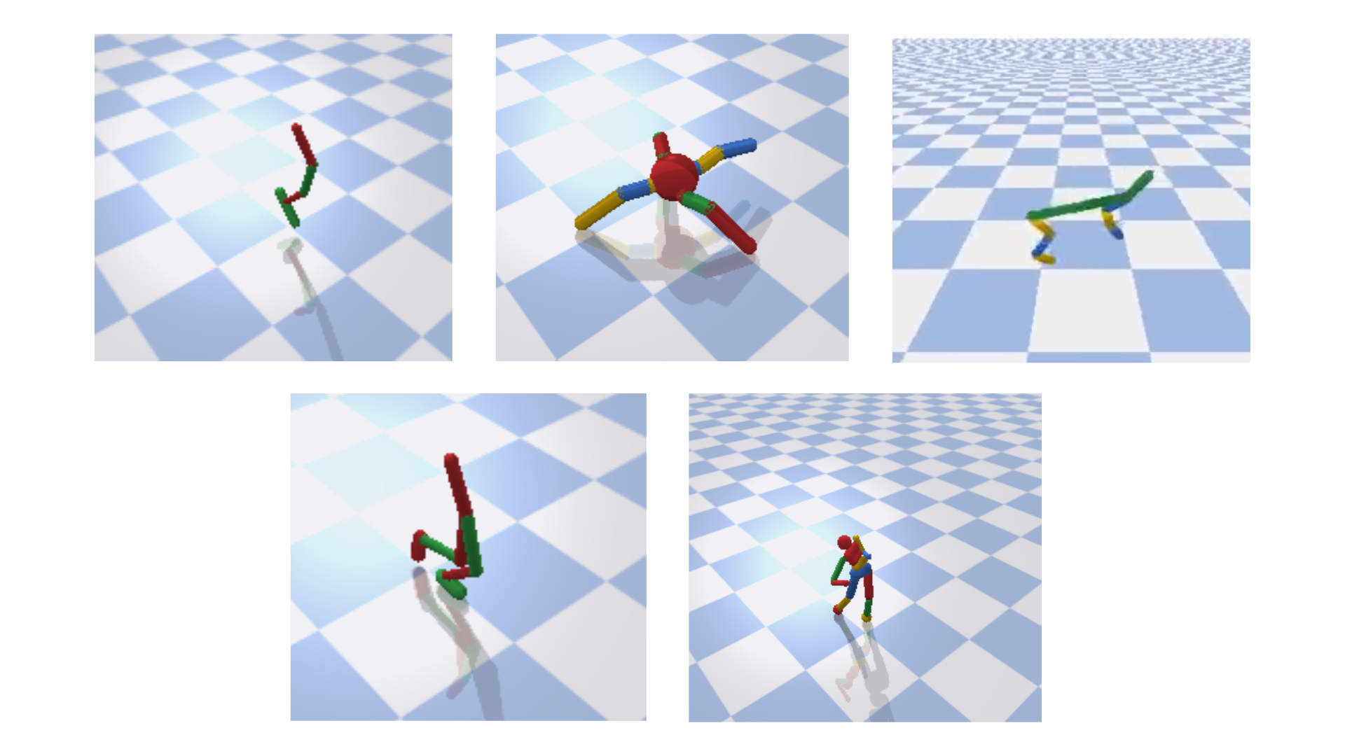
We will analyze the impact of variations in the case of the Pybullet locomotor tasks (Coumans and Bai, 2016) which involve simulated robots located on flat surfaces that should acquire the ability to jump or walk toward a given destination as fast as pos- sible. The Pybullet locomotor tasks are a standard testbed widely used to benchmark the Hopper, Ant, Halfcheetah, Walker2d, and Humanoid tasks which involve the simu- lated robots shown in Figure 1. We will use the term capitalized to indicate the task (i.e., the robot, the fitness function, and the termination conditions) and the terms without capitalization to indicate the simulated robot used in the task.

The hopper, halfcheetah, ant, walker2D, and humanoid robots have 3, 6, 8, 6, and 17 actuated hinge joints, respectively. The action vector computed by the robot’s neu- ral controller includes N values encoding the torques applied to the N corresponding joints. The observation vector, which constitutes the input of the robot’s neural con- troller, includes the position and orientation of the robot, the angular position and ve- locity of the joints, and the state of sensors that detect when a body part is in contact with another body. The initial posture of the simulated robot varies randomly within

X, X

Carvalho, J. T. & Nolfi, S. Figure 1: The hopper (top-left), ant (top-center), halfcheetah (top-right), walker2D (bottom-left) and humanoid (bottom-right) robots used in the corresponding Hopper, Ant, Halfcheetah, Walker2d, and Humanoid tasks.

a given range (see below). The evaluation episodes are terminated after 1,000 steps or, prematurely, when the torso of the robots falls below a given threshold. The fitness of the robots is computed by summing the rewards obtained during each step of the evaluation episode. The reward functions, which are used to compute the reward gained in each step, include six components: (1) a progress component that encodes the speed of the robot toward the destination, (2) a bonus for staying upright, (3) an electricity cost that corresponds to the average of the dot product of the action vector and of the joint speed vector, (4) a stall cost corresponding to the average of the squared action vector, (5) a cost proportional to the number of joints that reached the corresponding limits, and (6) a cost of -1.0 for falling down. The bonus is set to 2.0 in the case of the Humanoid and to 1.0 in the case of the other tasks. The electricity cost, stall cost, and joint at limit cost are weighted by -8.5, -0.425, and -0.1 in the case of the humanoid, and for -2.0, -0.1, and -0.1 in the case of the other tasks. A summary of the default reward functions can be seen in Table 1. As demonstrated in (Pagliuca et al., 2020), these reward functions included in the Pybullet library work well for reinforce- ment learning algorithms such as the PPO (Schulman et al., 2017) but produce poor with both the reward functions described above, which work well with reinforcement learning algorithms, and with the rewards functions introduced in (Pagliuca et al., simpler and include the first component only in the case of the Hopper and Walker2D tasks, components 1 and 5 in the case of the Halfcheetah task, components 1, 2, 4, and 5, in the case of the Ant task, and for the Humanoid task, same as Ant Task, plus two additional components which penalize by -0.1 the angular offset between the orienta- tion of the robot and the target destination, and a strong penalization of -10.0 for joints

X, X

Role of Morphological Variation in Evolutionary Robotics Table 1: Default reward functions (R-RL) components values for each task.

-1

Table 2: Reward functions components values for each task optimized for evolutionary algorithms (R-EA).

-0.1

over limits. The bonus, component 2, is set to 0.01 and to 0.75 in the case of the Ant and Humanoid tasks. A summary of the reward functions optimized for evolutionary algorithms can be seen in Table 2. We will indicate the experiments performed with the reward functions designed for evolutionary and reinforcement learning algorithms with R-EA and R-RL, respectively. Notice that the experiments reported in this article are all carried on by using the evolutionary algorithm described in section 3.2.

For more details on the tasks and on the reward functions see (Coumans and Bai, 2016) and (Pagliuca et al., 2020).

The Neural Network Controller Of The Robots

The robots are controlled with 3-layered feedforward neural networks, which means an input layer, a hidden layer including 50 internal neurons in the case of the Hopper, Halfcheetah, Ant, and Walker2d problems and 250 internal neurons in the case of the Humanoid problem, and an output layer. The activation of the internal and motor neu- rons is computed with the hyperbolic tangent (tanh) and linear functions, respectively.

The number of input and output neurons varies in different tasks and corresponds to the length of the observation and action vectors of the corresponding robot. The connection weights are encoded in free parameters and evolved with the algorithm described below.

The Algorithm

The robots are evolved by using the OpenAI-ES algorithm (Salimans et al., 2017), i.e., a state-of-the-art algorithm that belongs to the class of natural evolutionary strategies (NES) (Wierstra et al., 2014; Sehnke et al., 2010; Glasmachers et al., 2010; Schaul et al., 2011). Let F denote the objective function acting on parameters θ, the algorithm gener- ates a population with a Gaussian distribution over θ parameterized by ψ and tries to

X, X

Carvalho, J. T. & Nolfi, S. maximize the mean objective value Eθ∼pψF(θ) over the population by using the Adam stochastic optimizer (Wierstra et al., 2014). During each iteration, it takes a gradient step by using the estimator presented in equation 1.

(1)

The size of the population is set to 500 in the case of the Humanoid task and to 40 in the other tasks. The evolutionary process is continued until the total number of steps exceeds 100 million steps in the case of the Humanoid task and 50 million steps in the case of the other tasks. As in (Salimans et al., 2017) the observation vectors were normalized by using virtual batch normalization (Salimans et al., 2016, 2017), the connection weights were normalized by using weight decay (Ng, 2004), the variance of the perturbations used to generate offspring was set to 0.02, and the step size of the Adam optimizer was set to 0.01. We ran 10 replications for each experimental condition.

Easuring The Impact Of Variations

Many evolutionary algorithms rely on rank-based selection. For these algorithms, a straightforward way to measure the impact of variations on the fitness function con- sists in comparing the ranking of the fitness measures obtained during two indepen- dent evaluations. In the absence of variation, the ranking will be identical. Instead, in the presence of variation, the ranking will differ. For example, the individual that resulted the very best in the first evaluation can become the fourteen best in the second evaluation. We can measure the relative impact of variations (IV) by computing the average difference between the ranking positions obtained by each individual in two independent evaluations normalized in the range [0.0, 1.0]:

(2)

where r1i and r2i are the ranking positions of individual i in the first and in the second independent evaluation, and s is the population size. It is noteworthy that for com- pletely random generated rankings, for large population sizes, this measure follows a Gaussian distribution with an expectation of around 0.333. Therefore, we assume that the signal-to-noise ratio (SNR) is defined by the equation 3 which is defined as follow:

(3)

We refer to this measure as IV which stands for Impact of Variations. This measure is similar to the one proposed by Hansen et al. (2008) to vary the number of evalua- tion episodes allocated to each individual. As mentioned above, varying the number of episodes per individual permits allocating the computational cost required to per- form additional evaluations, especially to the individuals who are more affected by variations.

The IV can vary approximately within the range [0.0, 0.333] where 0.0 corresponds to a situation in which the variations are absent or do not have any effect on the rank- ing, 0.333 corresponds to a situation in which the ranking of the individuals reflects exclusively the effect of the variations (i.e., a situation in which the fitness measure does not provide any information about the relative ability of individuals). The value of 0.333 can be computed experimentally by computing the measure on several sets of rankings generated randomly. Therefore it is the expectation when no fitness signal is present in the rankings. It is important to consider that the IV does not depend only on

X, X

Role of Morphological Variation in Evolutionary Robotics the range of variations. It also depends on the task and on the behavioral strategy of the robots.

Overall, it is expected that the greater the range of variations, the greater the value of the IV measure. It is noteworthy though, that the agents can partially neutralize the environmental variation by acting appropriately, i.e., by executing actions that mini- mize or neutralize the effects of variations. Moreover, as mentioned above, the effect of the variations depends on the task. For example, variations affecting the shape of the objects present in the environment or the observations of the robot are expected to have a small impact on the fitness of a wheeled robot evolved for the ability to move by avoiding obstacles. Instead, the same type of variations is expected to have a significant effect on the fitness of a humanoid robot evolved for the ability to grasp objects. Finally, the IV depends on the behaviors displayed by the population of individuals. The IV measure will result in smaller or higher values depending on whether the behavior of the robots is robust or fragile with respect to morphological variations.

In the results reported below the IV is computed by evaluating the population twice every generation.

Experimental Protocol

In this section, we describe the experiments conducted to study the impact of the vari- ance of variations and of the modalities with which variations are introduced. The variations can affect the state of the robot and/or the environment at the beginning of the evaluation episodes or during each step. Moreover, we describe the experiments conducted to analyze the advantage which can be gained by increasing the precision of the fitness estimation.

Ariations Affecting The Initial State

A first type of variation concerns the initial state of the robot and/or of the environ- ment, i.e., the state at the beginning of evaluation episodes. In the case of the tasks considered, the initial state of the robot depends on the position of the joints which connect the parts of the robot’s body. In the standard implementation of the Pybullet locomotor tasks, the initial position of the joints is varied with respect to their central position with Gaussian random values which have a variance of 0.1 rad and an aver- age of 0.0 rad. In a first series of experiments, we will thus study the effect of setting the variance of this type of variation to 0.1 rad and 0.03 rad. We will use our IV mea- sure to study the impact of the amplitude of the variations on the stochasticity of the fitness. Moreover, we will analyze the impact of the distribution of variation on the performance and robustness of the evolved robots.

Ariations Affecting All States

A second type of variation concerns the effect of the motor actions performed in each step. Introducing small variations in the action vector computed by the neural con- troller of the robot is a common practice that permits taking into account the fact that the effect of physical motors is influenced by factors that are neglected in simulation, e.g., dust, wind, or small irregularities of the terrain. For example, in the experiments reported in (Salimans et al., 2017) the action vector is perturbed with Gaussian ran- dom values which have a variance of 0.01 and an average of 0.0. To analyze the effect of variations of this kind we will carry out experiments by increasing the variance of variations up to 0.6. The amplitude of the variations affecting each state can be con- stant or can vary during the course of the evaluation episode or across generations.

X, X

Carvalho, J. T. & Nolfi, S. We will investigate the effect of the modality with which variations are introduced by analyzing the following experimental conditions: (i) a fixed condition in which the range of variations is constant and is set to 0.01, 0.3 or 0.6 (ii) an incremental condition, referred as inc-episode, in which the variance of variations increases linearly during the course of the evaluation episode up to 0.36 or 0.55, and (iii) a second incremental condition, referred as inc-generation, in which the variance of variations increases lin- early across generations up to 0.55. The rationale behind the inc-episode condition is that it reduces the risk to generate solutions overfitted to a specific range of variation.

Moreover, it produces a form of incremental process which exposes low-performing robots, which fall down rapidly, to variations that have a small variance only and high- performing robots also to variations that have a high variance. The rationale behind the inc-generation condition is also the generation of an incremental process. Indeed, it exposes the robots of the first generations, which typically display low performance, to variations with a small variance and it exposes the robots of successive generations to variations that have a higher variance.

The variations described above and in the previous section are applied to all evolv- ing individuals, i.e., to the entire population.

Mproving The Precision Of The Fitness

As mentioned above, the accuracy of the fitness can be improved by using the average value obtained during multiple evaluation episodes in which the robots are exposed to different variations.

This method is computationally expensive since evaluation episodes represent the major computational cost. To analyze the advantage which can be gained through this method we will report the results of a series of experiments in which the number of evaluation episodes is set to 1, 2, 3, 5, and 10. For the purpose of our comparison, we neglect the computation cost caused by the execution of multiple episodes. This is realized by multiplying the maximum number of evaluation steps by the number of episodes. This implies that the experiments carried out by performing 2 and 10 evaluation episodes, for example, last approximately twice and 10 times more than the experiments carried out by performing a single evaluation episode.

Replicating The Experiments

The experiments can be replicated by using the source code and the instructions avail- able from the following repository: ”https://github.com/snolfi/env-variation”.

Results

In this section, we report the results obtained after conducting the experiments pre- sented in the previous sections. We start by analyzing the impact of the variations affecting the initial state. We analyze the advantages which can be gained by increas- ing the accuracy of the fitness measure. Finally, we analyze the impact of the variations introduced in each step and the modality with which those variations are introduced.

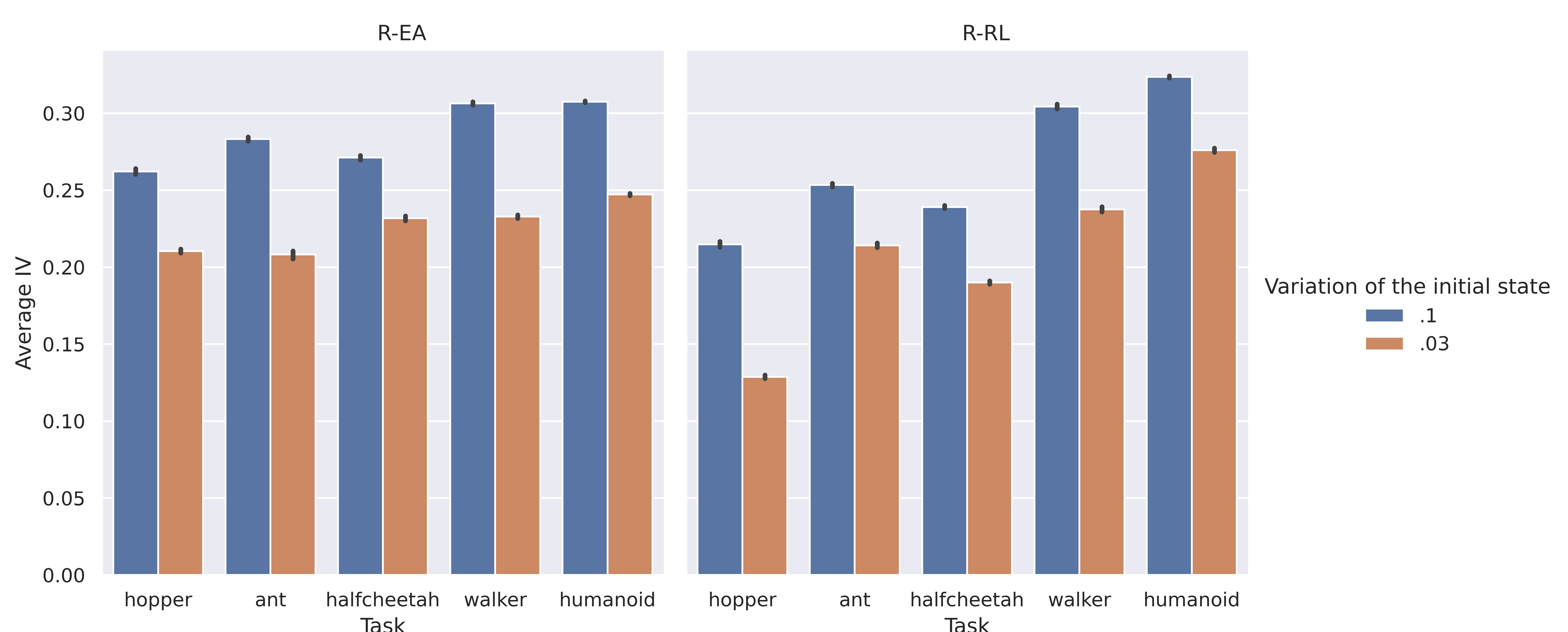
On the impact of variations affecting the initial state Figures 2 and 3 display the IV and the performance obtained in experiments in which the variance of variations affecting the initial state of the robots is set to 0.1 rad and 0.03 rad, respectively. The variance of variations affecting the action vectors is set to 0.01, i.e., to a small value. The figures on the left and on the right report the results obtained with the reward function designed for evolutionary and reinforcement learn-

X, X

Role of Morphological Variation in Evolutionary Robotics ing algorithms, respectively. The performance of the evolved agents was computed by post-evaluating them for 10 episodes.

Figure 2: IV for the Hopper, Halfcheetah, Ant, Walker2d and Humanoid tasks. The data shown in blue and orange display the data obtained by using a distribution of 0.1 rad and 0.03 rad to perturb the initial state of the robots, respectively. Values averaged over generations and over 10 replications. Left: experiments performed with the reward function designed for evolutionary algorithms (R-EA). Right: experiments performed with the standard reward function designed for reinforcement learning algorithms (R-

Rl).

The analysis of the performance and the inspection of the behavior of the agents evolved with the reward function designed for evolutionary algorithms (Figure 4, left) show that they display an effective walking behavior in all cases with the exception of the Humanoid task in which the robots fail to walk in the experiments in which the variance of the variations of the initial posture is 0.1 rad. Reducing the amplitude of the variations to 0.03 rad enables the evolving robots to develop effective behaviors also in the case of this task in most of the replications.

The robots evolved with the reward function designed for reinforcement learning, instead, develop a sub-optimal behavior in most of the replications which consists in quickly assuming a posture from which they can remain still without moving (Figure 4, right). Such behavior maximizes the reward bonus received for not falling down but fails to maximize the reward that the robots could potentially receive by jumping or walking forward. In this case the reduction of the distribution of variations to 0.03 rad produces better performance in the case of the Ant, Halfcheetah and Humanoid experiments (Figure 4, right, orange data). As we will see in the next section, the con- vergence of the evolving robots on the suboptimal behavior which consists in staying still depends also on the variance of the variations applied to the action vector in each step.

The IV is generally quite high and correlates with the complexity of the problem (Figures 2 and 3). Indeed, it is higher in the case of the Walker and Humanoid tasks which are more difficult than the other three tasks. The higher difficulty of the former tasks is demonstrated by the fact that performance increases more slowly throughout generations. In the experiment with the fitness function designed for evolutionary al- gorithms and in which the variance of variation is set to 0.1 rad the signal-to-noise ratio (SNR) ranges from 25%, in the case of the hopper, to 3% in the case of the humanoid.

Authors:

Peder EZ Larson 1, 2,* , Jenna ML Bernard1, James A Bankson 3, Nikolaj Bøgh 4, Robert A Bok1, Albert P. Chen 5, Charles H Cunningham 6,7, Jeremy Gordon1, Jan-Bernd Hövener 8, Christoffer Laustsen 4, Dirk Mayer 9,10, Mary A McLean11 12, Franz Schilling13, James Slater1, Jean-Luc Vanderheyden5, 14, Cornelius von Morze 15, Daniel B Vigneron1, 2, Duan Xu1, 2, and the HP 13C

94143, Usa.

Denmark. 5 GE Healthcare, Menlo Park, California, USA. 6 Physical Sciences, Sunnybrook Research Institute, Toronto, Ontario, Canada.

8 Section Biomedical Imaging, Molecular Imaging North Competence Center (MOIN CC), Medicine, Baltimore, MD, USA. Cambridge, United Kingdom.

14Jlvmi Consulting Llc, Dousman, Wi, Usa

#See Acknowledgements for a list of all HP 13C MRI Consensus Group Members This work was supported by the ISMRM Hyperpolarized Media MR Study Group, the ISMRM Hyperpolarization Methods & Equipment Study Group, and the Hyperpolarized MRI Technology Resource Center (NIH/NIBIB grant P41EB013598).

Abstract

MRI with hyperpolarized (HP) 13C agents, also known as HP 13C MRI, can measure processes such as localized metabolism that is altered in numerous cancers, liver, heart, kidney diseases, and more. It has been translated into human studies during the past 10 years, with recent rapid growth in studies largely based on increasing availability of hyperpolarized agent preparation methods suitable for use in humans. This paper aims to capture the current successful practices for HP MRI human studies with [1-13C]pyruvate - by far the most commonly used agent, which sits at a key metabolic junction in glycolysis. The paper is divided into four major topic areas: (1) HP 13C-pyruvate preparation, (2) MRI system setup and calibrations, (3) data acquisition and image reconstruction, and (4) data analysis and quantification. In each area, we identified the key components for a successful study, summarized both published studies and current practices, and discuss evidence gaps, strengths, and limitations. This paper is the output of the “HP 13C MRI Consensus Group” as well as the ISMRM Hyperpolarized Media MR and Hyperpolarized Methods & Equipment study groups. It further aims to provide a comprehensive reference for future consensus building as the field continues to advance human studies with this metabolic imaging modality.

Keywords: Hyperpolarized MRI, metabolic imaging, carbon-13, pyruvate, dissolution dynamic

Introduction

MRI with hyperpolarized 13C agents, also known as hyperpolarized (HP) 13C MRI, has shown great potential as a novel imaging modality, particularly for its ability to probe metabolic processes in real time. The first human studies with HP [1-13C]pyruvate were performed in 2011 in prostate cancer patients (1).

Since then, there have been over 60 papers published with imaging results of human subjects from 13 different sites, with applications including prostate cancer, brain tumors, breast cancer, kidney cancer, pancreatic cancer, metastatic disease, liver disease, ischemic heart disease, diabetes and cardiomyopathies. The vast majority of these studies used [1-13C]pyruvate (1–63), where [2-13C]pyruvate (64) and 13C-urea (56) have been demonstrated too.

As clinical HP 13C MRI advances, there is a growing need to build consensus for best practices, which are critical for comparing data across sites, performing multi-site trials,deploying methods to new sites, partnering with vendors, and potentially for obtaining broader regulatory approvals.

In March 2022, we initiated an effort to build consensus within the HP 13C MRI community with this opportunity in mind, and it was greeted with strong enthusiasm. The “HP 13C MRI Consensus Group”, containing over 55 members from 27 sites, identified the area of greatest need and opportunity for consensus building to be HP [1-13C]pyruvate human

●

Pyruvate is the most mature and widely used HP agent and has the most significant translational evidence emphasizing the potential clinical impact.

●

Clinical trials, particularly multi-site trials, have the strongest need for consensus methods to ensure that data can be combined across sites. This work is a Position Paper for which the goal is to describe current successful practices and study methods for HP [1-13C]pyruvate human studies along with justification to support those practices. This is divided into four major topic areas: (1) HP 13C-pyruvate preparation, (2) MRI system setup and calibrations, (3) data acquisition and image reconstruction, and (4) data analysis and quantification (Fig. 1). The current successful practices and study methods include a literature review of published peer-reviewed journal papers showing human HP [1-13C]pyruvate study data, up to September 2022 (1–63), as well as new unpublished information from surveys of HP 13C study sites. Based on this information, we also highlight the evidence gaps, strengths, and limitations of current practices which are summarized at the end of each section.

Figure 1: Illustration of the HP 13C MRI human study process, including the 4 major areas covered in this paper: Hyperpolarized 13C-pyruvate preparation, MRI system setup and calibration, Acquisition and Reconstruction, and Data Analysis and Quantification.

Figure 2: Anatomical targets of HP [1-13C]pyruvate MRI human studies published up to September 2022.

Hyperpolarized 13C-Pyruvate Preparation

This section covers the processes for creating the HP agent, 13C pyruvate, and will include many aspects and considerations that are needed to safely and effectively prepare doses for metabolic imaging studies in human subjects. These include material, personnel, equipment and facility, fluid path preparation, quality control, and release.

It is helpful to understand that the specifications of a dose of 13C pyruvate suitable for in vivo MR HP metabolic imaging were shaped in part by early preclinical studies performed by GE HealthCare summarized in Ref. (65). In short, the safety of the two novel drug components, 13C pyruvate and the electron paramagnetic agent (EPA) AH111501, were demonstrated in those studies. The more precise formulation of the dose suitable for human use was then determined from clinical studies (66) that included two Phase 1 clinical trials in young and elderly healthy volunteers without hyperpolarization of the 13C nuclei and another Phase 1/2a dose escalation and imaging feasibility study with HP 13C pyruvate in 31 prostate cancer patients at the With the exception of the first HP 13C imaging clinical trial, which utilized a prototype device in a cleanroom (1), all HP 13C studies performed in humans to date have utilized the SPINlab polarizer (manufactured by GE HealthCare). Consequently all doses of the HP 13C pyruvate delivered by SPINlab have been produced using the “SPINlab Pharmacy Kit” that serves as the container-closure system for the various drug components (13C pyruvic acid and EPA mixture, dissolution medium, and neutralization and dilution medium) during sample polarization, dissolution and quality control (QC) processes. Thus many aspects of the HP sample preparation considerations discussed below are related to the SPINlab instrument and the consumables designed to be used with it (67).

General Considerations

While more than 860 patients or healthy subjects having been injected with HP 13C pyruvate as of January 2022 without reports of any serious adverse events (68), HP 13C pyruvate injection remains an investigational MR contrast agent and can only be administered by those with Investigational New Drug (IND) exemption from the Food and Drug Administration (FDA) in the USA, a Clinical Trial Application (CTA) in Canada, approval from National Research Ethics Committee Services in the UK, or approval from the relevant local regulatory body. Thus, methods and processes involved to produce a dose should have patient safety as the first priority. Since utilizing dissolution dynamic nuclear polarization (dissolution-DNP) for human use is still a relatively new development, there are no existing published regulatory guidelines specifically for this method.

There are two major production styles that determine how various sites approach the agent preparation. In the US, the most common approach is to rely on a sterilizing filter (“Terminal Sterilization”) to ensure sterility of the final product, akin to PET tracer production, where a starting molecule with a radioisotope is processed using various other ingredients to make the final, desired and injectable contrast agent within a necessarily short amount of time (69). For these sites, sterilization of the components and accessories upstream of this filter are not required, although many of them were manufactured and tested following Good Manufacturing Practice (GMP) or Good Laboratory Practice (GLP) requirements. The filling process is usually performed under an ISO 5 laminar flow hood, but a clean room or an isolator is not required.

This approach is typically accompanied by testing the integrity of the sterilizing filter prior to release of the dose for injection. Typically, post release endotoxin and sterility tests are performed using an aliquot reserved from each released dose.

In the UK and EU, the most common approach is to more-closely follow sterile pharmaceutical compounding guidelines (70), where all components and ingredients are required to be sterile or manufactured under GMP guidelines and are assembled and filled within a clean room environment or an isolator system (“Sterile Preparation”). Typically a batch of Pharmacy Kits for HP 13C pyruvate injection are prepared together. The sterility of the final dose is also ensured by batch validation testing, in addition to the sterility of the ingredients and the sterile compounding process. The endotoxin and sterility testing are performed for the process validation but are not performed for each injected dose.

Some institutions fill and assemble the Pharmacy Kit required for a specific study on the same day or the day prior to polarization, dissolution, and patient administration, but others have also demonstrated the feasibility of preparing a batch of kits, keeping them in a -20ºC freezer and using them over a period of a few months.

Beyond the obvious requirements that the process and the facility has to ultimately produce a dose that is safe to inject into a human, regulatory authorities will also focus on the question “Are you in control of your processes?”. To be in control of your process requires an in-depth and broad understanding of all processes involved in pre, post, and during the production process.

Personnel

It is typical and may be required to have licensed personnel involved in the production process depending on local regulations.Typically a pharmacist, radiopharmacist or other similarly qualified person (QP), in charge of the facility where the Pharmacy Kit filling and preparation is taking place, is responsible for the overall process and the release of the injectable dose.

Qualified cleanroom technicians are often involved in the Pharmacy Kit filling under the supervision of the pharmacist or QP. As is required for pharmaceutical compounding or PET tracer production, training requirements and training records for all personnel need to be maintained and available for audit by the FDA or equivalent.

Equipment And Facility

The facility and all equipment need to have standard operating procedures (SOPs) that describe how equipment is used, maintained, and calibrated to comply with relevant legislation. Currently, almost all the filling of the Pharmacy Kit takes place within a compounding laminar flow hood or isolator (typically ISO 5). At some sites, the filling is conducted within a cleanroom, while at others, it is conducted in a dedicated non-cleanroom space, reflecting differences in cleanroom approach and specifications between regulators worldwide (71). Some equipment or facilities, such as the compounding hood or cleanroom, may require external certified laboratories for testing.

Material Handling

Material handling guidelines (69,70) require SOPs detailing a system to track all of the materials involved in the HP production process for a particular patient dose, similar to current good manufacturing practice (cGMP) requirements for material handling for drug compounding. This includes acceptance standards, storage conditions, amount used in the patient dose for each ingredient and materials used in the assembly of the fluid path and Pharmacy Kit. Currently some users choose to open and inspect and sometimes modify the Pharmacy Kits upon arrival, but some users keep them in the sealed packaging until they are required for dose preparation.

Pharmacy Kit Filling And Assembling

As required by an IND or its equivalent, the preparation of the doses of HP 13C agent are detailed in the Chemistry, Manufacturing, and Control (CMC) section of an applicable regulatory submission; an example of this has been made available (72). It describes the processes of filling the Pharmacy Kit with the different components that make up the final drug product, and of assembling the final kit for either storage or immediate use in the polarizer. Special attention should be given to the laser welding process in order to satisfy installation qualification (IQ) and operational qualification (OQ). Typically, the final developed process is validated by process qualification (PQ) runs, during which 3 or more Pharmacy Kits are filled and used and the final HP 13C products are tested for endotoxin and sterility and to confirm that they meet the dose specifications for injections (usually including pyruvate concentration, residual EPA concentration, pH, liquid state polarization level and dose temperature). The data from 3 consecutive PQ runs are submitted as part of the IND submission (or its equivalent), and are often also reviewed by the Institutional Review Board (IRB) where the studies are conducted.

Quality Control And Dose Release

The quality control (QC) and dose release can be separated into two aspects: one is the QC and release of the filled Pharmacy Kit, and second is the QC and release of the HP 13C agent for injection, after polarization and dissolution. For institutions filling a batch of kits and storing them to use over a period of time, typically the batch can be released based on initial validation, environmental monitoring data from the day of kit production, and if filters are used during preparation of any of the components, filter integrity testing. But in some cases one or more kits are used for validation before the batch of kits are released for future use. For institutions that fill only the kits required for specific studies shortly before the experiment, the filled kits often do not go through separate release tests before they are used.

The quality control of the HP 13C pyruvate solution post dissolution is primarily performed to ensure that the agent meets the dose specifications (Table 1) before it is administered to the subject. These specifications target both safety (pH, residual EPA, temperature) and efficacy (pyruvate concentration, polarization, volume). Typically, the pyruvate concentration, residual EPA concentration, pH, dose temperature, dose volume, and liquid state polarization are measured by the QC accessory associated with the SPINlab polarizer. Some users perform a secondary measurement for one of the parameters, such as pH, using a different instrument or pH paper. For sites that do not go through a separate release testing process for batch filled kits, the integrity of the sterilization assurance filter, a part of the Pharmacy Kit, is typically tested as a part of the dose release. It is also common for these users to preserve an aliquot of the final HP 13C pyruvate solution for post-release endotoxin and sterility testing. This testing cannot be completed fast enough to test an individual dose prior to injection, but this is why other processes such as PQ runs and validation testing are done to minimize the chance a subject could be injected with a contaminated dose.

The Final Dose Release And Injection

should be done under the supervision of a licensed professional, based on local regulations.

Some Key Challenges

Many of the challenges associated with HP 13C pyruvate preparation can be attributed to the conditions required for the dissolution-DNP method of high magnetic field (~3-7 T) and very low temperature (~1 K) during polarization, with pressurized and superheated water necessary for the rapid dissolution event. These extreme conditions are quite challenging for the design of the container-closure and fluid path system. In particular, the cryogenic temperature in the polarizer requires special attention to any moisture or ambient (moist) air introduced into that portion of the fluid path, which can form an ice block at ~1 K. This ice can lead to flow restriction during the dissolution event and reduce the strength of the laser welded bond between the cryovial and its cap. This can ultimately produce failures in the dissolution step, including variations in final pyruvate concentration and pH that may fail to meet QC release criteria as well as fluid path ruptures that provide no available dose and result in polarizer down-time.

The polarization of the HP 13C pyruvate sample decays quickly over the span of a few minutes after dissolution, and thus the process of dissolution, QC for release, and injection should be completed as fast as possible to preserve the high polarization level achieved. Any delays in the preparation process, such as transportation time or equipment malfunction, can significantly reduce the final polarization and result in lower quality imaging data.

Current Practices

A summary of data collected from all sites performing clinical trials with HP 13C-pyruvate is shown in Fig. 3 and Table 1, including the specification of the final dose and how the quality control and release of the final dose are performed. There is a split in the Production Style, described in the General Considerations section above, with 8/13 sites using Sterile Preparation versus 5/13 using Terminal Sterilization. While many of the dose specifications show notable differences in acceptable ranges, all of these variations listed in tables have been successfully and safely been used to perform HP 13C pyruvate studies in humans. Their differences depend on the institutions’ preferences, resources and their particular regulatory situation. There is high similarity in pyruvate ranges, temperature ranges, EPA limits, and volume limits. There is modest variability in pH ranges and large variability in the endotoxin test limit. There is a 3-fold difference in acceptable polarization levels, which are measured to ensure a futile dose is not injected since the polarization is directly proportional to SNR. This reflects the decision by several sites to believe that useful data can be still be obtained with suboptimal polarizations.

Figure 3: Hyperpolarized agent preparation methods reported by sites currently performing HP

In House

Table 1: HP 13C-pyruvate preparation parameters, methods, and dose specifications used for quality control testing and release as well as validation. These were obtained from a survey of all sites performing clinical trials with HP [1-13C]pyruvate. The parameters used for product release are noted in bold text, otherwise these parameters are measured for batch validation or other QC measurements. The endotoxin and sterility testing are performed during process validation of the batch and/or post-injection, and largely depends on the agent production approach.

Summary

The overall safety record of HP 13C-pyruvate has been very strong, and the SPINlab hyperpolarizer has proven to provide high polarizations at human sized doses while meeting numerous QC and release criteria. A weakness remains the failure modes of the SPINlab Phamacy Kits (e.g. ice blocks, path ruptures), which are placed under extreme requirements particularly during dissolution. The preparation process still requires a high degree of expertise.

Therefore, there is a significant need to improve the reliability, robustness, and ease of operation for generating HP 13C-pyruvate doses for human studies. Furthermore, there is a divide between manufacturing and sterile compounding style preparation as well as other site-specific practices, resulting in variations in SOPs and justification required to relevant regulatory bodies. There have also been no comparisons between these approaches. It is also unclear what release criteria and QC parameters are truly required to ensure patient safety.

However, all of the reported methods are acceptable and approved by the appropriate regulatory authorities, and have led to the rapid expansion of successful human studies in recent years.

Mri System Setup And Calibrations

This section covers the MRI system setup, including the imaging system, RF coils, phantoms, and prescan calibration methods.

Imaging System

The main prerequisite for a given MRI scanner to be capable of supporting studies with HP 13C is its “broadband” capability to transmit and receive radiofrequency (RF) signal at the frequency of 13C, which is around 4 times lower than 1H. This does not come as a default on clinical MR devices. The transmit power of the broadband amplifier should also be sufficient to support the intended flip angle and RF pulse shape with the employed transmission RF coil(s) for 13C. Most studies to date use relatively low flip angles (< 90 degrees) for HP 13C in order to preserve polarization for time-resolved imaging. The capability to receive 13C signal on multiple channels is also desirable to increase SNR, as discussed further in the “RF coils” section.

The choice of magnetic field strength is primarily dependent on the metabolites’ frequency separation due to chemical shift dispersion and 1H imaging. High field strengths do not enhance hyperpolarized 13C signal as they do for 1H because the signal strength in a HP experiment relies on manipulating the population of quantum energy states outside of the MRI scanner.

However, the injected HP 13C-pyruvate and its metabolic products have greater frequency separation at higher fields, and it may thus be easier to separate and quantify these resonances at higher fields. This comes at the cost of a reduction in the achievable T2* and often reduced T1. As the initial polarization is independent of the imaging field strength it has been proposed that the increased T2* at 1.5T can potentially be exploited to increase SNR by adapting the acquisition bandwidth or reduce off-resonance imaging effects in cases when the decay of the transverse magnetization is dominated by T2* (73). In practice, 3T has been used in all published human 13C-pyruvate studies surveyed (Supporting Table S1), and comprises the majority of scanners currently in use for human studies (Table 3). A field strength of 3T is well-suited for 1H MRI anatomical reference and correlative imaging.

Stronger and more rapidly slewing magnetic field gradients support more rapid spatial encoding, particularly for metabolite-specific single-shot imaging using echo-planar imaging (EPI) or spiral imaging (See “Acquisition and Reconstruction”). Although the spatial resolution acquired for HP 13C imaging is typically much coarser than for 1H MRI, the factor of ~4 in gyromagnetic ratio leads to the same reduction factor in performance of the gradient system, so 13C experiments are potentially more limited by gradient hardware performance. To date, all human studies have used the commercially-available integrated gradient systems provided in clinical MRI scanners.

Optimization of scanner design has understandably focused on minimization of artifacts in 1H MRI, where devices such as room lights, the gradient amplifiers, and the motors driving the patient bed are checked to ensure that they do not produce RF interference at the 1H frequency, but artifacts may arise at other frequencies. Eddy current compensation is also not always appropriately adjusted for nuclei at other frequencies (74). In order to optimize for 13C, many sites have performed checks on phantoms for RF interference, gradient artifacts, and eddy currents (74), including the use of post-hoc gradient impulse response function characterisation and correction, and some vendors have fixed these issues as well.

Rf Coils

For HP 13C imaging studies in humans, RF coils for both 1H and 13C nuclei are needed, with 1H MRI providing an anatomical reference for registration and optional additional multiparametric MRI readouts. At the Larmor frequency of 13C nuclei, the relative contributions from coil noise compared to sample noise increase compared to 1H (73,75), although sample noise still is likely the dominant contributor for human-sized coils at 32.1MHz - the resonance frequency of 13C nuclei at 3T.

The key requirement for human 13C-pyruvate RF coils are that the coil geometry and sensitive volume must cover the volume of interest in the subject. Table 2 and Figure 4 shows coil configurations that have been used and optimized for applications in different anatomic regions.

Volume resonators are most commonly used for transmit, as they surround the subject to

Provide B1 Transmit Across The Fov (B1

+). While 1H relies on a large birdcage (“body”) coil built into the scanner, 13C transmit coils must be placed inside the bore. This takes up valuable space within the magnet, and also has led to the use of designs with relatively inhomogeneous

B1

+. Many human studies have used Helmholz pair resonators for transmit, including the “clamshell coil”, which has a notably inhomogeneous B1

+ Profile But Has Been Used Because Of

relatively easy integration into the scanner bore. B1

+ Variation Results In Variations In The Flip

angles that control the use of the hyperpolarized magnetization and creates errors in common HP metrics (9,76). The exception are head coils, where birdcage designs with highly

Homogeneous B1

+ can be placed around the head while easily fitting inside the bore. As with 1H MRI, higher SNR can typically be achieved by smaller receive coil elements, such as surface coils or phased arrays, and the majority of 13C receive coils used have layouts similar to 1H phased arrays.

RF coil quality control is important to ensure proper functioning of the coils to provide consistent imaging quality, especially with limited natural abundance 13C signal in vivo. It typically involves 1) a physical integrity check of the coil cables and connectors and 2) phantom SNR tests to check the coil’s performance and to monitor it over time (see Phantoms below). An useful reference for RF coil quality control is outlined in the MRI accreditation program of the American College of Radiology (77) and can be adapted for 13C coils.

Notably, configurations for brain and prostate studies used dual-tuned 1H/13C coil designs, which greatly simplify workflow and registration of 1H and 13C images, as no switching of coils is needed.

(1)

Table 2: RF coil configurations reported for human HP [1-13C]pyruvate studies.

Tx = Transmit

coil, RX = receive coil. The commonly used “clamshell” TX coil is a Helmholz pair design. For 1H RF configurations, all used the Body coil for TX unless otherwise noted, and “repositioned” indicates the 13C coil was removed for 1H imaging. One representative reference is listed for each configuration. The RF coil configurations reported in the reviewed papers are shown in Supporting Table S1.

Figure 4: Examples of RF coil configurations used for human HP [1-13C]pyruvate brain studies. (A,B) 13C Clamshell TX (Helmholz pair) and 2× 4-channel paddle RX arrays. (C) 13C Birdcage volume TX and 32-channel RX array (RX array slides into TX coil). (D) 13C Birdcage volume TX and 24-channel RX array, combined with a 1H 8-channel RX array. Image reproduced with permission from Ref (16).

Phantoms

Since hyperpolarized magnetization is non-renewable, phantoms containing 13C nuclei are important to: 1) test the multi-nuclear capabilities of the imaging system, including all parts of the signal excitation and receive chain; 2) perform calibration measurements before a scan with hyperpolarized nuclei; and 3) perform necessary pre-scan adjustments (see “Prescan Calibration” section). The phantoms currently in use are listed in Table 3. Their composition must provide sufficient 13C signal, with additional considerations of conductivity, stability, chemical shift(s) present, potential for dynamic imaging, and cost. The phantom geometries are typically either compact, in order to be used alongside the subject during a HP scan, or large enough to mimic the inner volume of a RF coil for system testing.

One popular compact design contains enriched 13C-urea at high concentration, typically 8 M, which provides a single resonance, placed inside a small container ~1 mL. The most common recipe mixes 13C-urea in a 90% water/10% glycerol solution, with glycerol used to increase the urea solubility and doping with a Gd-based contrast agent to shorten T1 which increases the potential SNR per unit time. For example, when Dotarem is added at a 3:1000 volume ratio the 13C-urea T1 is around 500 ms and T2 is around 100 ms. However, when testing pulse sequences influenced by T1 and T2, doping should be used carefully. This phantom is suitable for frequency calibration, transmit gain calibration, sequence testing, and as a fiducial marker when placed next to a patient. However, enriched 13C-urea has a relatively high cost compared to natural abundance compounds.

For larger volumes (>100 ml), the phantoms most often used contain undiluted ethylene glycol, glycerol, or dimethyl silicone. These compounds have sufficiently high carbon concentrations to provide sufficient 13C signal even with the 1.1% natural abundance of 13C. These larger phantoms matching the inner volume of an RF coil are useful for coil testing, including transmit

+) And Receive (B1

-) coil profile mapping, as well as to mimic acquisitions using in vivo FOV requirements. In this case, size and conductivity should match the expected subject size in order to mimic coil loading and get a realistic estimation of B1+. Large-volume natural abundance urea phantoms have also been used by some sites, but suffer from higher conductivity compared to biological tissues. Typically, it is easier to increase the conductivity and hence coil loading of the non-conductive phantom by adding NaCl to match physiological loading (16,78).

Dynamic phantoms that aim to mimic metabolite kinetics have also been developed (79–81), and have the potential to more closely mimic the HP experiment, but so far these are not widely used.

Prescan Calibration

Prior to performing an MRI acquisition, the so-called prescan procedure is used to set the shim parameters to maximize B0 homogeneity over the field of view (FOV) or a specific region of interest (ROI), the scanner center frequency (CF), the RF transmit gain, and the receiver gain.

While this calibration procedure is usually automated for 1H, the lack of sufficient natural abundance 13C signal prevents use of automated methods. (Although natural abundance 13C lipid signal has been detected, there are so far no reports on using this signal for prescan.) Table 3 shows current practices across sites.

Maximizing B0 homogeneity is independent of the nucleus and is therefore performed prior to 13C imaging using the 1H water signal and existing shimming tools, such as by a standard automated process (“Auto Shimming”) or using high order shimming routines. Similarly, the 13C CF can be calculated from the 1H CF using a predetermined scaling factor that depends on the target chemical shift (82). Another common approach used is to have a small, high-concentration 13C phantom, e.g. 8M 13C-urea, integrated in the RF coil or placed next to the scan subject (1). The reference frequency can also be based on real-time measurements after the HP injection but prior to imaging (83). Both the CF and B0 shimming are critical when using spectrally-selective RF pulses, as inmetabolite-specific imaging methods, where the desired excitation bandwidths are typically very narrow and frequency offsets can lead to a failure mode that is only apparent after injection.

The calibration of the RF transmit power is typically performed on a small, high-concentration 13C phantom placed near the region of interest during the scan or on a large 13C phantom of similar size and coil loading as the subject, prior to the subject scan. Reference power is often done by sweeping the power in a pulse-acquire sequence (53,62), or the Bloch-Siegert method (52,84). When using a small phantom, the location of the phantom, B1

+ Inhomogeneity As Well

as any shielding effects, e.g., when the phantom is integrated into a coil (1), may degrade the accuracy. Other methods include real-time Bloch-Siegert method measurements after the HP injection (83), and using the stronger natural abundance 23Na signal that is close enough to the 13C resonance frequency to be detected by 13C coils (82).

The receiver gain is predetermined, either systematically based on independent phantom measurements and assuming the dose and polarization of the HP compound is known prior to injection, or based on past HP imaging studies.

Power [Kw]

Phantom(s) - during study Phantom(s) - before study 13C Frequency

8

13C-bicarbonate doped with dimethyl silicone, various

Power [Kw]

Phantom(s) - during study Phantom(s) - before study 13C Frequency

Maximum Values

Table 3: Summary of the imaging systems, phantoms, and prescan procedures used at sites currently performing HP 13C-pyruvate human studies. These were obtained from a survey of all sites performing clinical trials with HP [1-13C]pyruvate. *Previously performed studies with a Siemens 3T Tim Trio. The imaging systems, phantoms, and prescan procedures reported in the reviewed papers are shown in Supporting Table S1.

Summary

Commercially available 3T MRI systems are by far the most commonly used for human HP 13C-pyruvate studies, although a systematic investigation of the impact of B0 has only recently been investigated (73). The multi-nuclear RF transmit and receive chain has proven sufficient for current acquisition strategies, although many sites have observed artifacts due to RF interference, gradient interference, and residual eddy currents when operating at the 13C frequency. A variety of 13C RF coils, tailored for numerous anatomical targets, have been successfully demonstrated, with the main limitation that most transmit coils take up a lot of additional space inside the bore and provide relatively inhomogeneous B1

+ Profiles. The

phantoms used have converged into generally 2 categories - small phantoms containing 13C-enriched compounds that can be used during the study and human-sized phantoms containing compounds with high carbon concentrations but without 13C enrichment that are used to test and calibrate the coils. There are no standardized compositions or geometry, and dynamic phantoms that recapitulate in vivo kinetics would be desirable but are still an emerging area. Prescan calibration procedures were not well defined in most publications, so we surveyed individual sites to determine current practices. Calibration procedures for the B0 field (13C CF and shimming) for most sites take advantage of 1H signal and methods, while methods

For Calibration Of B1

+ is more variable across sites, likely a reflection of remaining challenges in how to perform this calibration. Standardization of both phantoms and calibration procedures would synergistically improve the robustness and reproducibility of HP 13C studies.

Acquisition And Reconstruction

Data acquisition strategies in human HP [1-13C]pyruvate MRI studies must account for multiple chemical shifts, efficiently utilize the non-renewable HP magnetization, and acquire data quickly relative to metabolism and relaxation decay processes. These studies require spectral encoding to separate metabolites, necessitating pulse sequences that efficiently encode up to 5D data (3 spatial + 1 spectral + 1 temporal dimension). RF pulses must efficiently sample without immediately saturating the non-renewable HP magnetization, and sequences must acquire data quickly and be robust to both experimental and physiologic variation (e.g. B1

+ Inhomogeneity,

variation in perfusion) to ensure reproducibility and minimize scan-to-scan variability. This section covers current successful practices for data acquisition in human [1-13C]pyruvate studies, and accompanying 1H imaging, from different anatomic regions, including scan parameters and image reconstruction.

Acquisition And Reconstruction Methods

The acquisition methods used in human [1-13C]pyruvate studies can be classified into 3 categories: 1) MR spectroscopy or MR spectroscopic imaging (“MRS/I”), 2) chemical shift encoding methods, and 3) metabolite-specific imaging (Fig. 5).

Mrs/I Methods Specifically

resolve a spectrum that can be analyzed to extract expected as well as unexpected resonances, making this approach very robust. It was used in many initial studies (1).

Chemical Shift

encoding methods, most commonly the Iterative Decomposition of water and fat with Echo Asymmetry and Least-squares estimation (IDEAL) method, use imaging sequences acquired with multiple TEs and rely on a model-based separation of expected chemical shifts (85).

Metabolite-specific imaging methods use specialized RF pulses that are spatially and spectrally selective to excite individual metabolites which are then typically imaged with fast k-space trajectories such as echo planar imaging (EPI) or spirals (86).

Their Application To Different

organ systems is described below. The image reconstruction methods used in human [1-13C]pyruvate studies have typically been conventional methods (e.g. FFT, non-uniform FFT, or equivalent). The incorporation of accelerated imaging and advanced reconstruction methods including parallel imaging (4,57,87) and compressed sensing (7) has also been applied in human studies for improved spatial resolution, temporal resolution and coverage, but have the potential for additional artifacts as well as SNR losses due to ill-conditioning of the reconstruction (e.g. g-factor).

The Majority Of

published studies do not use accelerated imaging indicating the resolution and coverage achievable without acceleration is currently adequate for successful data collection. Performing coil combination, even with fully sampled data has also been shown to have specific challenges for HP human images: using naive sum-of-squares methods suffer from high noise amplification in the relatively low SNR regime of HP [1-13C]pyruvate (compared to 1H), motivating several HP 13C-specific methods that include data-driven coil sensitivity estimation which have shown obvious improvements over sum-of-squares (11).

More recently denoising techniques have been applied as post-processing of human HP data(41,42,44). The techniques applied are based on spatial-temporal singular value decomposition for unsupervised estimation of signal and noise components. They have shown improvements in apparent SNR in the brain and liver, while care must be taken to choose parameters such as the rank threshold to avoid oversmoothing and overfitting to the estimated signal components.

Prostate Studies

Prostate cancer was the first human application of HP [1-13C]pyruvate (1), and data was acquired with MRS/I methods: 1D dynamic MRS, single-slice 2D dynamic echo-planar spectroscopic imaging (EPSI), and single time point 3D EPSI. Advances in imaging strategies led to the development and application of new acquisition schemes, including undersampled 3D EPSI with compressed-sensing (7), model-based chemical shift encoding methods that use a priori information (47,59), and metabolite-specific EPI (10), all of which can provide volumetric whole-organ coverage and dynamic acquisitions.

The pyruvate bolus arrival in the prostate can vary by ± 10 s between patients, necessitating dynamic imaging to reliably and consistently capture the pyruvate bolus (18). For this reason, all currently ongoing studies acquire dynamic data. While MRS/I, chemical shift encoding, and metabolite-specific imaging can all achieve dynamic imaging, chemical shift encoding and metabolite-specific imaging provide greater dynamic and volumetric coverage (85). For scan prescriptions, the FOV is designed to provide full prostate coverage and typically to match the orientation of the anatomic imaging used for registration. Flip angles used in current studies are constant through time, as quantification with a variable-through-time flip scheme is highly sensitive to bolus timing (8) and errors in the RF transmit (B1 +) field (76).

Heart Studies

Data acquisition methods for 13C imaging in the heart must be designed to meet the demands of significant cardiac motion and blood flow. To cope with the periodic cardiac motion, most human heart studies to date used gating to the diastolic window, the longest cardiac cycle interval, which has reduced motion (2,22,28,30,35,36,38,45,52). The duration of the diastolic window limits the available data sampling time, making cardiac acquisitions the most time-constrained of the HP 13C MRI applications. The most common acquisition approach is metabolite-specific imaging with spiral k-space trajectories (2). Their single-shot imaging capability makes these methods particularly robust to motion effects. Furthermore, spiral k-space trajectories provide rapid k-space coverage and relatively benign flow and motion artifacts. The majority of studies have used 2D multi-slice acquisitions, but 3D encoding has also been used successfully (35).

Brain Studies

For HP 13C MRI of the human brain, the majority of studies have also used 2D (slice selective) acquisitions (10–12,14,16,28,33,40,41,44,51,53,60), with a trend toward volumetric coverage using 2D multi-slice metabolite-specific imaging. 3D metabolite-specific imaging of the whole brain, with phase encoding of the slice direction (34,57), has been shown to provide similar SNR efficiency (88) compared with multislice imaging. A number of studies have employed MRS/I (5,6,29,31–33,50,55) resulting in a spectrum from each voxel, which has the advantage of not requiring a priori information about which peaks to encode. This was important in early brain studies when it was not known which peaks would be detectable. Chemical shift encoding, using a set of images with different echo times and an iterative reconstruction of the individual resonances (i.e. the IDEAL approach (85)), has also been used (12,49,54), with the drawback that coverage in the slice direction was limited due to the time required to acquire multiple echo time images.

Abdomen And Breast Studies

The fundamental approaches to data acquisition and reconstruction in the abdomen and breast are largely similar to the aforementioned applications, but demand attention to particular challenges associated with these anatomic regions, especially relating to respiratory motion.

Although it has been shown that a basic 2D MRSI approach based on phase encoding and FID readout can be successfully applied for HP 13C imaging in breast (15) and kidney (13), major advantages in terms of spatiotemporal resolution and coverage have been realized using tailored approaches based on metabolite-specific imaging (43,62) and chemical shift encoding (43), which have facilitated multi-slice or 3D dynamic acquisitions over large FOVs in the abdomen (4,37,46).

The significant respiratory motion encountered in these regions can directly blur 13C images, and has further favored these rapid acquisition strategies. Motion also degrades B0 homogeneity, which can shift frequency-selective excitation profiles and introduce artifacts into rapid imaging readouts. This makes accurate determination of the acquisition center frequency and shimming essential in these regions which often cover large FOVs. (See “Prescan Calibration” section for more information). In some studies, breath-holding was used to minimize motion effects and enforce frame-to-frame data consistency (42). A pragmatic and reasonably effective approach for dealing with respiratory motion during 13C data acquisition is an initial breath-hold (as long as can be tolerated), followed by free-breathing (46,62).

1H Imaging

Collection of 1H imaging data is essential both for prescribing the 13C acquisition and for interpretation of the resulting 13C data. Multi-planar 1H scouts are acquired prior to 13C acquisition to enable graphical prescription of the 13C imaging region. All human HP 13C-pyruvate imaging studies acquire conventional MRI scans (e.g. T1- and T2-weighted volumes) for anatomic reference, aiming to cover at least the full 13C FOV. Acquiring these anatomic scans as close as possible to the time of 13C imaging (immediately before or after) minimizes potential misregistration between the data sets. Depending on the application, other advanced 1H sequences are also acquired (e.g. diffusion-weighted imaging for cancer imaging).

When contrast-enhanced data is acquired, it is done after 13C imaging, as paramagnetic contrast agents will accelerate 13C relaxation.

Reported Study Parameters

Figures 5 and 6, and Supporting Table S2 shows the reported acquisition study parameters for human HP [1-13C]pyruvate studies published as of September 2022. Figure 5 shows a mixture of MRS/I, metabolite-specific imaging, and chemical shift encoding methods have been successfully used, where spectroscopy-based methods have become less prevalent in recent studies. Figure 6 shows the acquisition timing, including the important start time and interval/temporal resolution, is quite variable across studies.

Figure 5: Acquisition methods used in published HP [1-13C]pyruvate human studies published up to September 2022, classified into: MR spectroscopy and spectroscopy imaging (MRS/I); chemical shift encoding methods, such as IDEAL, that use multiple TEs and model-based reconstructions; and metabolite-specific imaging methods that use spectrally-selective excitation to image a single resonance at a time.

Figure 6: Temporal acquisition characteristics reported in HP [1-13C]pyruvate human studies published up to September 2022. (a) Reported referencing of acquisition start times.

(B)

Acquisition start times reported when using dynamic imaging and when timing was reported relative to the end of the injection. (c) Temporal resolutions. “Not Applicable” indicates dynamic imaging was not used.

Summary

Three general categories of acquisition strategies have been used successfully for human HP 13C-pyruvate studies: MRS/I, model-based chemical shift encoding (e.g. IDEAL) methods, and metabolite-specific imaging methods. These have enabled successful studies in the prostate, heart, brain, abdomen, and breast. Recent studies increasingly have used the imaging-based strategies of metabolite-specific imaging and chemical shift encoding which are the fastest methods, although a heads-to–head comparison between techniques has not been performed.

Metabolite-specific imaging is quite popular because of its speed and compatibility with single-shot imaging, but is sensitive to B0 field variations and thus requires careful calibrations. Nearly all studies surveyed acquired data dynamically, allowing measurement of the bolus and metabolite kinetics. The exact timings and associated flip angles vary quite widely across reported studies, with no consensus yet as to how to choose these parameters. Image reconstruction is typically done directly using Fourier Transform methods, and accelerated imaging strategies are uncommon.

Data Analysis And Quantification

This section covers the analysis of data from human HP [1-13C]pyruvate studies, including modeling and metrics, visualization, as well as considerations for how to store data and metadata. Depending on study design, the analysis may need to give quantitative or semi-quantitative output reflecting a biological process or may just reflect a contrast between different regions of interest for quantitative evaluation.

Metrics

Figure 7: HP [1-13C]pyruvate raw data (A) have typically been quantified using four categories of metrics depending on the acquisition. Data acquired as a single time point are often quantified using normalized metabolite images or metabolite ratios (B). Dynamic data can be quantified using normalized metabolite images or metabolite ratios (B), or with metabolite timings such as time-to-peak (TTP) or pharmacokinetic (PK) models (C). The latter two require the data to be time-resolved. [1-13C]alanine and 13C-bicarbonate are analyzed similarly to [1-13C]lactate but omitted here for display.

Metabolite images are commonly used as summary metrics for HP MRI data, often including some form of normalization as well as summed over time as an area under the time curve (AUC) (17). These are analogous to the visual evaluation that is most used for routine clinical work (89,90). In these metabolite images, we expect that the [1-13C]pyruvate AUC signal is predominantly weighted towards perfusion and uptake, while [1-13C]lactate, [1-13C]alanine and 13C-bicarbonate AUCs represent metabolic conversion. The strength of this approach lies in its simplicity and relatively few underlying assumptions. Limitations to the use of single-metabolite images or AUCs include sensitivity to inhomogeneous coil profiles (57,87,91), the acquisition strategy and acquisition parameters, pyruvate polarization and concentration level, and signal relaxation rates (92). Further, the reader must be careful to interpret all the images in conjunction to better understand the underlying biology; for example, increased [1-13C]lactate in the presence of decreased [1-13C]pyruvate delivery can have a very different meaning compared to increased [1-13C]lactate with increased [1-13C]pyruvate delivery.

In an attempt to address variations in coil sensitivity, polarization level, and pyruvate delivery, AUC images are often computed by normalizing to a specified parameter, such as the maximum pyruvate or average lactate signals, or presented as a ratio such as lactate/pyruvate or divided by “total Carbon” - the sum total of HP 13C signal observed across all metabolites. The AUC ratios between metabolites and pyruvate are proportional to the corresponding forward kinetic rates (81,93), but are not directly comparable to rate constants when magnetization loss rates (e.g. relaxation and losses due to signal excitation) differ between studies. Similarly, the ratios between the produced metabolites (e.g. bicarbonate/lactate) can reflect the balance between downstream metabolic pathways (12,55). Care must be taken to consider how AUC images are calculated and normalized before comparing values between studies.

To further quantify the interpretation, pharmacokinetic (PK) modeling approaches were developed to compute the apparent kinetics of pyruvate-to-metabolite exchange (92,94–99). These yield semi-quantitative to quantitative apparent rate constants, given in s-1. Some models require a vascular input function, while others avoid this requirement (95). PK models can explicitly account for acquisition-specific details such as excitation angle and repetition time, and thus may reduce the effects of these details on quantification. An input-less model, provided in the Hyperpolarized-MRI-Toolbox (https://github.com/LarsonLab/hyperpolarized-mri-toolbox) (100) and thus frequently employed for human data, has been shown to fit well and robustly to prostate and brain data (8,20). PK models are quantitative in nature, arguably provide more relevant biological information (8,20), and appear to be reproducible across sites (51). However, rate constants derived from PK models are still apparent rates, and likely do not reflect a single biological characteristic.

Some additional considerations include whether complex or magnitude data is used, as the noise behaviors will impact the analysis differently. Additionally, cut-off thresholds or other criteria may be used to identify and avoid voxels with insufficient SNR before analysis to improve robustness (20,41).

Regardless of the analysis approach, the underlying biology is not always clearly represented by the data; instead, the metrics may be influenced by perfusion, barrier permeability, intercellular shuttles, enzyme activities, co-substrate concentrations, or combinations thereof, depending on the organ and disease of interest (19,43,94,101–103). This may be addressed by incorporating complementary information. As an example, HP 13C pyruvate data is influenced by perfusion, and thus addition of perfusion MRI could be important for interpretation (98,104,105).

All the methods outlined above have been explored in clinical studies, described in Supporting Table 3 and summarized in Figure 8. As of September 2022, approximately 52% of studies involving human subjects report rate constants derived from a PK model with a few different models reported. A nearly equal fraction (51%) of the studies report AUC ratio values.

Approximately 66% of these studies report metabolite-specific images or AUC values. About 40% report SNR values; this metric is particularly frequent in manuscripts that describe technical developments for clinical HP MRI. Approximately 16% of these studies summarize model-free metrics, and 10% report measurements from a single timepoint. Most studies report a combination of quantities.

Figure 8: Reported metrics used for analysis in HP [1-13C]pyruvate human studies published up to September 2022.

Visualization

A wide variety of approaches have been used for visualizing data from human HP 13C-MRI studies. The challenges and practical considerations are: 1) choosing the appropriate metrics to display, 2) how to encode the parameters (e.g. the colormap), and 3) choosing how to provide anatomical context and other multi-parametric data. The choice of visualization also depends on the goal which could be for diagnostic interpretation, but also quality control, reproducibility among readers and publication.

Metrics

The choice of HP 13C metrics is described in detail above. At this stage in HP 13C development where there is no standardized metric, often a combination of metabolite images and ratios or PK model parameters are shown.

Parameter Encoding

The mapping function chosen should provide an adequate, often quantitative, impression of the parameter mapped. There is a consensus in the visualization field that perceptually uniform maps are best suited to visualize continuous parameters, like the greyscale typically used by radiologists as well as other monochrome (black to blue) and color ranges (fire-type, rainbow-type) (106,107). Multi-color heatmaps have been the most frequently employed method for HP 13C data, while greyscale has infrequently been used but it ensures there is no coloring-based bias as well as facilitating later reuse (Fig. 9a). Among the color schemes employed in the clinical HP 13C literature, fire-type scheme seems to be the most common [similar to “Plasma” or “Inferno” in matplotlib.org]. Next most commonly employed is the rainbow-type scheme [similar to “Rainbow” in matplotlib.org].

Anatomical Context

HP MRI faces the challenge that it does not necessarily depict the anatomical features, similar to PET, and thus requires an anatomical reference. Most often, a grayscale anatomical image is overlaid with a HP colormap (Fig. 9c,d). This approach is very intuitive, but can skew perception as the grey-scale anatomical reference may affect the brightness of the HP data (e.g. signal in the skull). This bias does not occur when showing adjacent maps (Fig. 9a, b). Here, anatomical outlines may help to provide reference (Fig. 9b).

Related Journal Articles & DOI Links

Selected peer-reviewed publications relevant to 12 Lead ECG Acquisition. Click the DOI to access the full paper (may require institutional access).

Why Choose Us?

Bangalore guidance for robotics, Spectre and autonomous systems projects.