Fpga Based Robot Control

Ying-Hao Yu

A thesis submitted in fulfillment of the requirements

Ertificate Of Authorship/Originality

I certify that the work in this thesis has not been previously submitted for a degree nor has it been submitted as a part of the requirements for a degree except as fully acknowledged within the text.

I also certify that this thesis has been written by me. Any help that I have received in my research and in the preparation of the thesis itself has been fully acknowledged. In addition, I certify that all information sources and literature quoted are indicated in the thesis.

Abstract

This thesis explores the feasibility of using Field-Programmable Gate Array (FPGA) technology for formation control of multiple indoor robots in an ubiquitous computing environment. It is anticipated that in the future, computers will become integrated with people’s daily lives. By way of a hub of surrounding sensors, computers and embedded systems, indoor robots will receive commands from users and execute tasks such as home and office chores in a cooperative manner. Important requirements for such scenarios are power efficiency and computation reliability. The focuses of this project are on exploiting the use of the System-on-Programmable Chip technology and ambient intelligence in developing suitable control strategies for the deployment of multiple indoor robots moving in desired geometric patterns.

After surveying the current problems associated with computing systems and Field-Programmable Gate Array (FPGA) technology, a serial of the Register-Transfer Level (RTL) and gate level hardware for image processing, and control implementation.

Work was done to develop novel, FPGA-feasible algorithms for colour identification, object detection, motion tracking, inter-robot distance estimation, trajectory generation and formation turning. These algorithms were integrated on a single FPGA chip to improve energy efficiency and real-time reliability. With the use of infrared sensors and a global high-resolution digital camera for environment sensing, all computation required for data acquisition, image processing, and closed-loop servo control was then performed on an FPGA chip as an external server. Battery-powered miniature mobile robots, Eyebots, were used as a test-bed for experiments. For realization, all the proposed algorithms were implemented and demonstrated via real-life video snapshots as shown on a PC monitor. These live images were captured from the on-board digital camera and then directly output to the monitor from a VGA interface of the FPGA platform. These together serve as the main contributions of this thesis, in both algorithm development and chip design verified by experiments.

The digital circuit designs in the chip were simulated using software specifically developed for FPGAs in order to show the timing waveforms of the chip. Experimental results demonstrated the technical feasibility of the proposed architecture for initialization and maintenance of a line formation of three robots. Effectiveness was verified through the percentage usage of the chip capacity and its power consumption.

The prototype of this ubiquitous robotic system could be improved for promising applications in home robotics or for concrete finishing in construction automation.

Ii

This project has brought about some new contributions to ubiquitous computing and FPGA-based robotics. However, without the support of my principal supervisor Associate Professor Quang Ha, it would have been impossible to complete. I want to express my sincere appreciation of his kind efforts throughout my candidature. He has consistently provided me with advice, not only in reference to research but also to scholarship and other aspects. He was the person who saw the potential in this project. I also want to acknowledge his painstaking help with the writing of my research papers and of this thesis.

In addition, I want to thank Dr. Ngai Ming Kwok and my co-supervisor Dr. Sarath Kodagoda for their help with research publications in this project and suggestions for thesis from Miss. Arwen Wilson. Scholarship support from the Centre of Excellence for Autonomous Systems, funded by the ARC and the NSW Government, is also gratefully acknowledged.

Finally, I want to thank my wife and family for their encouragement, selfless love and support during my study in Australia.

Ontents

1. INTRODUCTION........................................................................................................................................................ 1 1.1 MOTIVATION .......................................................................................................................................................... 1 1.2 RESEARCH OBJECTIVES ............................................................................................................................................ 2 1.3 RESEARCH METHODOLOGY AND JUSTIFICATION......................................................................................................... 4 1.4 MAIN CONTRIBUTIONS OF THE THESIS...................................................................................................................... 6 1.4.1 Energy efficiency ...................................................................................................................................... 7 1.4.2 Real-time computing feasibility............................................................................................................. 7 1.4.3 Security reliability..................................................................................................................................... 8 1.5 STRUCTURE OF THESIS............................................................................................................................................. 9 1.6 LIST OF PUBLICATIONS........................................................................................................................................... 10 1.6.1 Award:...................................................................................................................................................... 10 1.6.2 Journal papers accepted/published: ................................................................................................... 10 1.6.3 Peer-reviewed conference papers: ...................................................................................................... 10 2. LITERATURE REVIEWS AND PROPOSED METHODOLOGIES .......................................................................... 12 2.1 UBIQUITOUS COMPUTING ..................................................................................................................................... 12 2.1.1 Origins ...................................................................................................................................................... 13 2.1.2 Ambient intelligence (AmI) ................................................................................................................... 18 2.1.3 Ubiquitous robots................................................................................................................................... 19 2.2 CLASSIFICATION OF UBIQUITOUS ROBOTS ............................................................................................................... 23 2.2.1 Survey of control schemes .................................................................................................................... 23 2.2.2 Survey of tracking media ...................................................................................................................... 24 2.2.2.1 Passive sensors ...................................................................................................................................24 2.2.2.2 Active sensors .....................................................................................................................................25 2.3 BRIEF DISCUSSION OF FIELD-PROGRAMMABLE GATE ARRAY................................................................................... 27 2.3.1 Overview.................................................................................................................................................. 27 2.3.2 FPGA architecture .................................................................................................................................. 28 2.3.2.1 Configurable logic blocks ....................................................................................................................29 2.3.2.2 FPGA-interconnection.........................................................................................................................33 2.3.2.3 Configurable I/O block ........................................................................................................................34 2.4 FPGAS IN ROBOTIC DESIGN................................................................................................................................... 36 2.5 PROPOSED APPROACHES ....................................................................................................................................... 37 3. SYSTEM ARCHITECTURE AND DEVICES.............................................................................................................. 40 3.1 SYSTEM ARCHITECTURE ......................................................................................................................................... 40

Iv

3.2 FPGA DEVELOPING PLATFORM.............................................................................................................................. 44 3.3 DIGITAL CAMERA MODULE .................................................................................................................................... 47 3.4 MOBILE ROBOT EYEBOT ........................................................................................................................................ 49 3.5 WIRELESS REMOTE SIGNAL .................................................................................................................................... 52 3.6 FPGA DEVELOPMENT KITS .................................................................................................................................... 53 4. COLOUR BASED REAL-TIME OBJECT TRACKING .............................................................................................. 57 4.1 INTRODUCTION .................................................................................................................................................... 58 4.1.1 Colour discrimination review ............................................................................................................... 58 4.1.2 Motion detection review....................................................................................................................... 62 4.2 CAPTURING IMAGES FROM THE DIGITAL SENSING ARRAY.......................................................................................... 64 4.3 COLOUR DISCRIMINATION ..................................................................................................................................... 71 4.4 DEMOSAICKING AND COLOUR DISCRIMINATION TESTS ............................................................................................. 75 4.5 LOCALIZATION ...................................................................................................................................................... 81 4.6 MOTION DETECTION............................................................................................................................................. 84 4.6.1 One-page-comparison algorithm ........................................................................................................ 84 4.6.2. Image comparison ................................................................................................................................ 87 4.6.3 Noise filter and time delay reduction ................................................................................................. 90 4.7 MOTION DETECTION TEST ..................................................................................................................................... 92 4.8 DISCUSSION ......................................................................................................................................................... 95 4.9 CONCLUSION........................................................................................................................................................ 97 5. RELATIVE DISTANCE ESTIMATION FOR ROBOTS CONTROL USING MONOCULAR DIGITAL CAMERA ... 99 5.1 INTRODUCTION .................................................................................................................................................... 99 5.2 PPIR ALGORITHM...............................................................................................................................................104 5.2.1 Estimation of longitudinal distance ..................................................................................................104 5.2.2 Estimation of lateral distance ............................................................................................................109 5.2.3 Estimation of Euclidean distance.......................................................................................................110 5.3 EXPERIMENTAL RESULTS ......................................................................................................................................111 5.3.1 Static estimation ..................................................................................................................................111 5.3.2 Dynamic estimation.............................................................................................................................113 5.4 DISCUSSION .......................................................................................................................................................118 5.5 CONCLUSION......................................................................................................................................................119 6. SLOPE-BASED POINT PURSUING MANOEUVRES OF NONHOLONOMIC ROBOTS ..................................121 6.1 INTRODUCTION ..................................................................................................................................................121 6.2 ROBOTIC PATH PLANNING WITH DUBINS’ CAR.......................................................................................................125 6.3 SLOPE-BASED ARC-LINE-ARC ALGORITHM .............................................................................................................130 6.3.1 SBALA algorithm...................................................................................................................................130

V

6.3.2 General cases of the SBALA algorithm .............................................................................................132 6.4 SBALA IMPLEMENTATION ON AN FPGA..............................................................................................................136 6.5 EXPERIMENTAL RESULTS AND DISCUSSION ............................................................................................................142 6.6 CONCLUSION......................................................................................................................................................147 7. LOW-POWER VISION-BASED APPROACH TO MULTI-ROBOT FORMATION CONTROL ...........................149 7.1 INTRODUCTION ..................................................................................................................................................149 7.2 EXTENDED SBALA .............................................................................................................................................153 7.3 FORMATION CONTROL WITH SBALA ...................................................................................................................155 7.4 IMPLEMENTATION AND EXPERIMENTS ..................................................................................................................160 7.5 DISCUSSION .......................................................................................................................................................163 7.6 CONCLUSION......................................................................................................................................................169 8. SUMMARY AND FUTURE DEVELOPMENTS ....................................................................................................170 8.1 INTRODUCTION ..................................................................................................................................................170 8.2 RESOURCE USAGE AND POWER DISSIPATION REVIEW ............................................................................................173 8.3 THESIS CONTRIBUTIONS OVERVIEW......................................................................................................................175 8.3.1 Energy efficiency and real-time feasibility.......................................................................................175 8.3.2 Security reliability.................................................................................................................................176 8.3.3 Inter-robot distance estimation using PPIR .....................................................................................176 8.3.4 Improvement in behaviour-based steering and formation...........................................................176 8.3.5 Real-time colour discrimination and motion object tracking .......................................................177 8.4 FUTURE DEVELOPMENTS .....................................................................................................................................177 8.5 CONCLUSION......................................................................................................................................................179 BIBLIOGRAPHY..........................................................................................................................................................181 APPENDIX A. SP-URC-81 TV CODES LIST .............................................................................................................195 APPENDIX B. MANCHESTER ENCODING..............................................................................................................196 APPENDIX C. THE REGISTER-TRANSFER LEVEL (RT-LEVEL) ABSTRACTION ...................................................197 APPENDIX D. BRIEF STRUCTURES OF VHDL AND VERILOG LANGUAGE........................................................198 D.1 Structures of VHDL..................................................................................................................................198 D.2 Structures of Verilog...............................................................................................................................205 APPENDIX E. STARTING A NEW PROJECT AND DESIGN WITH QUARTUS II..................................................209

Appendix F. List Of Attached Videos

.....................................................................................................................................................................................219

Ist Of Figures

Fig. 2.1. The comparison between traditional and ubiquitous computing ................... 15 Fig. 2.2. Vacuum cleaner Roomba ............................................................................... 21 Fig. 2.3. Guarding robot MDARS ............................................................................... 2.4. Kiva carrying things ...................................................................................... 22 Fig. 2.5. Architecture of FPGAs .................................................................................. 28 Fig. 2.6. Structure of a CLB block on Xilinx SPARTAN-3 ......................................... 30 Fig. 2.7. Architecture of Altera Cyclone II .................................................................. 32 Fig. 2.8. Configurable IOE on Cyclone II ................................................................... 35 Fig. 3.1. Multiple robot formation control scheme with chip design .......................... 43 Fig. 3.2. Whole system installation .............................................................................. 3.3. DE2-70 FPGA developing platform .............................................................. 46 Fig. 3.4. TRDB-D5M digital camera module .............................................................. 48 Fig. 3.5. The Eyebot ..................................................................................................... 50 Fig. 3.6. Schematic of Eyebot ...................................................................................... 51 Fig. 3.7. Driving control scheme of Eyebot ................................................................. 52 Fig. 3.8. TV remote code “0” with modulation and Manchester encoding ................. 56 Fig. 4.1. Bayer pattern arrangements ........................................................................... 65 Fig. 4.2. Nearest-neighbour interpolation for pixel number 4 with different image directions .................................................................................................................. 66 Fig. 4.3. Simplified linear demosaicking ..................................................................... 70 Fig. 4.4. Snap shot of simulated timing waveform of colour interpolation ................. 71 Fig. 4.5. Green colour discrimination with adjustable threshold ................................. 74 Fig. 4.6. Time sequence of green colour discrimination .............................................. 74

Vii

Fig. 4.7. Demosaicking effects..................................................................................... 77 Fig. 4.8. Colour discrimination with the self-shadow and diffuse reflection cases ..... 79 Fig. 4.9. Colour discrimination with specular reflection and cast shadow tests.......... 80 Fig. 4.10. Noise filter for the output marks of adjustable multi-threshold .................. 81 Fig. 4.11. Eyebots with bull’s-eye label....................................................................... 82 Fig. 4.12. Colour tracking scenarios for moving Eyebots as seen on a monitor ......... 83 Fig. 4.13. Flow chart of OPC processes ...................................................................... 86 Fig. 4.14. OPC timing diagrams .................................................................................. 87 Fig. 4.15. Image comparison algorithm ....................................................................... 89 Fig. 4.16. Motion detection .......................................................................................... 94 Fig. 4.17. Motion detection with mobile Eyebots........................................................ 95 Fig. 5.1. Image projection in a global camera system with 2D labels in single direction view ........................................................................................................................ 102 Fig. 5.2. Deployed robots and their perspective images ............................................ 108 Fig. 5.3. Extended PPIR estimation in the lateral direction ....................................... 111 Fig. 5.4. Different scenarios in static testing.............................................................. 115 Fig. 5.5. PPIR estimation in dynamic testing............................................................. 116 Fig. 5.6. Timing waveform of the PPIR algorithm .................................................... 117 Fig. 6.1. Simple car model with velocity space in two-dimensions .......................... 126 Fig. 6.2. Examples of Dubins’ turning ....................................................................... 128 Fig. 6.3. A representation of SBALA on 2D plane .................................................... 131 Fig. 6.4. Examples of the SBALA algorithm............................................................. 134 Fig. 6.5. Point pursuing for different locations of point D......................................... 6.6. Possible conditions of trajectory BD driving to point A .............................. 135 Fig. 6.7. Test scenario for the SBALA algorithm ...................................................... 138

Viii

Fig. 6.8. Point pursuing for line formation with two Eyebots ................................... 144 Fig. 6.9. Timing waveform of point A ....................................................................... 147 Fig. 7.1. Improved SBALA algorithm ....................................................................... 155 Fig. 7.2. Depiction of two robots in a line formation driving.................................... 156 Fig. 7.3. Two-robot formation control flowchart ....................................................... 160 Fig. 7.4. Installation of multiple robot formation test................................................ 161 Fig. 7.5. Two robots leader-following in line formation ........................................... 167 Fig. 7.6. Three robots in line formation ..................................................................... 168 Fig. B.1. Manchester encoding .................................................................................. 196 Fig. C.1. Levels of abstraction with relative behaviour view .................................... 197 Fig. D.1. Circuit of a structural model example ........................................................ 204 Fig. E.1. New project wizard page 1 of 5 .................................................................. 209 Fig. E.2. New project wizard page 2 of 5 .................................................................. 210 Fig. E.3. New project wizard page 3 of 5 .................................................................. 211 Fig. E.4. New project wizard page 4 of 5 .................................................................. E.5. Opening a project ........................................................................................ 212 Fig. E.6. List of new functions .................................................................................. 213 Fig. E.7. Component libraries .................................................................................... 214 Fig. E.8. A design example ........................................................................................ E.9. Resource usage of circuit ............................................................................ 215 Fig. E.10. Plain timing diagram ................................................................................. E.11. Node finder window.................................................................................. 216 Fig. E.12. Simulated timing ....................................................................................... 217 Fig. E.13 Packed new symbol .................................................................................... 218 Fig. E.14. Block circuit with conduit connection ...................................................... 218

Ist Of Tables

Table 3.1. Cyclone II family features .............................................................................. 44 Table 3.2. Different operating modes of TRDB-D5M digital camera module ............... 48 Table 4.1. Linear Demosaicking ..................................................................................... 68 Table 4.2. OPC design resource usage ............................................................................ 91 Table 4.3. Thermal power dissipation of motion detection ............................................. 93 Table 5.1. PPIR test results with different degrees of n ................................................ 113 Table 6.1. Three motion primitives ............................................................................... 129 Table 6.2. Shortest turning rules for the first arc toward point D ................................. 135 Table 6.3. Turning rules for the second arc toward to point A ...................................... 136 Table 7.1. Formation chip designs resource usage ........................................................ 164 Table 7.2. Power Dissipation of Three Robot Formation Design ................................. 166 Table 8.1. Total FPGA resource usage .......................................................................... 173 Table 8.2. Power consumptions between motion detection and other designs ............. 174 Table A.1. SP-URC-81 TV codes list ............................................................................ 195

Α

Ratio between perspective label width and virtual label

Δh

Adjustable ratio of perspective width of leader and

Δv

Adjustable ratio of perspective length of leader and

Δy

Ratio between perspective length of leader and follower

D’

Relative perspective longitudinal distance between objects

M2

Orientation of follower toward to point D in SBALA

S’

Lateral perspective relative distance between objects

Rn(I,J),

Gn(i,j) , Bn(i,j) RGB pixel strength in n thresholds

Ntroduction

In past years, the coordinate intelligence for specific formations has been broadly formation control is the use of embedded system in this new era of ubiquitous robots. The control methodologies which used to be implemented in general-purpose computers (PCs) are now unsuitable for imitation in miniature systems because of the difficulties formation control was designed to achieve minimal computing effort. Notably, my research focused on the viability of reconfigurable devices. Instead of a specific high-performance microprocessor, I proposed a portable global vision prototype using the system-on-programmable-chip (SOPC) concept. Here the object tracking would lock a colorific label on the robot, and the relative distance between robots could be derived by a digital camera. For mobile robots’ steering and formation establishment, a behaviour-based steering control was proposed with a 2D trajectory generation in order to reach research objects.

Otivation

Ubiquitous computing (UC or Ubicomp) has been heralded as a design criterion for the

Ntroduction

anticipated smart computing systems of future human society. The goal of UC is to help people enjoy the conveniences of computers anywhere and at any time. In order to weave a service network into our living environment, UC relies on many embedded systems and portable sensors. The activity capability in such a computing environment, therefore, is entrusted to mobile robots which function as UC tentacles. These robots will either be controlled by a UC node or will directly play the role of a UC node ministering to their customers. Due to the new trend towards UC, challenges in mobile robot control have arisen from miniature systems’ computation performance and power efficiency.

These requirements have renewed the imperative of designing a low-cost robot with society, a research motivation for developing a novel multi-robot formation control system came into being.

Research Objectives

Designing a multi-robot system with effective coordinative control in specific formations remains a challenging topic in robotics. One of the motivational reasons derived from the possibility of providing massively improved services in warehouses and construction, where several robots need to coordinate whilst moving to execute a task. All robots will be organized in a group to perform a desired motional geometry such as line, column, wedge, diamond or square. For this, feasibility of control strategies is essential, especially when addressing the emerging trend toward ubiquitous robotics.

Ntroduction

camera to design robotic tracking and steering. The advantage of such a surveillance system lay in the consequent convenience of tracking robots’ identifications. Additionally, digital cameras used as passive sensors do not suffer from interference as do other active sensors in crowded deployment situations. The information required for object tracking, distance measurement and steering was to be gathered from a single generic camera for minimal sensor cost.

Secondly, a feature of this system was to be portable dimensions. The whole control system was to be implemented on an integrated digital chip to achieve this. There was no need to cooperate with other devices such as microprocessors or memory devices.

Meanwhile, the real-time computing and energy efficiency performances were to be comparable with general-purpose computers (PCs) or even better. Thirdly, this system was to be designed to an economic budget for feasibility of implementation. Due to the high developing costs of exploiting new components, any extra efforts to customize integrated digital/analog chips or sensors were to be avoided in this project as far as possible. Components of the system such as the reconfigurable chip, digital camera and remote media were to be taken directly from popular IT (information technology) and sensor technologies.

Based on the three above research objectives, it was determined that using colour discrimination had the advantage of requiring lower computing effort than traditional pattern recognition methodologies. Such an approach was realised by observing the identification (label) on top of a robot. The dynamic images also provided the feasibility of designing a security function, as the motion detection. Instead of using ground truth

Ntroduction

on the floor, an algorithm with fast inter-distance estimation between robots with the same information from labels was indispensable. Finally, by measuring the movement of tracked identifications via pictures, robots’ 2D trajectory generation was also designed for developing behaviour-based steering and robotic formation control. These proposed approaches demonstrated the feasibility of creating a miniature robotic formation control system with a single digital camera and minimal computing effort.

Research Methodology And Justification

Designing an ubiquitous robot (Ubibot) with portable dimensions, real-time performance and power efficiency is currently an urgent task in UC. With the limited autonomous ability in specific working environments, one can use deliberative algorithms to achieve UC’s criteria. Compared to traditional design philosophy with the requirement of PCs, design a mobile robot system by using a specific microcontroller or system-on-chip (SOC) is more feasible than the general-purpose microprocessor (Basten et al., 2004).

Due to the constraints of traditional computer systems, which do not meet the ideals of the Ubibot in real-time and power efficiency, I resolved the problems of the Ubibot system using a single FPGA chip. Communication interfaces such as the USB, RS-232 and the internet were intellectual properties (IPs) already invented, so there was little interfaces. On the other hand, there was still plenty of potential for research in the sensor and system control areas. These were the focuses of my research.

Ntroduction

In this thesis, I set my research goal at a higher criterion than using commercial microcontrollers and SOCs. With both components mostly working as a software-based system, the usual defects stemming from traditional computing architectures would have exploited a brand-new SOC architecture to control an entire robot system. My design was directly transferring logic control from high-level programming logic into low-level hardware circuits by register-transfer level (RTL) and gate level designs (see Appendix C). This design guideline, via a brand new incompatible digital system, simply achieved immunity from the external threat of hackers. It ignored the considerations of compatibility and flexibility, but set power efficiency, real-time computation and reliability as the highest priorities.

The benefit of transferring the control mechanism from high-level programming logic to RTL level and gate level circuits is that it saves on the extra procedures of shifting data between memories, registers and the ALU (arithmetic and logic unit), as in a general-purpose microprocessor (Hwang, 2005). Parallel processing architecture, therefore, can also be easily implemented. However, even with such an advantage, it is still unsuitable for designing a Ubibot system, because this kind of design methodology is well-known as having very poor capability on chip. The reason is that hardware resources in the new chip are not shared as in a general-purpose microprocessor.

Capabilities in the chip, therefore, cannot be infinitely extended, as in software programming. Implementing complicated mathematical functions directly in hardware circuits would not be viable, as this would consume too many logic gates in the reconfigurable chip.

Ntroduction

The best solution to the dilemma described above was to develop novel algorithms without any complicated mathematical functions. This allowed integrating all control functions into a single chip without requiring external memory space, except for a VGA (Video Graphics Array) image buffer for test purposes. Thus, the image-processing and control mechanisms in the research did not involve complex computing such as matrix operations, trigonometric functions, exponential functions and floating point numbers.

These traditional methodologies usually require external memory space to buffer data or consume many system clocks in recursive calculation (Deschamps et al., 2006, Patterson and Hennessy, 2009). All deliberate algorithms were performed only with basic binary operations in order to achieve minimal logic gate usage. It guaranteed the algorithms were performed before the next processing cycle or even faster. For example, in the image processing, detection of the target with the pixel clock was achieved during the scanning of the digital sensing array.

Ain Contributions Of The Thesis

General-purpose computers have evolved noticeably since the 1990s. In particular, in 2007, the novel 45nm process with multi-core CPUs (central processing units) of Intel opened a new era in PC markets (Mistry et al., 2007). This innovation allows the user to experience less delay and thermal dissipation using current operating systems (OS).

Meanwhile, the ability of embedded systems has also been remarkably improved by the advanced transistor process (Altera, 2007). These developments increased the feasibility of creating a UC system (or node) with low-power computing components. Although current computing performance on miniature systems has been significantly improved, software-based computing designs are still inheriting the defects of unavoidable delay

Ntroduction

and higher power consumption. Moreover, invasion from hackers and viruses is always a concern with popular OS. The contributions of my research are to resolve the issues of energy efficiency, real-time computing feasibility and additional security reliability.

These issues and improvements are discussed below.

Energy Efficiency

In past years, the transistor dimension in chips and static leakage has been significantly improved. At the same time, however, reconfigurable devices have also been appreciably developed. This begs the question: is there any new programmable chip which could be faster, but with less power consumption, and with low development costs? If the answer to this question is positive, it would be a huge motivation for designing UC facilities with such an embedded system. Compared to the current computing technologies, I achieved low power consumption without increasing the system clock or cooperating with large cache in chip. The proposed multi-robot formation algorithms implemented on an FPGA only consume about 0.4W. That is 10 times lower than the low power CPU Atom 230 of Intel (Intel, 2010). The predicted power consumption on ASICs (application specific integrated circuits) is less than

Real-Time Computing Feasibility

The FPGA design is such that it synchronizes with the rising edge of the 77MHz pixel clock from the digital camera. Colour discrimination and object motion detection are both performed during the scanning of the digital image sensor array. The object

Ntroduction

tracking, inter-distance estimation of robots, behaviour-based steering and formation control algorithms are all respectively completed within eight clock cycles at the last row of sensor array, and total execution per image page is less than 70. This result is even faster than an operation in a traditional computer. For example, performing an operation in a computer, requires the designation of an address in memory, followed by the approval of bus ownership, the fetching of data from memory, the reading of data from the bus into the ALU, completion of the calculation, storage of data in the registers and keeping recursive computing or saving data back to memory. If it is assumed that every step only consumes one system clock, there will be seven or eight clock cycles to perform each operation. Compared to other hardware designs, the proposed algorithms are also faster than a novel single precision trigonometric operation for 18 clocks in 100MHz (Detrey and Dinechin, 2007). Finally, real-time performance can also be observed in the computing clock. The maximum computing clock on the designed FPGA chip with the edge latched only for 77MHz synchronous with digital camera. On the other hand, the core clock of an Intel low power Atom 230 CPU needs 1.6GHz to perform computation and 500MHz for the front side bus (Intel, 2010).

Security Reliability

In South Africa in 2007, a robotic cannon was triggered due to a malfunction. Nine soldiers were killed and 14 others were seriously injured in this accident (Shachtman, 2007). In 2008, the US delayed sending the armed SWORDS robots to Iraq as one of these mobile robots randomly moved its machine gun (Weinberger, 2008). Although details of these incidents are of course classified, even if the AI system is well programmed and tested, it is not very difficult to imagine interference from hackers,

Ntroduction

viruses, failed hardware connections, and bugs in operating systems (OS) presenting potentially serious threats in military contexts. Hence, before humans authorize more capabilities in mobile robots, they should firstly find an efficient solution to the security issues arising from hardware and intruders. Here, designing a new chip without the potential for hacking from intruders and viruses is critically important. Implementing the whole system in a single chip also has advantages in harsh environments. Both issues are resolved by a system being implemented on a single chip and designed with architecture incompatible with PCs.

Structure Of Thesis

This thesis is organized into eight chapters. In Chapter 2, the literature review, I present a summary of my studies into the backgrounds of ubiquitous computing, ambient intelligence, ubiquitous robots, different constructions of ubiquitous robots, main architecture of FPGAs, robotic designs with FPGAs and the proposed designing detailed in Chapters 4 to 7. In Chapter 4, real-time colour discrimination is proposed to replace pattern recognition for object tracking. How an FPGA chip can track robots via attached colorific markers is detailed. An extra security function called motion detection is also explained at the end of this chapter. Using the data from robots’ identifications (labels), this helps to derive an inter-distance estimation between robots, as set out in Chapter 5. Chapter 6 describes behaviour-based robotic steering. Chapter 7 extends this work to entire multi-robot formation control. Chapter 8 is a summary of FPGA design

Award:

Best Student Paper Award at the Ninth International Conference on Intelligent Technologies (InTech’08) Samui, Thailand, 2008.

Journal Papers Accepted/Published:

Yu, Y-H., Vo-Ky, C., Kodagoda, S., and Ha, Q. P., “FPGA-Based Relative Distance Estimation for Indoor Robot Control Using Monocular Digital Camera,” Journal of 714-721, 2010.

Yu, Y-H., Kwok, N. M., and Ha, Q. P., “Colour Tracking for Multiple Robot Control using a System-on-programmable-chip,” Automation in Construction, 2010, to appear.

Yu, Y-H and Ha, Q. P., “Real-Time Vision-Based Approached to Multi-Robot Technology, submitted.

Peer-Reviewed Conference Papers:

Nguyen, M. T., Dalvand, H., Yu, Y-H., and Ha, Q. P., “Seismic Responses of Civil Structures under Magnetorheological-Device Direct Control,” Proc. Intl. Conf. Automation and Robotics in Construction (ISARC 2008), Vilnius, Lithuania, 2008, pp. 106-112.

Ntroduction

Yu, Y-H., Kwok, N. M., and Ha, Q. P., “A New System-On-Programmable-Chip (SOPC) for Smart Car Braking Control,” Proc. Int. Conf. Intelligent Technologies (InTech 2008) , Samui, Thailand, 7-10 Oct 2008, pp. 34-39.

Yu, Y-H., Kwok, N. M., and Ha, Q. P., “FPGA-based Real-time Colour Tracking for Robotic Formation Control,” Proc. Intl. Symp. Automation and Robotics in Construction (ISARC 2009), Austin, Texas, US, 24-27 June 2009, pp. 252-258.

Yu, Y-H., Kwok, N. M., and Ha, Q. P., “Chip-Based Design for Real-time Moving Image and Signal Processing (CISP 2009), Tianjin, China, 2009, 6 pages. P., “FPGA Based Real-time Colour Discrimination Design for Ubiquitous Robots,” Proc. of the 2009 Australasian Conference Robotics and Automation (ACRA 2009), Sydney, Australia, 2-4 December 2009, 6 pages.

Yu, Y-H., Kodagoda, S., and Ha, Q. P., “Relative Distance Estimation for Indoor Multi-robot Control Using Monocular Digital Camera,” Proc. Intl. Artificial Intelligence in Science and Technology (AISAT), Tasmania, Australia, 2009, 6 pages.

Yu, Y-H., Kodagoda, S., and Ha, Q. P., “FPGA-based Ubiquitous Computing Intelligence for Robotic Formation Control,” Intl. Symp. Automation and Robotics in Construction (ISARC 2010), Bratislava, Slovakia, 2010, pp. 193-201.

Yu, Y-H., Kodagoda, S., and Ha, Q. P., “Slope-Based Point Pursuing Manoeuvres of Systems (IROS 2010), Taipei, Taiwan, 2010, pp. 3694-3699.

Ethodologies

As stated in Chapter 1, the subject of my research is the construction of ubiquitous robot design for multi-robot formation control realized on a single reconfigurable chip. In this chapter, an overview of relevant literatures concerning ubiquitous computing and robots, different constructions of the ubiquitous robot, the introduction of FPGA architecture and robotic with FPGAs will be presented. The proposed approaches will be explained at the end of this chapter.

This chapter is arranged as following. After the studies of ubiquitous computing and robotic systems in Section 2.1, different constructions of Ubibot systems will be compared in Section 2.2. The surveys of FPGA architecture and applications in robotics are contained in Sections 2.3 and 2.4. Finally, the proposed approaches are treated in Section 2.5.

Ubiquitous Computing

Ubiquitous computing is the substituent and compromise of traditional artificial

Iterature Reviews And Proposed Methodologies

intelligence (AI). Instead of realizing a fully humanoid cognitive system (Hollnagel and Woods, 2005), the goal of UC is more modest in its ambition, which is to design an intelligent system using current computing machines. The concept referred to by the word “ubiquitous” indicates the presence of computer services anywhere and at any-time via surrounding sensors, computers (embedded systems) and networks. Such an environment, replete with UC services, is called an ubiquitous space (u-space) (Kim, 2006).

Origins

After facing the frustration of failure in his ambitious dream to build a fully cognitive system in the 1980s, the scientist Mark Weiser first proposed a modest, more feasible intelligent system called the Ubiquitous Computing System in 1991. A similar concept was also later named the Pervasive Computation by IBM industry (Mühlhäuher and Gurevych, 2008).

The concept of ubiquitous computing (UC) may be defined as a distributed, embedded, context-aware and unobtrusive computing system. In Mark Weiser’s original vision, human society will in the future be surrounded with intelligent services, controlled by computer technologies. For this purpose, traditional centralized computing control will be replaced by distributed nodes (called UC nodes). A novel virtual creature will be expected to take on the role of current user interface, and embedded systems will be more suitable for achieving the ubiquitous goal than general-purpose computers (PCs) (Mühlhäuher and Gurevych, 2008). Unlike with the usual procedures for developing products, there is not any industrial standard to specify the IT product, sensor and communicating technologies for this new trend. In fact, UC design has been

Iterature Reviews And Proposed Methodologies

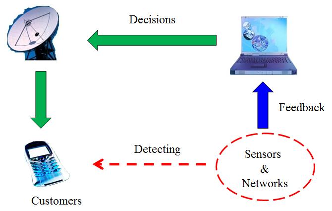
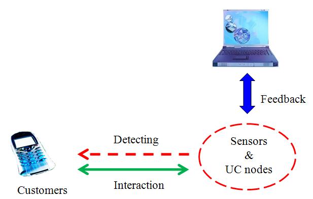
qualitatively changing in past years, utilizing the latest computer and sensor technologies. The differences between traditional and ubiquitous computing environments are shown in Fig. 2.1. A traditional computing system is known as a centralized control system, as in Fig. 2.1(a). In this kind of system, input devices like sensors, keyboards, or mouses receive instructions from or detect signals from people then pass the service requirements through the networks to the server. The central server will make decisions and relay answers or services to people. In this situation, the server has a heavy load, handling many requirements from various sensor locations. However, in the ubiquitous computing system, people only need to interact with specific UC nodes and receive the services from these nodes. The server is just an optional function in the background to monitor or learn the serving experience from UC nodes (Mostefaoui et al., 2008).

a. Traditional computing environment.

Iterature Reviews And Proposed Methodologies

b. Ubiquitous computing with immersing sensors networks. Fig. 2.1. The comparison between traditional and ubiquitous computing. The most salient features of UC include network and application scalability, wireless network connectivity, adaptability and context-aware computing,

Information

technology security and reliability and human-computer interaction (Dopico et al., 2009). The main features of UC were modified from those of virtual reality, artificial intelligence and user agent as follows (Mühlhäuher and Gurevych, 2008):

Uc Vs. Virtual Reality (Vr):

Virtual reality is an interactive environment simulated by a computer. Currently, most big computer screen for stereoscopic display or the wearing of a helmet with an onboard displayer (Dopico, 2009). In this kind of system, the computer is the centre of the world.

Iterature Reviews And Proposed Methodologies

After the computer learned more knowledge, human will finally play the role of a peripheral device in computer (Mühlhäuher and Gurevych, 2008). The concept of VR involves taking the human world into the computer. In the view of Mark Weiser, UC, conversely, takes the computer into the human world. For example, in a house, humans are the centre of the living environment, and lots of UC nodes provide different computer services to them. Mark Weiser used the term “embodied virtuality” as the opposite to common VR (Mühlhäuher and Gurevych, 2008).

In the virtual reality world of UC, a vivid 3D virtual creature is usually the incarnation of UC in such an environment. It is the highest level in a UC system to respond human’s command or pose. An example is the work of Kim et al. (2007), who developed an animated dog called Rity. Rity was shown on a computer monitor and interacted with customers. Rity was implemented on a mobile robot, but could move anywhere via internet devices as the host of an intelligent system.

Uc Vs. Artificial Intelligence (Ai):

In the past, the focus of artificial intelligence was on the methodologies for creating a machine to think and behave as a human (Russel and Peter, 2003). In the times of Mark Weiser, as sufficient realization and definition of the human brain was lacking, artificial intelligence was thought of as an unrealistic ideal (Mühlhäuher and Gurevych, 2008).

Instead of building an omnipotent computer, Mark Weiser proposed that an autonomous intelligent system should be based on limited knowledge and task, and work within a specific environment. The ultimate goal of reaching the equivalent performance of a

Iterature Reviews And Proposed Methodologies

real cognitive system would be realized by connecting every subset in UC. Thus he preferred to substitute the term intelligent with smart. That means where every UC node only took care about the limited understanding by its incoming information from individual environment. This kind of computing system is also known as the context-aware computer (Dopico et al., 2009, Mostefaoui et al., 2008).

Uc Vs. User Agents (Uas):

This was a software-based function, proposed as another intelligent function beyond AI, which was supposed to be an essential intermedium between users and computer UA was also required to be loyal to humans and learn experiences from them. In comparison with VR and AI, this function was thought of as a redundant consideration, since it overlapped with some features of AI but lacked detailed realization. As this function was denounced for over-expectation, the general concept of UC nowadays usually denotes a combination of VR and AI (Mühlhäuher and Gurevych, 2008).

From these UC features, it can be seen that Mark Weiser’s motivation was still based on the ambition to build a cognitive system. However, in spite of the ethical problems involved in humanoid AI technologies, the issue of overcoming the predicaments of cognitive intelligence development was from over capability of general-purpose computers. Therefore, in order to increase the feasibility for a modest cognitive system, Weiser attempted to distribute specific tasks into different miniature systems (embedded systems).

Ambient Intelligence (Ami)

Although Mark Weiser did not express the detail mechanisms to build a UC system (Mühlhäuher and Gurevych, 2008), UC has become an important stream in distributed computing. The most specific and successful development is nowadays recognized as The ambient intelligent system is a collection of human-centric and UC based technologies, originating from the European Commission in 2001. Utilizing the advantages of UC, the ultimate objective of AmI is to provide an information-based intelligent environment for working and living places. In such an environment, a multiplicity of embedded systems collaborates with infrastructure, portable devices, artificial intelligence technologies, wireless communication, sensing technologies and mobile agents in order to satisfy people’s living and entertainment needs (Dopico et al., 2009). Living in such intelligent environment, people would be surrounded by communication and sensor networks. The current sensor technologies such as laser range-finders, infrared transceivers, microphones, ultrasonic sensors, radio devices, radio frequency identifications (RFIDs) and digital cameras can be designed for small, reliable and low-cost perceptional features. Communication technologies such as the infrared transceiver, internet, mobile phone, Bluetooth, GPS (Global Positioning System) and Wi-Fi are utilized as the media between users and UC systems (Basten et al., 2004, Boleslaw et al., 2005).

Power consumption is another important criterion for AmI. Based on Mark Weiser’s definitions of VR, AI and UA, UC nodes can also be classified according to levels of

Iterature Reviews And Proposed Methodologies

power consumption. There are three power consumption levels in AmIs: micro-watt-nodes, milli-watt-nodes and watt-nodes. The jobs of micro-watt-nodes are gathering and transacting the data inside an embedded system, and it also possibly supplies the power for a miniature sensor. A power-supply-like solar cell could be sufficient for this kind of node. On the other hand, milli-watt-nodes work for media requiring more power, such as audio or video signals or local storage devices. The Finally, watt-nodes work like a general-purpose computer; lots of media and computation tasks deal with several local storage devices. However, the problem of watt-nodes’ computing speed usually depends on Moore’s law.

Therefore, since the UC node designs need to satisfy the requirements of portability, variance, distribution, intelligence in AmIs systems, the high power consumption of PCs is unsuitable for AmI. The novel embedded system, in contrast, is more feasible in such a system (Basten et al., 2004).

Ubiquitous Robots

For ubiquitous computing on robotic systems, called Ubibot, developments have also been based on Mark Weiser’s concepts. The Ubibot was created as a mobile platform (robot) for UC. It can spare the interfaces to communicate with a server or system operator, sensing targets or receiving requirements from people. It possesses the ability to understand the environment and to make decisions based on a specific environment, which is called being context-aware.

Iterature Reviews And Proposed Methodologies

The better definitions of a Ubibot’s structure are belonged to Kim’s job (2006), who divided his Ubibot into Mobot, Sobot and Embot. Comparing to the features of UC, the user interface of VR is called Sobot, e.g. the virtual dog Rity; it is the software-based virtual creature with the capability of interacting with people (customers) and its environment. The Sobot does not have any physical mobile ability, so it needs to collaborate with Mobot. The Mobot is a hardware-based mobile platform (robot) equipped with actuators providing physical services to customers. Meanwhile, a staff in the background monitors the robot via a graphic user interface (GUI). Finally, the sensory systems on the mobile robot are named Embot to detect the customers’ or other robots’ locations by utilizing the cameras, microphones or RFIDs underlying the floor or the gate of a path (Kim, 2006).

Having surveyed the current robotics developments with UC features, I have found that there are three successful systems working in domestic and public environments. The first example of Ubibot is the Roomba carpet cleaner (Fig. 2.2) (Tribelhorn et al., 2007).

The basic model Roomba vacuums the floor by random moving. Some more advanced models can even produce a map of the indoor environment when they bump into any obstacle. This kind of robot is also a low-cost and programmable embedded system.

Interactive ability can be enhanced by implementing extra sensors such as digital cameras, Wi-Fi and Bluetooth on top of the robots. Roomba’s vendor also provides the OS to reprogram the robot with C or C++ programming languages for various tasks as a Mobot. Re-programming ability can be achieved through the interfaces of RS232 and USB to a working station or another mini-computer installed on top of the robot (Kurt, 2007).

Iterature Reviews And Proposed Methodologies

Fig. 2.2. Vacuum cleaner Roomba. (Tribelhorn et al., 2007)

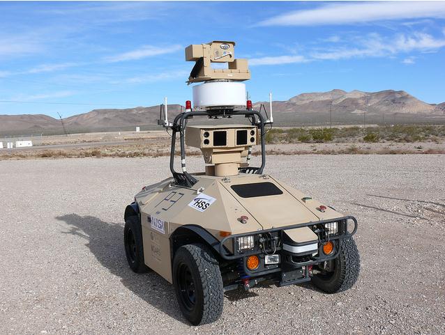
Fig. 2.3. Guarding Robot Mdars. (Nnsa, 2010)

Another well-known design is the guarding robot working in the US army. The mobile detection assessment response system (MDARS) can control mobile robots carrying wireless communication systems, GPS, sensors or even machine gun to patrol in hazardous areas, barracks, airports or the border; see Fig. 2.3. MDARS is a

Iterature Reviews And Proposed Methodologies

semi-autonomous robot system and follows the scheduled paths in field. When it detects an intruder, a warning will be sent to system operator for decision making (Holland et al., 1995, NNSA, 2010).

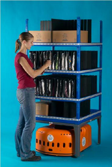
In the manufacturing industry, an inventory robotics system for warehouses called Kiva has been developed (D’Andrea, 2008), shown in Fig. 2.4. The Kiva robot is a flat, round, wheeled platform which has shelves on top and moves in the warehouse. Operators in the warehouse can command these mobile robots to pick up the inventories from specific locations via a desktop computer, then ask the robots to bring these inventories to the operators’ locations (D’Andrea et al., 2008).

Fig. 2.4. Kiva carrying things. (D’Andrea et al., 2008)

Iterature Reviews And Proposed Methodologies

Although people did not implement vivid 3D creatures on the above-mentioned robots, they were all designed with some UC features. Firstly, each robot operates around peoples’ living spaces and receives requirements from customers via various sensor technologies. Secondly, these robots were only designed with limited knowledge of their working environments. Thirdly, every remote station can provide services independently or via exchanging information from other stations. This fits in with the operations of a single UC node, node to node or node to a server.

In conclusion, when people are keen to explore the trend and necessity of a fully AI society, mobile robots within the concept of ubiquitous computing can provide hope of lessening humans’ burdens in the house, factory, or in any hazardous location. Therefore, while human-like cognitive systems are still in their infant stages, UC-based products have revealed a new commercial opportunity in the AI industry and army.

Lassification Of Ubiquitous Robots

As mentioned in the above description of research methodology and justification (Section 1.3), research focus was on exploiting novel sensor and system control technologies. In this section, various Ubibot systems are surveyed, with focus on their hardware features. These systems can be classified by different control schemes and tracking media.

Survey Of Control Schemes

Three Ubibot control schemes can be differentiated according to the location of the

Iterature Reviews And Proposed Methodologies

computing system. The first type of Ubibot system is the onboard computing robot. This kind of control design carries the whole computing system on a robot. The robot is equipped with the capability of interacting with customers and finishes specific tasks by itself (Kim, 2006). An additional feature is that the system operator can communicate with and monitor the robot via wireless communication.

The second type of Ubibot is the outboard computing robot. The intelligent control system is not embedded in the robot, and the robot has only basic control functions onboard. The outboard computer generally has no limitation on the dimension or computing ability. It can be constructed as a server tracking and controlling the robot remotely via wireless communication (Stubbs et al., 2006).

The third type is the hybrid computing system. This robot sends only complicated computing tasks to an external server. Meanwhile, this kind of robot is also equipped with some intelligent abilities, such as making the decisions for steering control and obstacle avoidance (Fierro et al., 2002).

Survey Of Tracking Media

When classifying Ubibots’ configuration by their tracking media, the relevant discussion deals with sensor technologies. The sensors for robotic tracking can also be classified as passive or active sensing devices.

Passive Sensors

The most popular passive sensor in Ubibot systems is passive wireless RFID. An RFID

Iterature Reviews And Proposed Methodologies

system is composed of tags, a reader and a host. The tags are attached to targets such as products in a shop or warehouse, and store information about the products, such as names and weights. A tag is designed with an antenna and units to process, receive and transmit information. The reader is designed to read the contents of the tag, then send them back to the host (Yan et al., 2008).

Unlike active RFID tags, which are equipped with batteries for long distance communication, passive RFID can only operate using the inductive energy of the RF (radio frequency) signals from readers. This kind of RFID, therefore, has only a short communicating distance (Zhang et al., 2010, Symonds et al., 2009). Such limited communicating distance allows people to design specific indoor environments with large RFID matrices underlying the floor. The robot can thus realize its location by reading the RFID information below the floor (Kim, 2006). Reasonable accuracy can be easily achieved by controlling the density of RFID tags.

Finally, the digital camera is another popular passive sensor. In recent years, the image quality and price of digital cameras have been significantly improved. More information, such as colours, contours and textures, can be gained from the features of image than from RFIDs (Nixon and Aguado, 2008). For example, a popular algorithm called Scale-Invariant Feature (SIFT) detection utilizes the digital camera to capture the interested image frame for feature matching (Wang et al., 2006).

Active Sensors

A disadvantage of using passive sensors is that there is less flexibility for

Iterature Reviews And Proposed Methodologies

implementation. The underlying RFID matrices involve high costs and working-hours for indoor or outdoor construction, and the digital camera usually needs to re-calibrate if the installation conditions are changed. Using active sensors seems more viable in various installations. For example, an alternative scheme to the sensing matrix under the floor is the installation of sensors on the ceiling. In such a situation, one can measure the relative distance by using active RFIDs or ultrasonic sensors to calculate the time-of-flight (TOF) between the sensors and the robot and sending the information to the host (Cho et al., 2008a). The RF signal can also cooperate with stationary or mobile landmarks. In a similar way to the mechanism of TOF, the location of a robot can be measured by comparing the arrival time of the RF signal to each landmark in the sensing matrix. From the same radio system, the distances between the robot and the landmarks are roughly estimated by the RF received signal strength (RSS), which is a function related to the distances between a robot and landmarks (Chen, 2006).

a satellite-based matrices laid out on the orbit. The orbital matrix is normally divided into six regions, and every region contains four satellites. This arrangement guarantees that any location on the earth can face four to ten satellites. Only four satellites, however, are sufficient to provide information about a target’s position and speed (Ahmed, 2002). Currently, a low-cost GPS system can provide reasonable accuracy, with an error within 5 metres (Tessier et al., 2006). This feature is very useful in outdoor environments. Unfortunately, GPS signals are easily shielded in indoor environments.

Besides ultra-sonic and RF signals, laser is another popular medium using TOF for

Iterature Reviews And Proposed Methodologies

distance detection. A product called the laser scanner can scan and measure the distance between a robot and surrounding obstacles, compare with an inbound map or create a new map in real-time (Chung et al, 2006). However, laser signals are easily reflected by mirrors, rain and fog.

When a digital camera is combined with lasers for TOF distance measurement, a digital camera which is an active sensor is produced. This kind of camera is equipped with many laser LEDs (Light Emitting Diodes) illuminating the target. The reflection of the laser is captured by the camera. The image produced by the camera is displayed in specific colours that represent in depth to the target (Dubois and Hüglí, 2007).

Overview

Digital logic circuit designs on chip are generally based on standard large-scale integrated (LSI) modules, such as the microprocessor or system clock generator. Sometimes, as a complete system, there are still additional logic functions (call glue functions) which need to be integrated into the chip in order to reduce the complexity of printed circuit board (PCB) layout (Deschamps et al., 2006). This kind of extra requirement can be solved by ordering a custom integrated chip. Custom integrated circuits are classified as full-custom and semi-custom application-specific integrated circuits (ASICs) (John, 1997). However, developing a custom chip is quite expensive.

Iterature Reviews And Proposed Methodologies

Hence, in 1984, XilinxTM first introduced the hardware-programmable device FPGA as an alternative low-cost scheme. This allows a customer to implement the glue functions on a chip by programming (Deschamps et al., 2006).

Fpga Architecture

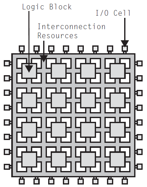
In comparison with ASICs, FPGAs have fewer choices for circuitry optimization. In fact, the FPGA is only similar to the gate array category in ASICs (Zeidman, 2007). The inside of an FPGA is regularly laid out with configurable logic blocks, I/O blocks and interconnections, as shown in Fig. 2.5. New generations of FPGAs might also include embedded memory, microprocessors, hardware multipliers and phase-locked loops (PLLs) circuits (Dueby, 2009), called Macro cell in Xilinx (Chu, 2008).

Onfigurable Logic Blocks

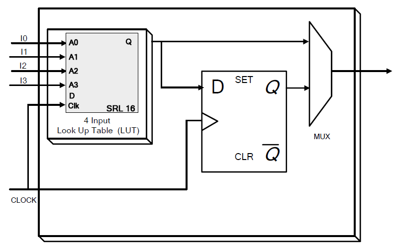
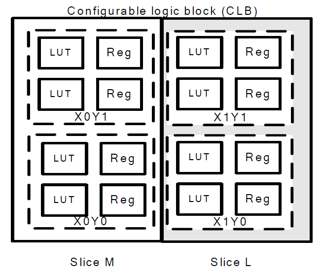
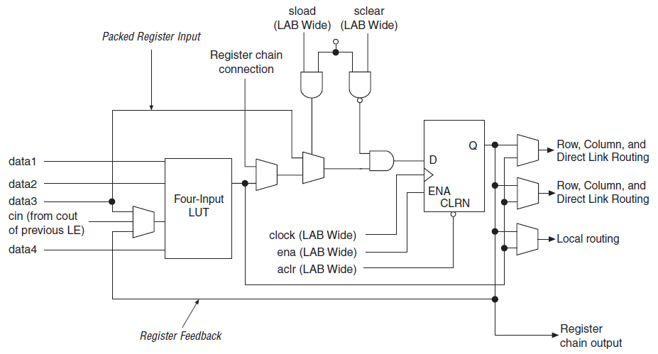
Configurable logic blocks are designed with the programmable logic of FPGA. Every block can be subdivided into basic logic units called logic cells (LCs) in Xilinx. Nowadays, a basic logic cell is usually a memory RAM (random-access memory) based look-up table (LUT). It can be thought as an n-input and one output memory storing desired gate logic as shown in Fig. 2.6(a). Logic cells also contain carry circuits for arithmetic functions and output multiplexor circuits. Two to six LCs comprise a larger unit called a slice in Xilinx’s latest FPGA, and two to four slices comprise a big block, which is the configurable logic block (CLB), for higher flexibility and performance reasons (Chu, 2008, Dueby, 2009), as in Fig. 2.6(b).

Iterature Reviews And Proposed Methodologies

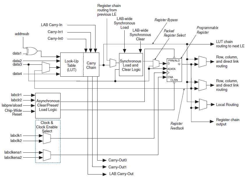
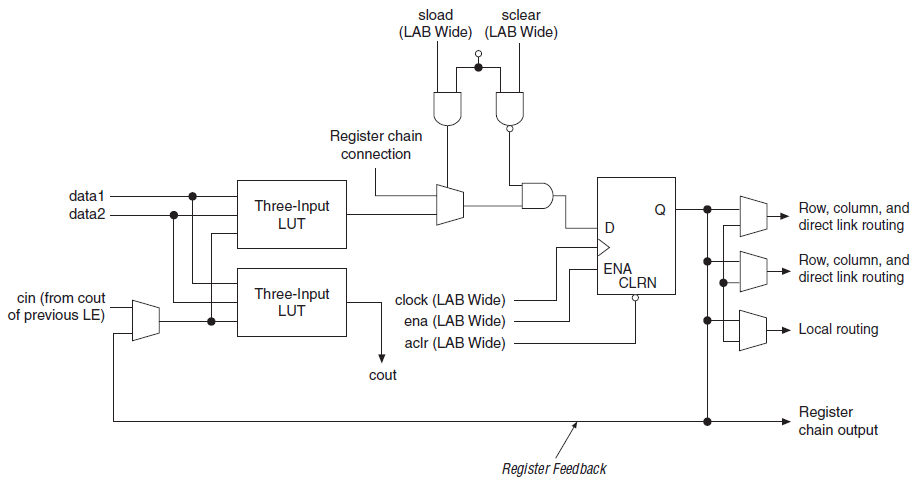
b. CLB block consisted by LCs. Fig. 2.6. Structure of a CLB block on Xilinx SPARTAN-3. (Dueby, 2009) Similarly, Altera’s basic logic unit is called a logic element (LE), as in Fig. 2.7(a). Every LE in the Cyclone II also contains a four input LUT. Sixteen LEs directly comprise a big logic array block (LAB) in Cyclone II. The register chain input signal shown in Fig.

2.7(a) can cascade the LUTs in the same LAB together to perform a combinational function or shift register. There are two operating modes in LE, named normal and arithmetic modes. The LE under the normal mode is designed to perform the general logic applications and combinational functions (see Fig. 2.7(b)). When the LE is under the arithmetic mode, the LE becomes a 2-bit full adder with carry chain function, as in Figs. 2.7(a) and (c). The arithmetic mode is designed for the adders, counters, accumulators, or comparators (Altera, 2007).

Iterature Reviews And Proposed Methodologies

a. Structure of a LE. b. LE in a normal mode.

Iterature Reviews And Proposed Methodologies

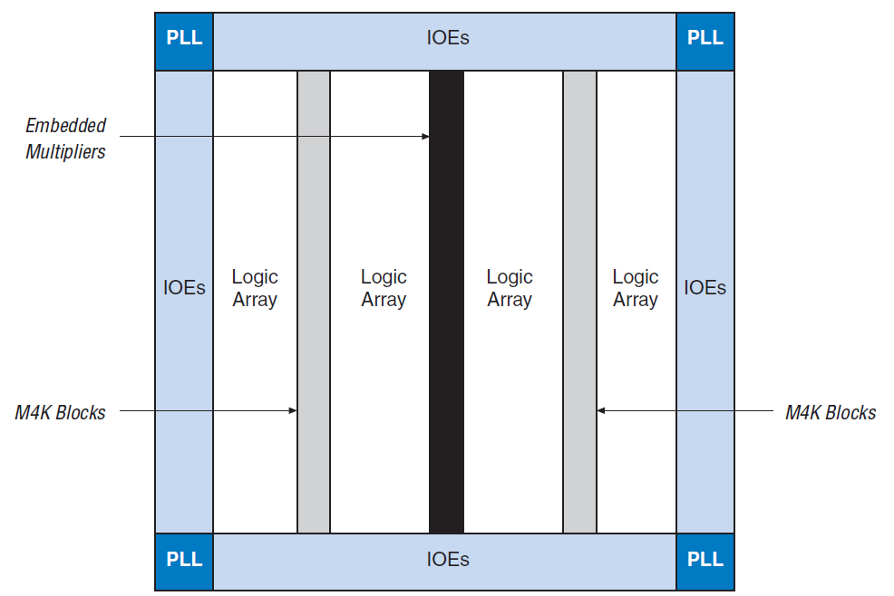
c. LE in an arithmetic mode. d. Cyclone II EP2C20 block diagram. Fig. 2.7. Architecture of Altera Cyclone II. (Altera, 2007)

Iterature Reviews And Proposed Methodologies

Finally, the block diagram of a Cyclone II EP2C20 FPGA is shown in Fig. 2.7(d) as an example. The LABs in FPGA are mainly divided into four blocks, and one block of multipliers is located at the middle of FPGA, which can directly connect to adjacent LABs or via row/column interconnections. Two M4K blocks are the embedded memory RAM where every sub-block in this area contains 4k-bit memory space with operating speeds up to 260MHz. In addition, the Cyclone II also includes four PLLs which can be utilized as a high speed system clock generator (Altera, 2007).

Fpga-Interconnection

The interconnections in a FPGA is consisted with direct-link (or short line) and programmable switches (Zeidman, 2007). Direct-link allows a logic block, e.g. CLB or LAB, directly connecting to its neighbouring blocks (Altera, 2007, Zeidman, 2007).

When a logic block needs to communicate with another block at long location, it will need various traces in row and column directions to route the signal. The row and column traces are passing by different blocks. The connection and routing mechanism, therefore, depend on the programmable switches (Chu, 2008, Zeidman, 2007).

The programmable switches of FPGAs are based on three technologies: static RAM (SRAM), erasable flash-based and anti-fuse (Dueby, 2009) interconnection switches. These technologies are also correlative to FPGAs’ programmable logic structures.

SRAM interconnection switches are currently main-stream in Altera and Xilinx. SRAM is a volatile component and will lose configuration after power is turned off, so this kind of device usually needs external memory to store the configuration of connections.

Meanwhile, these devices also have a higher static power consumption to maintain their

Iterature Reviews And Proposed Methodologies

configuration (Dueby, 2009). The advantages are that SRAM-based FPGAs have the features in easy reprograming and including low cost memory (Zeidman, 2007). Contrary to SRAM, the non-volatile flash-based memory can keep interconnection configuration after power is removed, and the static power consumption is much less than in the SRAM structure (Dueby, 2009). The structure of flash-based FPGAs is basically the same as the SRAM-based FPGAs except the different reprogramming mechanism (Zeidman, 2007).

The anti-fuse method programs gate arrays in a similar way to blowing a fuse. In the initial state, the fuse is a link between two conductors (traces). Once a large voltage is applied across the link, the link melts and leads both conductors migrate across the link to create conducting. Although interconnection programming with such a method is permanent and less flexible, the anti-fuse based FPGAs have the advantage of avoiding interferences from radiation and power glitches, and they are also faster than SRAM (Zeidman, 2007).

Finally, since the interconnection of latest FPGAs are designed with SRAM components, the signal propagating speed is much slower than in ASICs, in which signals are routed in metal layers, leading to pure RC delay (Zeidman, 2007).

Onfigurable I/O Block

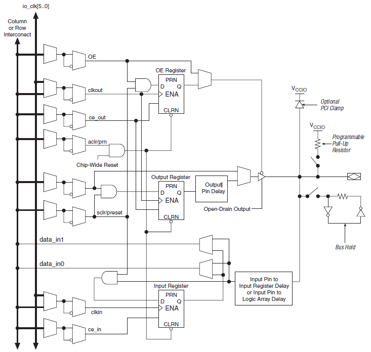
The configurable I/O block is the buffer between the logic blocks and external devices. Fig. 2.8 shows an example of the configurable I/O circuits of Cyclone II, the IOE (I/O

Iterature Reviews And Proposed Methodologies

element), where the interface supports differential and single-ended signals. The differential signal consists of two single-ended ports with inverted signals. Additional reconfigurable pull-up resistor is designed for every single open-drain output signal. An IOE consists of three registers for bi-directional communication, named as the input, output and OE registers. The input register is only synchronous with the system I/O clock for fast setup time, but the output register has the additional choice to hold output signal by an enable signal from OE (output enable) register (Altera, 2007).

Fig. 2.8. Configurable IOE on Cyclone II. (Altera, 2007)

Fpgas In Robotic Design

An attractive feature of the FPGA is its omnipotent capability in digital circuit designs. From the basic RTL level, it can be utilized for the automation control. For example, in a smart car system, a braking nervous factor (BNF) is proposed to predict the braking responses of a driver for arbitrary values of the safe stop distance to the front vehicle and relative speed of the two vehicles moving in a straight line. The proposed RTL-based SOPC and BNF control system can also learn the braking behavior of the driver to create an experience database for the autonomous driving mode (Yu et al., 2008).

Besides, FPGA is the interface between a microprocessor and peripheral sensors (Xu et al., 2008). One of the resultant applications is translating image data from digital cameras into the instruction format of a microprocessor. Meanwhile, object tracking with digital cameras can also be achieved by classifying specific colours on objects or using particle filter methodology (Meng et al., 2007, Zhou et al., 2005, Cho, 2007).

For mathematics, FPGA is the favoured choice for real-time computation (rather than microprocessors). By implementing the differential and integral operations as a PID (proportional-integral-derivative) controller, one can achieve a motor control system (Kim, 2007b). Common arithmetic such as trigonometric functions with floating point numbers in hardware circuits is faster than in a microprocessor (Kurian, 2009, Detrey and Dinechin, 2007).

In addition, FPGA can also realize low-cost DSPs (digital signal processors) for signal

Iterature Reviews And Proposed Methodologies

processing such as digital signal filters (Kilts, 2007). Some FPGA vendors even provide the IPs for low-end microprocessors which allow users to run the OS with C programming language. Users can directly implement the whole system on a single FPGA chip without cooperating with extra microprocessors (Chakravarthy and Xiao, 2006, Dueby, 2009).

Proposed Approaches

Having examined the above approaches to robotic control scheme designs, sensor outboard computing model for multiple robot formation control. This strategy was inspired by the work of Stubbs (Stubbs et al., 2006). A global digital camera with an FPGA platform for surveillance and robot control as built.

The consideration of an outboard scheme was based on the limited battery power capacity and computing ability of a mobile robot, which leaded difficulties using onboard computing system. A high power consumption system not only reduces robot’s operating duration, but also reduces battery life by frequent recharging. Secondly, although a microprocessor with a low system clock consumes less power, low computing abilities might have significant delay with complicated tasks. Thirdly, using the hybrid computing model to send computed data to the robot via wireless communication might face limited data throughput and security issues. Consequently, research was focused on the methodologies for developing a power-efficient and integrated computing node, which could guide deployed robots without extra modification of the robot or of the indoor environment. Here the microprocessor on the

Iterature Reviews And Proposed Methodologies

robot was only dealing with mechanical steering. All tactical decisions and robotic tracking were performed on an external FPGA platform. For the detection abilities, a digital camera was to be utilized as the global passive sensor with an outboard computing system. The different information for control algorithms was expected to be attained from a single camera. Thus reduced the hardware cost without installing various sensors. Besides, the passive sensors also have the advantage of operating without disturbance between robots within crowded active sensor networks. Moreover, not possessing the active detecting components found in a laser range finder or TOF camera, the low-end digital camera generally consumes less power. Finally, based on price, the infrared signal was temporarily adopted for wireless communication with the robots.

To reach a low-cost detection system with digital image, the FPGA obtained all the critical information from a monocular digital camera. This camera worked as a global camera tracking the robots by their circular identification (label) on their tops via the colour discrimination algorithm. Each robot’s label was designated with the same colours. Thus, every robot had to start off its manoeuvre from a specified docking area.

In this docking area, the FPGA locked the label by the specific colour and tracked it around the working area. Unlike the dual or multiple colours designs described by Liang et al. (2008), Stubbs et al. (2006) and Riggs et al. (2010), this arrangement mitigates the burden of recognizing various colours on multiple robots. By discriminating the feature of dynamic colour pixels on serial pictures, a real-time motion detection using the one-page-comparison (OPC) algorithm and inbound memory of FPGA was proposed for security function.

Iterature Reviews And Proposed Methodologies

Without the detection algorithms with the TOF mechanism, a method to estimate the inter-distance of a robot group was proposed, which was also to be derived from a digital camera. The difference is that the algorithm does not utilize any homography or camera calibration procedures due to their complication. The proposed algorithm allows a user to directly install with the generic camera by lacking the information about focal length of the lens, installation height and tilting angles. The required information of estimation is only the dimensions of robots’ circular label. In the following chapter, it will demonstrate the satisfactory accuracy and real-time performance for relative distance estimation.

Finally, since a monocular camera can derive relative distance between robots, the trajectory tangent of a robot can also be derived by a similar method. A trajectory generation design can measure a robot’s 2D orientation and movement by integrating the instant moving distance. Using behaviour-based steering such as left turn (L), right turn (R) and straight drive, the complicated kinematics of low-speed mobile robots on a 2D plane can be simply replaced by the calculation of the trajectory tangent, called slope in mathematics. These algorithms realized a real-time multi-robot formation control without any complicated functions or operations but with comparable performance in computing speed and energy efficiency.

System Architecture And Devices

This chapter provides a comprehensive introduction to system architecture, devices and FPGA design tools. In Section 3.1, a description of robotic formation control schemes and chip functions is provided. The leading role of the Cyclone II FPGA developing platform is introduced in Section 3.2. The specification of the digital camera module follows in the next section. In Sections 3.4 and 3.5, the configuration of the miniature robot Eyebot and remote mechanism are detailed. Introductions to the hardware description language and design tools for FPGA are contained in the last section.

System Architecture

Fig. 3.1(a) depicts the operating scheme of the proposed Ubibot system. In this prototype, a monocular digital camera is installed as the global camera, facing the floor. The picture quality is set to 1280  1024 pixels and 34 fps frame rate. A low-power FPGA chip plays the role of an outboard server for image processing, object tracking and multiple robot formation control. Control signals are transmitted to the robots via infrared. With this blueprint, the FPGA aims to perform a basic three robot formation with Eyebots.

Once the FPGA receives the commands to track the robots and to perform formation

System Architecture And Devices

driving, the closed loop feedback control starts from the input images of the digital camera. Here, the FPGA tracks objects with the ability to tilt and pan the camera for a larger monitoring area. To initialize the tracking mechanism, every Eyebot needs firstly to pass through a docking area designated on the monitor. The FPGA can thereafter track the labels attached to the top of the robots. During the driving procedures, a window of interest follows every label at all times. After the FPGA derives the tracking and steering strategies, it transmits the guiding signals to the robots via an infrared spotlight for a wide range remote control.

The proposed image-processing and formation control mechanisms are all integrated into a single FPGA chip. Fig. 3.1(b) is a systematized function diagram of the FPGA chip. There are three group designs in FPGA handling tracking and steering abilities.

These three group data paths in the chip work in parallel and individually, where each group in the chip is assigned to control an Eyebot. Such architecture is also classified as the decentralized control in the chip.

The system installation and real-life image on the monitor are shown in Fig. 3.2, where an FPGA developing platform cooperates with an infrared spotlight on the top, a computer monitor and three Eyebots on the floor. With the arrangement in Fig. 3.1(b), all functions are intended to be designed with RTL or gate level circuits in order to reach the real-time requirement. Whole algorithms are directly transferred from high-level programming logic into lower level circuits. Thus no external memory device is required to save the program for operations. The only external memory used here is for buffering the image data for the VGA interface. Captured images shown on the monitor represent surveillance function to a system supervisor. Finally, by comparing

System Architecture And Devices

the dynamic pixel of sequential images, an extra security design cooperating with the digital camera is also integrated into the FPGA chip as the motion detection in Fig. 3.1(b).

Based on the concept of Ubibot, the chip design of the FPGA realizes node computing as a reconfigurable embedded system. The surveillance function is represented by the image on monitor. Context-aware computing is achieved for multiple robot formation driving by the knowledge of colour discrimination and relative distance estimation.

(a) Formation of multiple robots.

System Architecture And Devices

(b) Functions of chip designs. Fig. 3.1. Multiple robot formation control scheme with chip design. 3.2. Whole system installation.

Fpga Developing Platform

The Altera DE2-70 developing platform is designed with a low-power Cyclone II FPGA, EP2C70F896C6. It is produced using the 90nm transistor process and has a maximal power consumption of about 3.9W when running at 150MHz and 85℃ (worst case). A comparison of the Cyclone II family features is shown in Table 3.1 (Altera, 2007).

Table 3.1. Cyclone II family features. (Altera, 2007) The EP2C70 is the biggest FPGA of the Cyclone II family. It is designed with 68,416 LEs and inbound 1.152M bits RAM. Four PLLs blocks can be utilized to generate a high speed clock for VGA and external memory SDRAM (Synchronous Dynamic Random Access Memory). The maximum operating speed of the Cyclone II is up to 260 MHz, so it can support the low-speed memory modules of DDR (double data rate) or DDR2, the common interface PCI (Peripheral Component Interconnect) or PCI Express interface (Altera, 2007). However, although the EP2C70 can support some high speed

System Architecture And Devices

devices, the highest system clock is still much lower than current PCs. The DE2-70 developing platform is produced by Terasic. It is a versatile developing platform and used in many top universities as an educational kit for digital and microprocessor design courses. The advantage of this FPGA developing platform stems from various peripheral interfaces of current computer systems, such as USB (Universal Serial Bus), RS-232 serial port, VGA, Ethernet, audio, IDE (Integrated Device Electronics), video, TV, SD memory card and infrared transceiver. These interfaces provide a suitable environment for helping designers to implement communication between UC systems and PCs. In spite of the support for various interfaces, another attractive feature of the Cyclone II FPGA is the capability for low-end microprocessor design. The standard IP for the general-purpose microprocessor Nios II is provided by Altera. The user can directly implement Nios II on FPGA and program with C language.

For signal processing, the Altera IP also provides low-cost DSP for users with Mathworks Simulink and Matlab design environments (Altera, 2007). An outline of the DE2-70 platform is shown in Fig. 3.3 (Terasic, 2007). Two 32M bytes SDRAM are working as the image buffer for the VGA interface. One on-board LCD (Liquid Crystal Display) module is for reading the data of the FPGA. Eighteen toggle switches are used to designate the initial state of the system. Four push-buttons provide the triggers to initialize the tracking and formation procedures. The camera frame rate is shown on the 7-segment displays in hexadecimal readings. Designer’s circuits can be downloaded from the USB blaster port 1. The RS-232 port is reconfigured for the image input.

System Architecture And Devices

Fig. 3.3. DE2-70 FPGA developing platform. (Terasic, 2007)

Igital Camera Module

Using CCDs (Charge Coupled Devices) and CMOS (Complementary Metal Oxide Silicon) based components is main-stream in modern digital cameras. Both image sensors are designed with the array structure. Resolution of an image is decided by the number of image sensors (pixels) on an array. The pixels of a CCD camera accumulate charge proportional to the incident light strength, which is then transferred into digital signals. On the other hand, CMOS cameras contain several transistors on every pixel to amplify the incident light signal (Nixon and Aguado, 2008). Recently, CMOS cameras have significantly improved in noise. Having the advantages of lower power consumption, smaller pixel dimension, low-cost and high frame rate, CMOS digital sensor modules have been developed for mobile phones, PDAs, toys and other battery-powered products (Micron, 2004).

In the proposed Ubibot system, the adopted digital camera module TRDB-D5M is also produced by Terasic, as in Fig. 3.4. It is a low-cost, high resolution and high frame rate CMOS camera module. This module provides a wide range of image qualities for designers. The various choices for frame rate and resolution can be seen in Table 3.2 (Terasic, 2008). The digital shutter speed (frame rate) of camera is decided by the exposure time of pixels. Low shutter speed will degrade the performance of real-time object tracking. Here the digital camera in my Ubibot system is set for SXGA standard with 1.3M pixels resolution and 34 fps frame rate for better image quality and tracking performance.

System Architecture And Devices

Fig. 3.4. TRDB-D5M digital camera module. Table 3.2. Different operating modes of TRDB-D5M digital camera module. (Terasic,

Obile Robot Eyebot

The mobile Eyebot, also known as the differential drive robot, is a two wheel battery-powered miniature robot as shown in Fig. 3.5(a) (Bräunl, 2006). The software programming based embedded system comes equipped with a 25MHz/32bit microprocessor (Motorola M68332) and 1-2MB of external RAM. 512KB of read-only memory (ROM) is used for storing the basic input/output system (BIOS) of the Eyebot or for downloading the driving programs from a computer. In this project, the driving program was programmed with C language, and the instruction library was provided by the system vendor.

The name Eyebot originates from its frontal digital camera of 60  80 pixels resolution. The object detected by the camera is shown on a grey-coloured LCD monitor on the top of the Eyebot with 64  128 pixels resolution. Operating conditions such as downloaded programs, functional menu and system conditions can also be read from this LCD monitor; see Fig. 3.5(b). However, due to the robot formation system being designed with the outboard computing system, the digital camera on the Eyebot was not used in this project.

Some important interfaces are also shown in Fig. 3.5(b). The IR receiver in the top-right-hand corner receives an infrared signal with TV remote codes. The infrared signal is from the FPGA platform, transmitted by an infrared spot light. Actually, the Eyebot system only provides 35 buttons (instructions) from a TV controller for robotic control. Serial 1 allows user to download the programs through a RS-232 interface. Four input buttons are used to select the system functions and to set the start of the driving

System Architecture And Devices

a. Side view of Eyebot. b. Interfaces of Eyebot (Bräunl, 2006). Fig. 3.5. The Eyebot.

System Architecture And Devices

For driving control on the robot side, the Eyebot’s two wheels are driven by individual motors as the differential driving. When the user assigns a specific driving speed, the Eyebot’s instruction library automatically links the PI (Proportional, Integral) controller to track the desired driving velocity, orientation and distance, as shown in Fig. 3.7.

Fig. 3.7. Driving control scheme of Eyebot. (Bräunl, 2006) Finally, in this project, there was little effort involved in programming the Eyebots, because the driving decisions were designed and integrated in the FPGA chip. The programs on the Eyebot only deal with constrained driving abilities, e.g. driving forward or turning.

Wireless Remote Signal

A low-cost infrared system was adopted for one-way wireless control. The remote instructions are from the SP-URC-81 TV controller provided with the Eyebot system. Without hacking the instruction library of the Eyebot, here the original infrared instruction sets are kept for wireless communication.

Fig. 3.8 illustrates the real waveform structure of the SP-URC-81 TV remote code on

System Architecture And Devices

the oscilloscope with button “0”. It can be seen that the infrared signal combines with modulation and Manchester encoding in 16 bits format. The modulation mechanism was with 37 kHz pulses, as in Fig. 3.8(a). Based on the modulation pulses, a 432ms interval represents a digital bit; see Figs. 3.8(b) and (c). Finally, the remote instruction consists The Manchester encoding is utilized to represent the different instructions for driving control and data. This is translated in Hexadecimal in Eyebot’s instruction library (see Appendices A and B). However, unlike the formal bi-phase Manchester encoding, the battery-powered system only has the physical transition from 0V to positive voltages.

Thus the logic “1” in the Eyebot is confirmed when the digital signal transits from 0V to positive voltages, and the signal transiting from positive voltages to 0V is for logic “0”. Total SP-URC-81 TV remote codes of the Eyebot are shown in the Table A.1 of Appendix A. One TV button (instruction) only represents single behaviour or data.

Therefore, without hacking the Eyebot’s instruction library, there are only totally 35 activities or data sets can be used in this Ubibot system.

Fpga Development Kits

Contrary to the digital system design by drawing schematics, a complicated digital circuit can be conveniently programmed by hardware description language (HDL). In this project, two of the most widely used hardware description languages, VHDL and Verilog, were adopted alternately. Both languages were developed as industry standards for digital hardware modeling and synthesizing for programmable devices such as FPGAs, complex programmable logic devices (CPLDs) and ASICs. The FPGA and

System Architecture And Devices

CPLD devices are mostly reconfigurable logic devices, while ASIC has fixed customized-function (Pedroni, 2004). VHDL is the acronym for VHSIC (Very High Speed Integrated Circuit) hardware description language (Hwang, 2005). It was initially funded by the United States developed by the CAD (Computer-Aided Design) vendor Gateway in the 1980s and difference between two languages is that VHDL is based on the syntax of ADA and PASCAL programming language, and Verilog is based on the C programming syntax (Hamblen et al., 2006). A brief introduction to VHDL and Verilog programming structures has been laid out in Appendix D.

Both hardware description languages for FPGA designs are working with the Quartus II software from Altera. Similar to the other professional CAD tools, Quartus II is a CAD tool to design the programmable FPGA, CPLD and ASIC products of Altera. It allows a user to design digital circuits (modules) via HDL or by drawing real gate circuits. It provides services such as synthesis, initial thermal estimation, circuits in RTL module, generation of the finite state diagrams, calculation of LE resource usage, simple timing waveform analysis and downloading of designs to devices. For simple digital circuit design, the timing waveform simulation result can be directly attained without cooperating with third party software. Detailed steps for starting off a new project and design with Quartus II are contained in Appendix E.

System Architecture And Devices

In this project, some of the basic interface modules were authorized and modified from the intellectual property (IP) of Altera and Terasic for academic purposes only. These interfaces included capturing images from a digital camera module, VGA interface and data path controller for external SDRAM memory chips.

(a) 37kHz modulation signal. (b) A basic digital bit width.

System Architecture And Devices

(c) Bits structure of button “0”. Fig. 3.8. TV remote code “0” with modulation and Manchester encoding.

Tracking

Digital cameras are popular candidates for devices employed in visual sensing applications. Their attractive features, including wide detection ranges, high resolution and reliable performance, have made them indispensable sensors in surveillance and robotic sensing. A simple way to achieve this is to capture images with a digital camera and then use algorithms to determine the different colours in each image. In this chapter, two real-time object tracking designs using an FPGA are proposed. The first design is colour discrimination (detection) which was developed to track a robot’s label (identification). This approach has the disadvantage of being constantly affected by issues such as light reflection and shadows on the object's surface. Although some sensory methodologies for colour detection are available, they are not necessarily good choices for ubiquitous robotic systems, where real-time computation ability and low power consumption are of the utmost importance. Overly complicated image processing techniques will cause some practical problems when implemented in an embedded system. The second design is motion detection prepared as a security function of the system. The proposed one-page-comparison (OPC) mechanism contributes to the

Olour Based Real-Time Object Tracking

reduction of the memory and logic gates used in an FPGA chip. By utilizing the proposed approach implemented in circuit designs, real-time colour discrimination and motion detection can be achieved with good performance, as demonstrated in this chapter.

Olour Discrimination Review

Ubiquitous robots serve as a good demonstrator for a UC society. A mobile platform carrying multi-sensory functions and intelligent information can respond to different clients in a broader navigational range than the stationary server system (Kim, 2006).

However, in contrast, a Ubibot has more critical requirements to be satisfied in a battery-powered system than the stationary computer. A solution to the limited power capacity problem has become the first priority before sensory devices and computing units can be designed (Basten et al., 2004).

One of the most important applications of sensory technologies is for robotic localization. Currently, robotic localization can be achieved by different sensors such as encoders, infrared transceivers (Cho et al., 2008b), ultrasonic sensors (Lee et al., 2008), wireless networks (Wen et al., 2007) and laser range finders (Trawny et al., 2007).

However, their performance may not always be satisfactory. For example, quadrature encoders may lose accuracy due to wheel slippage. Active sensing with infrared, ultrasonic, laser and radio signals may suffer from interference. In addition, every sensor can only provide limited environmental information based on the physical

Olour Based Real-Time Object Tracking

phenomena being measured. Therefore, a mobile platform needs to be equipped with sensors of different types. In addition to active communication strategies, passive identification is also proposed with the use of wireless RFID tags (Kim, 2006). The identifying sensor can be installed on the equipment, gate or engraved in the floor.

Compared to the aforementioned sensory technologies, the digital camera seems to have more versatile abilities with passive detection. For instance, a designated object can be tracked by identifying its contour or colour (Nixon and Aguado, 2008), the distance between camera and object can be derived by the extrinsic and intrinsic parameters of a camera system (Hartley and Zisserman, 2003), and moving objects can be detected from information gathered by surveillance video streams (Huang et al., 2008). Recently, the time-of-flight (TOF) principle has been applied to digital cameras for short-distance measurement (Rapp, 2007). The TOF camera system measures the flight time of a laser beam between the camera and objects then presents the image in a depth map with different colours. This kind of device realizes the possibility of obtaining distance information by using a monocular camera. Unfortunately, image processing with a digital camera often consumes a lot of computing effort. Thus, unless the computing speed is dramatically increased, e.g. by improving the clock speed, a significant delay will occur with increasing picture resolution and frame rate.

During the past few years, there have been promising developments for fast image processing in automation. Portable cameras can be installed to read the path information from barcodes positioned on the floor, allowing Kiva robots to instantly derive their location (if the barcodes are accurately observed) (D’Andrea and Wurman, 2008).

Alternatively, image processing on embedded robots can be achieved with an external

Olour Based Real-Time Object Tracking

server via unobstructed wireless networks. The external computer processes image data and then sends back tactical decisions to the robot (Fierro et al, 2002). More feasible models can be found in Stubbs et al. (2006) and Riggs et al. (2010), wherein the inboard camera is replaced by an array of overhead cameras, mounted on the ceiling. These cameras track coloured markers on top of each robot in a group. However, inconveniences may arise from the building fixture and calibration of the camera array.

Surveying the robot vision subsystem above, colour discrimination is the most essential perception ability. This is useful not only in helping a robot to recognize the objects by a specific colour but also in assisting the central surveillance system to track robots by their colour labels (Stubbs et al., 2006, Riggs et al., 2010). The challenges in tracking objects by their colour arise from different interferences from reflection and shadow which lead to non-ideal image representations. Reflection can be described by the physical phenomena of diffuse and specular reflection. Diffuse reflection occurs when light rays penetrating an object's surface are reflected in multiple directions, and specular reflection is known as the mirror-like reflection on the surface (Ren and Wang, 2008). Shadow can also be classified into self and cast shadows. A self-shadow is the shadow attached to the object's body that is not illuminated, while a cast shadow is projected by the object onto the ground or other objects (Salvador et al., 2001).

Consequently, in real-world practice, the colour discrimination function becomes a complicated task by the occurrence of various surface colours with interferences. A survey of the literature on reflection and shadow removing technologies reveals that the earliest reflection removing methodology can be traced back to Shafer (1985). The work details the use of the dichromatic reflection model to separate spectral properties.

Olour Based Real-Time Object Tracking

An improved methodology with photometric linearization applied to remove the reflection from a smooth metallic surface can be found in the work of Ren and Wang (2008). The other methodologies for removing reflection and shadow images include comparing different statistic measures of edges between shadow and reflection (Tappen et al., 2002), mitigating overlapped edges inside the reflection image via edge detection and comparing templates in a database (Levin et al., 2004), extracting reflection and shadow from a sequence of moving pictures (Szeliksi et al., 2000), or using a polarizing filter with kernel independent component analysis (KICA) to reduce reflection (Yamazaki et al., 2006). These complicated methodologies are based on analysis of stationary pictures on a computer monitor that may not meet the real-time requirements for a mobile ubiquitous robotic system unless the embedded system's processing speed is tremendously increased.

When robotic vision is incorporated into a cooperative control framework, the performance of the overall system will rely critically on a high-speed digital camera and the subsequent image processing procedure. However, high-speed image processing uses large amounts of power and so a feasible and effective algorithm is proposed to perform the real-time colour discrimination functions with hardware circuit designs using an FPGA. Here the colour discrimination quality is enhanced using an additional tuning parameter, implemented for dynamic adjustment of boundaries with light reflection and shadows. After the specific colour is discriminated by the FPGA, an object tracking mechanism using the window of interest can be realized by tracking the threshold of pixel numbers.

Otion Detection Review

Motion detection is one of the challenges that demands modern methodologies in machine vision. Solutions to this problem provide not only an early alarm in security design with digital image sensors is based on the image comparison method (Jing et al., 2005). The computer system receives an image from a CCD or CMOS camera module (Jáhne, 2005) and then compares subsequent images in a video stream. The variant parts of images contain dynamic scene information and can be extracted from the static background as a moving object (Nixon and Aguado, 2002).

When a motion event has occurred, the search for effective ways to express and interpret the moving object is another important issue. By using modern image processing methodologies, the moving object can be presented by different textures. In the work of Wu et al. (2004), the basic shape of a moving object is presented by a grey level image whereby the static background might be simply defined as the black area.

Other popular algorithms usually subtract the moving object directly from its static background (Yang et al., 2007) or present the moving object by extracting and illustrating its edge (Tsai and Chiu, 2008). An efficiently realizable method to identify a moving object is to assign a mark directly on the moving image (Daniels et al., 2007).

This type of design can help the user to assess the detection performance quickly without a lot of modifications from the original image. A similar marking concept can also combine with a tracking algorithm to localize the moving target within a square frame (Huang et al., 2007, McErlen, 2006).

Olour Based Real-Time Object Tracking

Although motion detection using modern image processing gives a satisfactory result, most of the algorithms used still rely on software programs running in traditional sequential computing architecture. Consequently, even for the simplest motion detection scheme, the requirements for large memory space and fast computation speed cannot be easily satisfied. Moreover, the need for high image resolution and frame rate has imposed further demands for efficient motion detectors. The difficulties with traditional computing for the detection system design are not only inefficient but also impose severe constraints for developing systems using a miniature sensor such as those employed for robot vision with a battery power supply (Tuan et al., 2007, Bräunl, 2006).

To solve the dilemmas of real-time processing, the common but undesirable solution remains a compromise with a lower resolution camera in order to reduce the computation time.

Furthermore, power consumption is another serious issue in miniature sensor applications. Some design examples, i.e. the one-bit algorithm (Lee et al., 2004), have been developed to mitigate the drawback of power limitation. The one-bit motion detection system detects motion using a reduced pixel algorithm. When the moving object does not appear in front of the camera, the motion detection system will be kept in standby mode until any moving object is detected again. However, this algorithm is also subject to defects associated with unreliable detection due to lower image resolution when in standby mode. Moreover, large power consumption is still unavoidable when tracking a moving object in normal operations.

Taking into account energy efficiency and the design challenges in a miniature motion detection system, a refined hardware circuit-based design, which aims to perform

Olour Based Real-Time Object Tracking

motion detection, could be an attractive alternative. Here, this moving object detection system considers the balance for processing delay, image resolution, low power consumption and a reduced computation complexity. These advantageous features have been verified in a prototype and simulated on an FPGA chip (Yu et al., 2009c). The proposed motion detection system using the one-page-comparison (OPC) technique is shown to be comparable to traditional motion detection designs.

4.2 Capturing images from the digital sensing array The digital camera is an image sensing device composed of a number of photo-sensitive elements (e.g. photodiodes). With embedded colour filters on top, every element on the digital image sensor array only detects a monochromatic colour in red (R), green (G), or blue (B). The output strength of each element is then transformed into digital data, in pixels, by an analog-to-digital converter (ADC) inside the camera module. The digital image sensor array in the adopted camera module is arranged in a Bayer pattern (Lukac et al., 2005); see Fig. 4.1(a). A monochromatic sensor array such as this generates a mosaic-like output image, called a raw image, which is of lower merit than a normal image.

In demosaicking, or the procedure to convert a raw image into its full colour image, the missing colours in each pixel are interpolated by manipulating the strengths from adjacent pixels (Wang et al., 2005). The simplest way to achieve this is by using a method called nearest-neighbour interpolation, which restores a missed colour by picking the same colour from pixels in any 22 vicinity, pipelined for two rows by the shift register

Olour Based Real-Time Object Tracking

structure. This method does not consume any calculation resource and is suitable for a high-speed system. a. Bayer pattern.

b. Four possible combinations for 33 arrangement of pixels. Fig. 4.1. Bayer pattern arrangements.

Olour Based Real-Time Object Tracking

The problem with the nearest-neighbour algorithm is that it may produce intolerable saw-toothed or blurred artifacts at the edges of images (Acharya and Ray, 2005). These artifacts typically come about with changes in image directions because the interpolated colour loses coherence with the original image. This phenomenon is expressed in Fig.

4.2 where a snap shot of a 22 square needs to interpolate the missing colour of pixel number 4. Considering the different directions of the images, only Fig. 4.2(d) will interpolate the lost blue colour correctly with the similar colour from vicinity. Figs.

4.2(a) to (c) will therefore display the saw-toothed or blurred artifacts which result from incorrect colour interpolation.

(D)

Fig. 4.2. Nearest-neighbour interpolation for pixel number 4 with different image directions.

Olour Based Real-Time Object Tracking

The saw-toothed or blurred artifacts phenomenon can lead to errors when estimating relative distances in the following chapter. This is because the algorithm for relative distance estimation relies on the measurement of a label’s dimension. The saw-toothed or blurred artifacts may result error of a 2D label image. This depends on the combinations of the 22 square and the directions of the image. This error will become significant at longer distance with smaller label images.

Consequently, by considering the image quality, circuit dimension and computing speed, a basic 33 bilinear interpolation can be adopted as a moderate scheme for real-time demosaicking. The realization of a 33 square can also be achieved in hardware by shift registers whereby the output image data is pipelined for three rows of the image sensor array. Fig. 4.1(b) shows the possible pixel combinations for bilinear interpolation. In these combinations, the fifth pixel is the interpolated pixel for every read-out instant in the FPGA. The bilinear algorithm alleviates the saw-toothed artifacts by interpolating the missing colours with an average of the same colour in any neighbouring 33 square (Acharya and Ray, 2005). As a result, the colour located at the boundary between two different colours will be presented in transitional colour meaning the saw-toothed artifacts at the edge of an image will appear smoothed. This helps to reduce the error of a robot’s label dimension. By using the colour discrimination algorithm, the smoothed edges are enough to provide expected accuracy.

Based on advantages of bilinear demosaicking, if the colour of an image is not changing frequently with complicated patterns, then the bilinear algorithm can be replaced with a simplified linear algorithm. This results in less computing effort again. Table 4.1 shows the different algorithms for a number of pixel arrangements such as a rhombus, column,

Olour Based Real-Time Object Tracking

row or square. The linear algorithm is similar to the bilinear algorithm except that the proposed algorithm only averages the strength of two different pixels’ with a desired colour via considering different directions of the images. Repeating the judgment in Fig.

4.2, the considerations of the algorithms in Table 4.1 are listed in Fig. 4.3. Table 4.1. Linear Demosaicking.

Olour Based Real-Time Object Tracking

a. Green interpolation with rhombus vicinity. b. Blue or red interpolation with column or line vicinity.

Olour Based Real-Time Object Tracking

c. Blue or red interpolation with square vicinity. Fig. 4.3. Simplified linear demosaicking. A timing simulation showing the demosaicking result with a 77MHz pixel clock is shown in Fig. 4.4. The input signal iX_cont denotes the input pixel sequence in columns, and the iY_cont is the sequence for rows. Three rows of buffered image data are represented as iData_0 to 2 with constant strengths, and the interpolated full colours are on oBlue, oGreen and oRed ports. Here a snap shot of the timing waveform is provided to survey the iX_cont changing from pixels (259, 256) to (263, 256). Observing the two cursors between two positive edges in Fig. 4.4, any interpolated colour including one addition and one division operation only consumes about 0.7 pixel clocks, simulated with Verilog programming. This demonstrates real-time demosaicking with hardware circuitry in an FPGA.

A shift register structure is frequently adopted in FPGA design. This does not affect real-time image processing but will lead to a shift in the image. For example, the 33 pipelined array structure will shift the image by two rows on a monitor. The shift register structure will also be used for the noise filter in next section. If this structure

Olour Based Real-Time Object Tracking

causes any error in real-world applications, it can be easily compensated by a constant. Fig. 4.4. Snap shot of simulated timing waveform of colour interpolation.

Olour Discrimination

Real-time tracking is directly related to camera speed. Under some situations, the image processing needs to complete during the scanning of the image sensor. For the low-power requirement on embedded systems, it chooses the upper bound of the system clock which is coherent with the pixel clock from the digital camera. The tracking schemes with pattern recognition will not satisfy such criterion unless the computing speed is dramatically faster than the pixel clock.

Unlike the design used in the Kiva system (D’Andrea and Wurman, 2008), if barcodes are installed on top of the robots, the tracking performance will be affected by observing angles and distances. Other alternatives, as proposed by Stubbs et al. (2006) and Riggs et al. (2009), use colorific discs, where each disc contains several colours used to

Olour Based Real-Time Object Tracking

identify an individual robot. Inspired by the colorific label for robotic tracking, here an algorithm to judge a label’s colour in real-time was developed. In this project, a dual colour bull’s-eye label on the top of a robot is adopted for colour tracking. The outer ring of the bull’s-eye label is green, and the inner circle is blue. This arrangement mitigates the burden of recognizing many colours for multi-robot deployment.

According to the linear model, a full colour I in every pixel at row i and column j is composed by three ingredients, namely red (R), green (G) and blue (B):

(4.1)

where Rsat, Gsat and Bsat are the saturated colour strength, and the magnitudes of R-G-B colours are denoted as mR, mG and mB. These vary with different lighting conditions such as illumination, colour, reflections and shadows. As colour and illumination are monitored in an indoor environment, the specular reflection may be mitigated by using a rough surface for the marker. Now the condition imposed on discriminating the green outer ring of a bull’s-eye label can be expressed as:

N

g denotes the tolerance in association with the green ring and n is the different threshold level of pixel strength. Once the algorithm in (4.2) detects a green patch

,

that is stronger than the red and blue colours, the green colour is approved for a real label, and a region of interest (ROI) is established with the corresponding pixels.

Olour Based Real-Time Object Tracking

On the other hand, if the strength of the blue colour is significantly lower than the green and red colours, the discriminating mechanism just needs to compare the strengths between the green and red colours. Furthermore, in equation (4.2), a self-adjustable

Discriminating Boundary

nt for automatic regulation is proposed. Here the initial value

(4.3)

and increases gradually for the following pixel (l+1) as:

G Is Weaker Than Green Again,

and the relevant ROI will be discarded when other colours are scanned. The relations of equations (4.3) and (4.4) are represented in Fig. 4.5. The discriminating boundary can be adjusted automatically with a moderate fluctuation of green unless the strength of red is drastically increased. The timing waveform simulation for green clour is shown in Fig. 4.6. Observing cursors’ positions between column “261” and “262” of iX_cont, the green colour strength is stronger than red colour during column “261”, the confirmation of green colour “tGreen” will be latched after one clock (pixel) during column “262”, one pixel delay.

Olour Based Real-Time Object Tracking

Fig. 4.5. Green colour discrimination with adjustable threshold. 4.6. Time sequence of green colour discrimination. To meet the requirements of real-time image processing, the multiplication operation given in equation (4.1) is replaced by addition and subtraction operations. This can be

Olour Based Real-Time Object Tracking

implemented in small and parallel computation units without the additional delay that occurs when using a finite state machine approach in general purpose microprocessors. In the output stage, a green filter is included. Here a simple AND logic is utilized for real-time filtering. By judging the integrity of the interested colour, the stray green pixels will be thought of as random interference and can be eliminated by:

(4.5)

where the true logic “1” will be confirmed in an adjacent green area while the random green pixels will be classified as noise with false output logic “0” (Yu et al., 2009). Using a similar algorithm, the successful discrimination of the green outer ring can also be applied to the blue colour of the inner area of the bull’s-eye label. Furthermore, the noise filter can also be designed by the shift register structure, so three row image shifts were considered and compensated for the dimension of the labels’.

Emosaicking And Colour Discrimination Tests

The demosaicking test results are shown in Fig. 4.7. A mug painted with multiple pictures and colours was used as the test sample. The key point in this test is observing the artifacts at the boundary between different colours. Since the nearest-neighbour algorithm interpolates the missed colour directly from the neighbouring pixels, the saw-toothed and blurred artifacts can be clearly observed at the interface between different patterns. This is shown in Figs. 4.7 (b) and (d). In addition, this algorithm also

Olour Based Real-Time Object Tracking

caused the black contours of the pattern to look thicker. The saw-toothed and blurred artifacts improved significantly after the proposed algorithm to interpolate missing colours was used. In figures 4.7(c) and (e), it can be seen that the same edges with artifacts in Figs. 4.7(b) and (d) were smoothed by averaging strengths with neighbouring pixels.

(a) Tested target: a mug painted with multiple pictures and colours.

(E)

Fig. 4.7. Demosaicking effects. An additional test compared the green colour discrimination ability by using both the shown in Figs. 4.8 and 4.9 respectively. The test scenarios were set, respectively, with a rough green cloth and a smooth green miniature robot depicted in Fig. 4.8(a) and Fig.

4.9(a). The detected green colour areas in these pictures were marked by white dots (pixels). In Fig. 4.8(a), a green cloth was folded in a spiral shape, so that the colour inside would be mixed with its own shadow and some diffuse reflections. The setup of the smooth miniature robot shown in Fig. 4.9(a) was used so as to test specular reflections and cast background shadows.

Fig. 4.8(b) shows the worst result of colour discrimination by using the single threshold algorithm including a noise filter. As can be seen, a large black patch is spreading from the centre of the spiral area. Meanwhile, as shown in Fig. 4.8(c), the proposed multi-threshold algorithm could discriminate the green colour in different illumination levels, so the black patch mentioned was mostly filled with white pixels.

Olour Based Real-Time Object Tracking

The different colour discrimination abilities were also compared and the results are illustrated in Fig. 4.9. The green mobile robot has its smooth surface resulting in specular reflections from the background (red colour) and metal posts on the top. The white marks shown in Fig. 4.9(b) are relatively sparse when using the single threshold algorithm and noise filter. On the other hand, the white pixels with the multi-threshold and adjustable boundary algorithm appeared more solid, as shown in Fig. 4.9(c).

Finally, similar results between single and proposed algorithms for the cast shadow and specular reflection cases are shown in Figs. 4.9(d) and (e). The light projection was blocked from the top with a blue object. Some weak specular reflections could be observed on the robot, coming from the desk, top object and background. When using the single threshold algorithm, the white pixels are almost non-existent. However, there are an abundance of clearly visible white pixels when using the proposed algorithm.

By observing the results in Fig. 4.8 and Fig. 4.9, when proper values for the tolerance

G And Tuning Parameter

nt had been chosen, the multi-threshold with adjustable boundary algorithm could track the desired colour with little influence from shadows and reflections on the object's surface. From the test result, it is indicated through the observation of the overlapped images between green and white marked pixels mentioned above that by using the dynamic threshold algorithm, the pixels of a particular colour can be accurately detected by following the ROI pixels unless the region is not for the desired colour or shifted too far from an intrinsic colour.

(C)

Fig. 4.8. Colour discrimination with the self-shadow and diffuse reflection cases.

(E)

Fig. 4.9. Colour discrimination with specular reflection and cast shadow tests.

Olour Based Real-Time Object Tracking

As the blueprint of surveillance system with digital camera in Section 3.1, the redundant colour detecting marks might disturb the tracking window of interest if the window is bigger than the label, and it is also inconvenient for monitoring. In the noise filter test, three robots with dual colour labels, green and blue, were running on the carpet mixed with bluish- green fabric. Hence the output stage of colour discriminating will combine with many redundant marking pixels beyond the label, considered as noise; see Fig.

4.10(a). Due to the non-deterministic nature of noise, the proposed real-time filter in equation (4.5) can mitigate its influence, judging by the continuity of marking pixels, as shown in Fig. 4.10 (b).

(a) Output image without filter. (b) Improvement with noise filter. Fig. 4.10. Noise filter for the output marks of adjustable multi-threshold.

Ocalization

The colour tracking system, as shown in Fig. 3.1, is controlled by an external server designed on an FPGA development platform. The FPGA chip monitors the miniature robots via a single camera, mounted overhead. For starting off the tracking mechanism,

Olour Based Real-Time Object Tracking

every Eyebot needs to pass through the docking area and then locked by the FPGA chip. Here the FPGA chip recognizes the specific colour of the label on the top of robot as the window of interest (Carvalho et al., 2000).

Fig. 4.11. Eyebots with bull’s-eye labels. A dual colour bull’s-eye label was designed for an FPGA chip, to track and recognize robots from the docking area, shown in Fig. A green colour was set for the outer ring and a blue colour is in the inner area. This bull’s-eye design has the advantage of larger detecting areas for each colour. This is very important for keeping the stability of tracking when the robot is located further away.

During the normal operating mode, shown from Figs. 4.12(a) to (b), the FPGA successfully discriminated the green and blue colours of the bull’s-eye labels and marked the labels with the same colours with saturation strength for surveillance purposes. The outer ring of the label is marked with green pixels and blue pixels are in the inner area.

The outer ring is designated to isolate the interference from the background and initializing an outset of colour tracking for the blue colour. Three rectangular docking

Olour Based Real-Time Object Tracking

areas, shown at the bottom side of the monitor, were provided to lock the robots. In Fig. 4.12(a), the Eyebots drove into the docking areas and were tracked in three rectangular docking areas if the inner blue pixel numbers in docking area were over the specific threshold.

(a) Eyebots locked in docking area. (b) Tracking at different locations. Fig. 4.12. Colour tracking scenarios for moving Eyebots as seen on a monitor. (See

Appendix F Video 4.12)

Finally, the FPGA tracked and controlled three Eyebots that drove away from the docking areas by monitoring the interested windows on labels and sending command via an infrared spotlight. The dimensions of the interested window are determined by the speed of the blue label. During the updating of pictures, the FPGA detects the width/length of the blue label in the x and y coordinates, the central point of the blue label is then determined by the intersection of the x and y coordinates. With the updating of pictures, if the Eyebot’s moving distance is still within the interested window, the location and dimensions of the interested window will be dynamically updated by calculating the lengths and central point of the blue label (see the outer white square marks on labels in

Otion Detection

The approach for motion detection adopted in this work treats the digital camera as an image sensor. To avoid image processing with large matrices, it follows the approach presented in previous sections for colour correction and noise filtering, whereby the image obtained from the camera is formulated as a mosaic-like Bayer pattern (Lukac et al., 2005), in which every colour strength level is represented in a 12-bit digital format.

One-Page-Comparison Algorithm

The design of the one-page-comparison algorithm is based on the comparison between sequential pictures. The dynamic regions in an image will be extracted while the constant regions are considered as stationary objects. Unlike other motion detection algorithms implemented on PCs, where pictures are compared in an external memory space, here a motion event is determined during the update of a picture. For this purpose, there must be at least one picture stored in the inbound memory of the FPGA. As a trade-off, recording the complete pixel information of a high-resolution camera also remains a challenge for the SOPC implementation. In fact, if we assume the resolution of pixel strength is 12 bits for a 1280×1024 pixel camera, it will consume a space of over 94 Mbits when comparing two images. This is calculated from equation (4.6).

Total Two Pages Image Space =

row pixels × column pixels × strength bits × 2 (pages) × 3 (RGB)

Olour Based Real-Time Object Tracking

Such demands will prevent an FPGA chip implementation without the use of an external memory. In order to maintain low memory usage, a novel one-page-comparison (OPC) architecture for moving-object detection in an FPGA was developed and is shown in Fig.

4.13. An input signal is obtained from a digital camera with 1280×1024 pixels, 12 bits pixel strength, and containing over 47 Mbits of data for each picture. The FPGA input interface is the Demosaicking function discussed in Section 4.2. In the Threshold Counter block, the pixels’ strength is determined within bands of thresholds, separated with intervals to be chosen. If a pixel’s strength falls within an assigned threshold, a verified logic will be recorded as “1”, and a “0” logic will be recorded for the pixel strength beyond the thresholds. Before storing the image data in the inbound RAM of the FPGA chip, the number of bits “1” are additionally accumulated for every 32-pixel clock and translated in a 5-bit data format. Such transformation dramatically reduces the pixel data amount from 47 Mbits one page down to 614 Kbits for a full colour representation. Finally, before the latest 5-bit data are stored in RAM, there is another signal branch connected to the Image Comparison block. Therein, the new data are compared with the previous data from RAM with one page picture space.

The corresponding simulated timing diagrams are depicted in Figs. 4.14(a) and (b). These show the data read-out from the RAM in the next page cycle and data variation during the image update. The system starts after the reset signal iRST is terminated, the digital camera begins scanning with a column for Xcont and a row for Y cont, then advances with the pixel clock iCLK. Here it explains the timing of design by an

Olour Based Real-Time Object Tracking

example with the input green colour data CCD_G, which is always set within the multi-threshold regions. The final maximal accumulated threshold counter value will reach, for instance, 29 and will be sent to the output port iDATA with the write trigger wren to RAM, as illustrated in Fig. 4.14(b) with value 26. Port oProg_cont in both figures indicates the next address of the 5-bit data package in RAM, it updates the new address at the beginning of a new 32-pixels clock slot. Finally, the read trigger rden reads the content of RAM at the beginning of the 32-pixels clock slot then the read-out value will be shown on the output pin q of RAM, Fig. 4.14(a) with value 29. Thus the sequential image data can be found by iDATA (26) and q (29) for image comparison, see Fig. 4.14(b).

Fig. 4.13. Flow chart of OPC processes.

Olour Based Real-Time Object Tracking

a. Circuit reading out the content of RAM from the following page cycle. b. Data variation during image updating.

(4.7)

where Cs is the motion detection output event, D denotes the data record in the same 32-pixel clock slot Tsec of the sequence of images where each image is denoted as P, and ⊕ represents the XOR operator. When an exclusive condition occurs, Cs = 1, the moving event will be confirmed, activating the circuit to assign a white mark on the moving object. On the other hand, the previous 32-clock slot is considered as a static background image.

By considering the time delay, the variant part of the moving object image is compared by the XOR logic circuits with data from q and iDATA. However, the basic comparison mechanism, simply constructed from XOR gates, will be vulnerable to a lot of detection errors from the camera noise, so a modification for enhanced sensitivity control is necessary.

Fig. 4.15 shows a flowchart of the image comparison algorithm used in the OPC motion detection system. Instead of a simple comparison using XOR operations, here the design improves the comparison performance by using different weights of image data bits in order to maintain real-time performance and reduce the detection error. In the proposed algorithm, the two left-most bits have higher weights. This means that the high possibility of abrupt image variance is caused by a real moving object. When the bit changes are observed at these two positions, a basic moving event will be declared.

In contrast, the three right-most bits have lower weights. The lower binary value denotes a high possibility of data change from noise or temporary intensity fluctuation. It will frequently cause false motion detection, so the criterion of defining the

Olour Based Real-Time Object Tracking

movement event by the three right-most bits is higher than the two left-most bits. In practical implementation, it is proven that image comparison by judging the different weights of data bits can be completed in real-time. Finally, after detecting that the RGB colours are changed simultaneously, the system will generate a white moving mark on the moving object.

Fig. 4.15. Image comparison algorithm.

Noise Filter And Time Delay Reduction

An additional noise filter is also implemented for sensitivity control. Similar to the proposed algorithm in Section 4.3, noise filtering is performed by checking the

(4.8)

where M denotes the white mark on the moving object. When the white marks occur at the same T timing position on the different image scanning line l, a moving mark will be output to the monitor screen.

Traditional motion detection performed by software always needs to buffer the camera image (Bräunl, 2006) and prepare another two picture spaces for image comparison. In contrast, the OPC technique is performed during the image data update period with the same memory space. The real-time detection speed is mainly limited by the pixel clock speed of the camera.

If we ignore the propagation time delay in logic gates, the difference of processing speed between the traditional motion detection and the OPC design could be expressed

Olour Based Real-Time Object Tracking

where TTr and TOPC denote the motion detection execution time of the traditional design and OPC mechanism, respectively. If the memory RAM has already stored the background image data, OPC only uses the same page memory (one page) reading time TP to update the new image and performs motion detection during the same time.

However, the traditional comparison design will need an extra execution period of time TE for image buffering, transferring, storing and comparing the new image pixel by pixel between the CPU and memory.

Furthermore, the OPC memory usage is very small when compared to other designs: it only consumes 204,800 bits for every RGB component with the camera used in the experiment. In contrast, the two-page comparison algorithm will consume over 94 Mbits of memory under the same conditions. A summary of the parameters is given in Table 4.2. It shows that only a minor amount of logic elements (LEs) are consumed in FPGA and the total inbound memory consumption is only 693,088 bits, including the external memory data path of the VGA image buffer.

Table 4.2. OPC design resource usage.

Otion Detection Test

The motion detection circuit is also implemented on the same Altera DE2-70 development platform with a Cyclone II EP2C70 90-nm low power FPGA chip, shown in Fig. 3.1(b) as a security mode. The design is using inbound RAM with space 1 Mbits.

The same digital camera module with the SXGA resolution of 1280 × 1024 pixels whose frame rate is set at 12 fps for better detection, after tested with different object’s speeds.

The flexible design features of FPGAs, however, make them liable to large power consumption when compared to ASICs. Unlike ASICs that can designate the specific low power standard-cell for chip design, the FPGA wastes a lot of power on unused logic gates and reconfigurable architecture. The definition of power loss can be found from static and dynamic power dissipation (Ho et al., 2005), both of which are determined by the component’s leakage and transition loss. However, due to the large development cost of ASICs, FPGAs are still a good choice to build and simulate the prototype before the design is transferred to ASICs.

On the other hand, when comparing the low power consumption to a general-purpose computer, it is frequently the case that FPGAs provide a good chance to build a specific system on chip (SOC). The estimated thermal power dissipations of design are shown in Table 4.3. These were obtained using the Quartus II PowerPlay Power Analyzer Tool.

According to the works of Ho et al. (2005) and Kuon et al. (2005), the dynamic power consumption ratio for an FPGA compared to an ASIC is about 12-14:1, and the static

Olour Based Real-Time Object Tracking

power dissipation is at least 87:1. Even if I choose the more critical of dynamic power dissipation ratio of 10 and 80 for static power dissipation, the equivalent ASICs power consumption with inbound RAM is only around 30 mW under the worst case (in Table 4.3). This test result is also comparable to the power saving scheme which performs motion detection with low image resolution on an ASIC’s embedded system (Lee et al., 2004). Therefore, since motion detection is used with an optical sensor embedded in miniature systems, the low power consumption characteristic of the OPC mechanism should be a very appreciable consideration in system design.

Table 4.3. Thermal power dissipation of motion detection.

Mw

Fig. 4.16 shows a real test with a person walking. A test session with the walker is included to assess the motion detection performance in different conditions associated with distance, moving direction, light source and noise rejection. After a motion event has been confirmed, the system presents varying pixel data by marking white lines on the walker. The test sessions show a walker moving forward, backward and turning around a corner 10 metres away, travelling at normal walking speed. From the results

Olour Based Real-Time Object Tracking

shown in Fig. 4.16, the OPC detection system demonstrates its accuracy by coherently placing the moving marks on the walker at different positions.

(F)

Fig. 4.16. Motion detection: from (a) to (d), Walker moving away and detected from faraway; from (e) to (f), Walker moving forward from the camera. (See

Olour Based Real-Time Object Tracking

Finally, experimental tracking scenarios of mobile robots can also be seen from a snap shot on a monitor, shown in Fig. 4.17. When the Ubibot system was set to idle operation, as in Fig. 3.1, the colour tracking will be switched to the security mode. The moving object detecting function could discriminate two moving Eyebots, which appeared with white strip marks, as shown in Fig. 4.17, to be distinguished with the stationary robot located at the middle position.

Fig. 4.17. Motion detection with mobile Eyebots.

Iscussion

By observing the demosaicking performance from the Bayer pattern, the interpolation algorithm with simple averaging can still provide satisfactory performance to smooth saw-toothed distortion. In addition, the real-time noise filter is designed and implemented by a shift register in an FPGA structure. This will improve the

Olour Based Real-Time Object Tracking

surveillance quality, i.e. to remove the random green/blue pixels from the undesired colour area in my case study. The dimension of interested window is decided by the speed of robot (label). Thereby, there exists a lower bound of dimension to keep the mobile label image always inside the window of interest. In next chapter, it will suggest that the unit of perspective distance in pixel had better to be replaced by the length of labels. Due to the rectangular window of interest, each side length of window counted from the central point of label

Can Be Approximated As:

Extra length each side > [(label speed/ label length)  (2/ frame rate)]

(4.10)

It leads the minimum length of each side in longitudinal and lateral directions is, Each side length > [(extra length each side) + (half label)]

(4.11)

Equation (4.10) reveals the unit of extra length on each side is the proportion of label’s speed to entire label length per frame. It is to be irrelevant to the perspective view. In the motion detection, the OPC mechanism and digital camera module in the proposed motion detection system can be seen as very promising in machine vision applications.

The employed high resolution camera and high frame rate have remarkably extended the real-time processing ability more than other designs. It can be utilized to provide reliable early alerts in a security system.

Olour Based Real-Time Object Tracking

On the other hand, the moving event label can also be integrated with real images on existing display devices. In the experiments, it examined the performance of motion detection by implementing an additional VGA interface to the computer monitor as a security system. Unlike the one-bit low-power algorithm, the threshold data transform cooperates with the OPC mechanism, makes it able to deliver precise detection and low power consumption advantages at the same time.

Although the FPGA has higher power loss than low-power ASICs, it is still a good choice when used as a prototype or commercial product. The refined circuit design by an FPGA obviously provides a better solution in power management and real-time processing than a general-purpose computer. Possible applications are from the security necessity during the idle time of robot operation or working place. By cooperating with colour discrimination, it can also track an object by the specific colour of a worker’s safe vest or helmet to prevent unauthorized workers entering or staying in forbidden areas.

Onclusion

In this chapter, I proposed an FPGA based real-time image processing design for demosaicking and colour discrimination using a multi-threshold algorithm with adjustable boundary. Extended designs include noise filtering, robotic localization, and motion detection. With traditional methodologies, the real-time reflection and shadow removal with a high pixel resolution camera and picture frame rate usually rely on a high-speed computing system. Similar real-time processing constraints are also found in

Olour Based Real-Time Object Tracking

FPGA can track a bull’s-eye label as the interested window without complicated computation, and the proposed chip-based circuit utilizing a one-page-comparison mechanism exhibits high performance in real-time processing, minimum memory usage and low power consumption. In the proposed embedded system with limited computing ability, comparable performance can be achieved with satisfactory real-time requirements. Particularly for ambient intelligence systems, where low power consumption is a constraint. The test results have demonstrated feasibility of the proposed technique for colour discrimination and motion detection with promising applications for ubiquitous robots in the future.

Ontrol Using Monocular Digital Camera

Distance measurement methodologies based on the digital camera usually require time-consuming calibration procedures. Some are even derived from complicated image processing algorithms resulting in low picture frame rates. In a dynamic camera system, due to the unpredictability of intrinsic and extrinsic parameters, odometric results are highly dependent on the quality of extra sensors. In this chapter, a simple and efficient algorithm is proposed for relative distance estimation with robotic active vision by using a monocular digital camera. Accuracy of the estimation is achieved by judging the 2D perspective projection image ratio of the robot labels obtained on a TFT-LCD (Thin Film Transistor-Liquid Crystal Display) monitor without the need for any additional sensory cost and complicated calibration effort. Further, the proposed algorithm does not contain any trigonometric functions so that it can be easily implemented on an embedded system using the FPGA technology. Experimental results are included to demonstrate the effectiveness of the technique.

Ntroduction

For relative distance measurement and localization in a multiple robot system, the use of 5. Relative Distance Estimation for Robots Control Using Monocular Digital Camera laser range finders (Trawny et al., 2007), ultrasonic sensors (Lee et al., 2008), or communication networks (Wen et al., 2007) is quite popular. Laser range finders and ultrasonic sensors use the concept of time-of-flight (TOF) to measure the relative distance between two robots. In communication networks, distance measurement requires a routing time and also reception of a received signal strength indication (RSSI). The robot will then be able to perform odometry by judging the attenuation of radio strength from adjacent objects (Xiao et al., 2006). Although these sensors are feasible for range measurement, there are few disadvantages due to the limited information content. For example, they may not be able to comprehensively understand and model the operating environment. In contrast, digital cameras seem to be more versatile owing to a large amount of information in terms of texture, colour, illumination, edges, optical flows, distance, etc. Furthermore, while the use of laser, ultrasonic and radio signals may be limited by active interferences due to crowded sensors, the camera, being a passive sensor, has no such limitation.

Recently, the combination of infrared (or laser) and digital camera sensors has been reported as a feasible technology for odometry purposes via time-of-flight (TOF) measurement using a camera. It measures the traveling time of the reflected light between the camera and the target. This distance is then presented in a depth map (Dubois et al., 2007). Unfortunately, these kinds of camera designs usually have disadvantages in terms of a low dynamic range of depth maps, high power consumption for active illumination with LEDs, and computational complexity (Rapp et al., 2007). Therefore, they are generally not considered for design of embedded systems in ubiquitous robotics (Kim, 2006) using ambient intelligence, where limited power capacity remains the first priority.

5. Relative Distance Estimation for Robots Control Using Monocular Digital Camera Despite possible improvements of power capacity with energy saving components and new battery technologies in the future, real-time computation has become an issue in wireless communication networks (Li et al., 2005), where the external server needs to accommodate to computation requirements. This can lead to other problems due to in recent years, global camera systems with onboard computation (Stubbs et al., 2005) have become increasingly popular in distance measurement. For a fixed camera set up, it is possible to determine the distance to an object based on colour region (Chen et al., 2008) and optical properties (Yamaguti et al., 1997) as:

(5.2)

where x is the distance from the object to the camera lens with its perpendicular height h , f is the lens focus, and y is the image distance with relative pixel height

H On The

camera digital sensor array. In practical applications, (5.1) and (5.2) can also be modified for real-world applications such as obstacle detection in smart car systems (Chang et al., 2006). For this, it is convenient to compare the variant dimension of images by shifting the camera position on a straight line (Yamaguti et al., 1997).

For indoor robot navigation, the control of multiple robots in a formation often requires a flat floor and available information of relative distances between robots (Nguyen et al., 2008). To localize robots markers are installed on the floor (D’Andrea et al., 2008) or attached as visual features on the robots so they can be easily detected by a global camera 5. Relative Distance Estimation for Robots Control Using Monocular Digital Camera system without modifying the indoor environment (Stubbs et al., 2006). However, depending on where the camera is mounted, scene interpretation and depth calculation may involve complicated expressions, as illustrated in Fig. 5.1.

Fig. 5.1. Image projection in a global camera system with 2D labels in single direction view. The separation distance between robots therein is obtained by a trigonometric equation: )].

(5.3)

Here, h is the installation height of the camera lens, p is the projected image distance from

Authors:

Peder EZ Larson 1, 2,* , Jenna ML Bernard1, James A Bankson 3, Nikolaj Bøgh 4, Robert A Bok1, Albert P. Chen 5, Charles H Cunningham 6,7, Jeremy Gordon1, Jan-Bernd Hövener 8, Christoffer Laustsen 4, Dirk Mayer 9,10, Mary A McLean11 12, Franz Schilling13, James Slater1, Jean-Luc Vanderheyden5, 14, Cornelius von Morze 15, Daniel B Vigneron1, 2, Duan Xu1, 2, and the HP 13C

94143, Usa.

Denmark. 5 GE Healthcare, Menlo Park, California, USA. 6 Physical Sciences, Sunnybrook Research Institute, Toronto, Ontario, Canada.

8 Section Biomedical Imaging, Molecular Imaging North Competence Center (MOIN CC), Medicine, Baltimore, MD, USA. Cambridge, United Kingdom.

14Jlvmi Consulting Llc, Dousman, Wi, Usa

#See Acknowledgements for a list of all HP 13C MRI Consensus Group Members This work was supported by the ISMRM Hyperpolarized Media MR Study Group, the ISMRM Hyperpolarization Methods & Equipment Study Group, and the Hyperpolarized MRI Technology Resource Center (NIH/NIBIB grant P41EB013598).

Abstract

MRI with hyperpolarized (HP) 13C agents, also known as HP 13C MRI, can measure processes such as localized metabolism that is altered in numerous cancers, liver, heart, kidney diseases, and more. It has been translated into human studies during the past 10 years, with recent rapid growth in studies largely based on increasing availability of hyperpolarized agent preparation methods suitable for use in humans. This paper aims to capture the current successful practices for HP MRI human studies with [1-13C]pyruvate - by far the most commonly used agent, which sits at a key metabolic junction in glycolysis. The paper is divided into four major topic areas: (1) HP 13C-pyruvate preparation, (2) MRI system setup and calibrations, (3) data acquisition and image reconstruction, and (4) data analysis and quantification. In each area, we identified the key components for a successful study, summarized both published studies and current practices, and discuss evidence gaps, strengths, and limitations. This paper is the output of the “HP 13C MRI Consensus Group” as well as the ISMRM Hyperpolarized Media MR and Hyperpolarized Methods & Equipment study groups. It further aims to provide a comprehensive reference for future consensus building as the field continues to advance human studies with this metabolic imaging modality.

Keywords: Hyperpolarized MRI, metabolic imaging, carbon-13, pyruvate, dissolution dynamic

Introduction

MRI with hyperpolarized 13C agents, also known as hyperpolarized (HP) 13C MRI, has shown great potential as a novel imaging modality, particularly for its ability to probe metabolic processes in real time. The first human studies with HP [1-13C]pyruvate were performed in 2011 in prostate cancer patients (1).

Since then, there have been over 60 papers published with imaging results of human subjects from 13 different sites, with applications including prostate cancer, brain tumors, breast cancer, kidney cancer, pancreatic cancer, metastatic disease, liver disease, ischemic heart disease, diabetes and cardiomyopathies. The vast majority of these studies used [1-13C]pyruvate (1–63), where [2-13C]pyruvate (64) and 13C-urea (56) have been demonstrated too.

As clinical HP 13C MRI advances, there is a growing need to build consensus for best practices, which are critical for comparing data across sites, performing multi-site trials,deploying methods to new sites, partnering with vendors, and potentially for obtaining broader regulatory approvals.

In March 2022, we initiated an effort to build consensus within the HP 13C MRI community with this opportunity in mind, and it was greeted with strong enthusiasm. The “HP 13C MRI Consensus Group”, containing over 55 members from 27 sites, identified the area of greatest need and opportunity for consensus building to be HP [1-13C]pyruvate human

●

Pyruvate is the most mature and widely used HP agent and has the most significant translational evidence emphasizing the potential clinical impact.

●

Clinical trials, particularly multi-site trials, have the strongest need for consensus methods to ensure that data can be combined across sites. This work is a Position Paper for which the goal is to describe current successful practices and study methods for HP [1-13C]pyruvate human studies along with justification to support those practices. This is divided into four major topic areas: (1) HP 13C-pyruvate preparation, (2) MRI system setup and calibrations, (3) data acquisition and image reconstruction, and (4) data analysis and quantification (Fig. 1). The current successful practices and study methods include a literature review of published peer-reviewed journal papers showing human HP [1-13C]pyruvate study data, up to September 2022 (1–63), as well as new unpublished information from surveys of HP 13C study sites. Based on this information, we also highlight the evidence gaps, strengths, and limitations of current practices which are summarized at the end of each section.

Figure 1: Illustration of the HP 13C MRI human study process, including the 4 major areas covered in this paper: Hyperpolarized 13C-pyruvate preparation, MRI system setup and calibration, Acquisition and Reconstruction, and Data Analysis and Quantification.

Figure 2: Anatomical targets of HP [1-13C]pyruvate MRI human studies published up to September 2022.

Hyperpolarized 13C-Pyruvate Preparation

This section covers the processes for creating the HP agent, 13C pyruvate, and will include many aspects and considerations that are needed to safely and effectively prepare doses for metabolic imaging studies in human subjects. These include material, personnel, equipment and facility, fluid path preparation, quality control, and release.

It is helpful to understand that the specifications of a dose of 13C pyruvate suitable for in vivo MR HP metabolic imaging were shaped in part by early preclinical studies performed by GE HealthCare summarized in Ref. (65). In short, the safety of the two novel drug components, 13C pyruvate and the electron paramagnetic agent (EPA) AH111501, were demonstrated in those studies. The more precise formulation of the dose suitable for human use was then determined from clinical studies (66) that included two Phase 1 clinical trials in young and elderly healthy volunteers without hyperpolarization of the 13C nuclei and another Phase 1/2a dose escalation and imaging feasibility study with HP 13C pyruvate in 31 prostate cancer patients at the With the exception of the first HP 13C imaging clinical trial, which utilized a prototype device in a cleanroom (1), all HP 13C studies performed in humans to date have utilized the SPINlab polarizer (manufactured by GE HealthCare). Consequently all doses of the HP 13C pyruvate delivered by SPINlab have been produced using the “SPINlab Pharmacy Kit” that serves as the container-closure system for the various drug components (13C pyruvic acid and EPA mixture, dissolution medium, and neutralization and dilution medium) during sample polarization, dissolution and quality control (QC) processes. Thus many aspects of the HP sample preparation considerations discussed below are related to the SPINlab instrument and the consumables designed to be used with it (67).

General Considerations

While more than 860 patients or healthy subjects having been injected with HP 13C pyruvate as of January 2022 without reports of any serious adverse events (68), HP 13C pyruvate injection remains an investigational MR contrast agent and can only be administered by those with Investigational New Drug (IND) exemption from the Food and Drug Administration (FDA) in the USA, a Clinical Trial Application (CTA) in Canada, approval from National Research Ethics Committee Services in the UK, or approval from the relevant local regulatory body. Thus, methods and processes involved to produce a dose should have patient safety as the first priority. Since utilizing dissolution dynamic nuclear polarization (dissolution-DNP) for human use is still a relatively new development, there are no existing published regulatory guidelines specifically for this method.

There are two major production styles that determine how various sites approach the agent preparation. In the US, the most common approach is to rely on a sterilizing filter (“Terminal Sterilization”) to ensure sterility of the final product, akin to PET tracer production, where a starting molecule with a radioisotope is processed using various other ingredients to make the final, desired and injectable contrast agent within a necessarily short amount of time (69). For these sites, sterilization of the components and accessories upstream of this filter are not required, although many of them were manufactured and tested following Good Manufacturing Practice (GMP) or Good Laboratory Practice (GLP) requirements. The filling process is usually performed under an ISO 5 laminar flow hood, but a clean room or an isolator is not required.

This approach is typically accompanied by testing the integrity of the sterilizing filter prior to release of the dose for injection. Typically, post release endotoxin and sterility tests are performed using an aliquot reserved from each released dose.

In the UK and EU, the most common approach is to more-closely follow sterile pharmaceutical compounding guidelines (70), where all components and ingredients are required to be sterile or manufactured under GMP guidelines and are assembled and filled within a clean room environment or an isolator system (“Sterile Preparation”). Typically a batch of Pharmacy Kits for HP 13C pyruvate injection are prepared together. The sterility of the final dose is also ensured by batch validation testing, in addition to the sterility of the ingredients and the sterile compounding process. The endotoxin and sterility testing are performed for the process validation but are not performed for each injected dose.

Some institutions fill and assemble the Pharmacy Kit required for a specific study on the same day or the day prior to polarization, dissolution, and patient administration, but others have also demonstrated the feasibility of preparing a batch of kits, keeping them in a -20ºC freezer and using them over a period of a few months.

Beyond the obvious requirements that the process and the facility has to ultimately produce a dose that is safe to inject into a human, regulatory authorities will also focus on the question “Are you in control of your processes?”. To be in control of your process requires an in-depth and broad understanding of all processes involved in pre, post, and during the production process.

Personnel

It is typical and may be required to have licensed personnel involved in the production process depending on local regulations.Typically a pharmacist, radiopharmacist or other similarly qualified person (QP), in charge of the facility where the Pharmacy Kit filling and preparation is taking place, is responsible for the overall process and the release of the injectable dose.

Qualified cleanroom technicians are often involved in the Pharmacy Kit filling under the supervision of the pharmacist or QP. As is required for pharmaceutical compounding or PET tracer production, training requirements and training records for all personnel need to be maintained and available for audit by the FDA or equivalent.

Equipment And Facility

The facility and all equipment need to have standard operating procedures (SOPs) that describe how equipment is used, maintained, and calibrated to comply with relevant legislation. Currently, almost all the filling of the Pharmacy Kit takes place within a compounding laminar flow hood or isolator (typically ISO 5). At some sites, the filling is conducted within a cleanroom, while at others, it is conducted in a dedicated non-cleanroom space, reflecting differences in cleanroom approach and specifications between regulators worldwide (71). Some equipment or facilities, such as the compounding hood or cleanroom, may require external certified laboratories for testing.

Material Handling

Material handling guidelines (69,70) require SOPs detailing a system to track all of the materials involved in the HP production process for a particular patient dose, similar to current good manufacturing practice (cGMP) requirements for material handling for drug compounding. This includes acceptance standards, storage conditions, amount used in the patient dose for each ingredient and materials used in the assembly of the fluid path and Pharmacy Kit. Currently some users choose to open and inspect and sometimes modify the Pharmacy Kits upon arrival, but some users keep them in the sealed packaging until they are required for dose preparation.

Pharmacy Kit Filling And Assembling

As required by an IND or its equivalent, the preparation of the doses of HP 13C agent are detailed in the Chemistry, Manufacturing, and Control (CMC) section of an applicable regulatory submission; an example of this has been made available (72). It describes the processes of filling the Pharmacy Kit with the different components that make up the final drug product, and of assembling the final kit for either storage or immediate use in the polarizer. Special attention should be given to the laser welding process in order to satisfy installation qualification (IQ) and operational qualification (OQ). Typically, the final developed process is validated by process qualification (PQ) runs, during which 3 or more Pharmacy Kits are filled and used and the final HP 13C products are tested for endotoxin and sterility and to confirm that they meet the dose specifications for injections (usually including pyruvate concentration, residual EPA concentration, pH, liquid state polarization level and dose temperature). The data from 3 consecutive PQ runs are submitted as part of the IND submission (or its equivalent), and are often also reviewed by the Institutional Review Board (IRB) where the studies are conducted.

Quality Control And Dose Release

The quality control (QC) and dose release can be separated into two aspects: one is the QC and release of the filled Pharmacy Kit, and second is the QC and release of the HP 13C agent for injection, after polarization and dissolution. For institutions filling a batch of kits and storing them to use over a period of time, typically the batch can be released based on initial validation, environmental monitoring data from the day of kit production, and if filters are used during preparation of any of the components, filter integrity testing. But in some cases one or more kits are used for validation before the batch of kits are released for future use. For institutions that fill only the kits required for specific studies shortly before the experiment, the filled kits often do not go through separate release tests before they are used.

The quality control of the HP 13C pyruvate solution post dissolution is primarily performed to ensure that the agent meets the dose specifications (Table 1) before it is administered to the subject. These specifications target both safety (pH, residual EPA, temperature) and efficacy (pyruvate concentration, polarization, volume). Typically, the pyruvate concentration, residual EPA concentration, pH, dose temperature, dose volume, and liquid state polarization are measured by the QC accessory associated with the SPINlab polarizer. Some users perform a secondary measurement for one of the parameters, such as pH, using a different instrument or pH paper. For sites that do not go through a separate release testing process for batch filled kits, the integrity of the sterilization assurance filter, a part of the Pharmacy Kit, is typically tested as a part of the dose release. It is also common for these users to preserve an aliquot of the final HP 13C pyruvate solution for post-release endotoxin and sterility testing. This testing cannot be completed fast enough to test an individual dose prior to injection, but this is why other processes such as PQ runs and validation testing are done to minimize the chance a subject could be injected with a contaminated dose.

The Final Dose Release And Injection

should be done under the supervision of a licensed professional, based on local regulations.

Some Key Challenges

Many of the challenges associated with HP 13C pyruvate preparation can be attributed to the conditions required for the dissolution-DNP method of high magnetic field (~3-7 T) and very low temperature (~1 K) during polarization, with pressurized and superheated water necessary for the rapid dissolution event. These extreme conditions are quite challenging for the design of the container-closure and fluid path system. In particular, the cryogenic temperature in the polarizer requires special attention to any moisture or ambient (moist) air introduced into that portion of the fluid path, which can form an ice block at ~1 K. This ice can lead to flow restriction during the dissolution event and reduce the strength of the laser welded bond between the cryovial and its cap. This can ultimately produce failures in the dissolution step, including variations in final pyruvate concentration and pH that may fail to meet QC release criteria as well as fluid path ruptures that provide no available dose and result in polarizer down-time.

The polarization of the HP 13C pyruvate sample decays quickly over the span of a few minutes after dissolution, and thus the process of dissolution, QC for release, and injection should be completed as fast as possible to preserve the high polarization level achieved. Any delays in the preparation process, such as transportation time or equipment malfunction, can significantly reduce the final polarization and result in lower quality imaging data.

Current Practices

A summary of data collected from all sites performing clinical trials with HP 13C-pyruvate is shown in Fig. 3 and Table 1, including the specification of the final dose and how the quality control and release of the final dose are performed. There is a split in the Production Style, described in the General Considerations section above, with 8/13 sites using Sterile Preparation versus 5/13 using Terminal Sterilization. While many of the dose specifications show notable differences in acceptable ranges, all of these variations listed in tables have been successfully and safely been used to perform HP 13C pyruvate studies in humans. Their differences depend on the institutions’ preferences, resources and their particular regulatory situation. There is high similarity in pyruvate ranges, temperature ranges, EPA limits, and volume limits. There is modest variability in pH ranges and large variability in the endotoxin test limit. There is a 3-fold difference in acceptable polarization levels, which are measured to ensure a futile dose is not injected since the polarization is directly proportional to SNR. This reflects the decision by several sites to believe that useful data can be still be obtained with suboptimal polarizations.

Figure 3: Hyperpolarized agent preparation methods reported by sites currently performing HP

In House

Table 1: HP 13C-pyruvate preparation parameters, methods, and dose specifications used for quality control testing and release as well as validation. These were obtained from a survey of all sites performing clinical trials with HP [1-13C]pyruvate. The parameters used for product release are noted in bold text, otherwise these parameters are measured for batch validation or other QC measurements. The endotoxin and sterility testing are performed during process validation of the batch and/or post-injection, and largely depends on the agent production approach.

Summary

The overall safety record of HP 13C-pyruvate has been very strong, and the SPINlab hyperpolarizer has proven to provide high polarizations at human sized doses while meeting numerous QC and release criteria. A weakness remains the failure modes of the SPINlab Phamacy Kits (e.g. ice blocks, path ruptures), which are placed under extreme requirements particularly during dissolution. The preparation process still requires a high degree of expertise.

Therefore, there is a significant need to improve the reliability, robustness, and ease of operation for generating HP 13C-pyruvate doses for human studies. Furthermore, there is a divide between manufacturing and sterile compounding style preparation as well as other site-specific practices, resulting in variations in SOPs and justification required to relevant regulatory bodies. There have also been no comparisons between these approaches. It is also unclear what release criteria and QC parameters are truly required to ensure patient safety.

However, all of the reported methods are acceptable and approved by the appropriate regulatory authorities, and have led to the rapid expansion of successful human studies in recent years.

Mri System Setup And Calibrations

This section covers the MRI system setup, including the imaging system, RF coils, phantoms, and prescan calibration methods.

Imaging System

The main prerequisite for a given MRI scanner to be capable of supporting studies with HP 13C is its “broadband” capability to transmit and receive radiofrequency (RF) signal at the frequency of 13C, which is around 4 times lower than 1H. This does not come as a default on clinical MR devices. The transmit power of the broadband amplifier should also be sufficient to support the intended flip angle and RF pulse shape with the employed transmission RF coil(s) for 13C. Most studies to date use relatively low flip angles (< 90 degrees) for HP 13C in order to preserve polarization for time-resolved imaging. The capability to receive 13C signal on multiple channels is also desirable to increase SNR, as discussed further in the “RF coils” section.

The choice of magnetic field strength is primarily dependent on the metabolites’ frequency separation due to chemical shift dispersion and 1H imaging. High field strengths do not enhance hyperpolarized 13C signal as they do for 1H because the signal strength in a HP experiment relies on manipulating the population of quantum energy states outside of the MRI scanner.

However, the injected HP 13C-pyruvate and its metabolic products have greater frequency separation at higher fields, and it may thus be easier to separate and quantify these resonances at higher fields. This comes at the cost of a reduction in the achievable T2* and often reduced T1. As the initial polarization is independent of the imaging field strength it has been proposed that the increased T2* at 1.5T can potentially be exploited to increase SNR by adapting the acquisition bandwidth or reduce off-resonance imaging effects in cases when the decay of the transverse magnetization is dominated by T2* (73). In practice, 3T has been used in all published human 13C-pyruvate studies surveyed (Supporting Table S1), and comprises the majority of scanners currently in use for human studies (Table 3). A field strength of 3T is well-suited for 1H MRI anatomical reference and correlative imaging.

Stronger and more rapidly slewing magnetic field gradients support more rapid spatial encoding, particularly for metabolite-specific single-shot imaging using echo-planar imaging (EPI) or spiral imaging (See “Acquisition and Reconstruction”). Although the spatial resolution acquired for HP 13C imaging is typically much coarser than for 1H MRI, the factor of ~4 in gyromagnetic ratio leads to the same reduction factor in performance of the gradient system, so 13C experiments are potentially more limited by gradient hardware performance. To date, all human studies have used the commercially-available integrated gradient systems provided in clinical MRI scanners.

Optimization of scanner design has understandably focused on minimization of artifacts in 1H MRI, where devices such as room lights, the gradient amplifiers, and the motors driving the patient bed are checked to ensure that they do not produce RF interference at the 1H frequency, but artifacts may arise at other frequencies. Eddy current compensation is also not always appropriately adjusted for nuclei at other frequencies (74). In order to optimize for 13C, many sites have performed checks on phantoms for RF interference, gradient artifacts, and eddy currents (74), including the use of post-hoc gradient impulse response function characterisation and correction, and some vendors have fixed these issues as well.

Rf Coils

For HP 13C imaging studies in humans, RF coils for both 1H and 13C nuclei are needed, with 1H MRI providing an anatomical reference for registration and optional additional multiparametric MRI readouts. At the Larmor frequency of 13C nuclei, the relative contributions from coil noise compared to sample noise increase compared to 1H (73,75), although sample noise still is likely the dominant contributor for human-sized coils at 32.1MHz - the resonance frequency of 13C nuclei at 3T.

The key requirement for human 13C-pyruvate RF coils are that the coil geometry and sensitive volume must cover the volume of interest in the subject. Table 2 and Figure 4 shows coil configurations that have been used and optimized for applications in different anatomic regions.

Volume resonators are most commonly used for transmit, as they surround the subject to

Provide B1 Transmit Across The Fov (B1

+). While 1H relies on a large birdcage (“body”) coil built into the scanner, 13C transmit coils must be placed inside the bore. This takes up valuable space within the magnet, and also has led to the use of designs with relatively inhomogeneous

B1

+. Many human studies have used Helmholz pair resonators for transmit, including the “clamshell coil”, which has a notably inhomogeneous B1

+ Profile But Has Been Used Because Of

relatively easy integration into the scanner bore. B1

+ Variation Results In Variations In The Flip

angles that control the use of the hyperpolarized magnetization and creates errors in common HP metrics (9,76). The exception are head coils, where birdcage designs with highly

Homogeneous B1

+ can be placed around the head while easily fitting inside the bore. As with 1H MRI, higher SNR can typically be achieved by smaller receive coil elements, such as surface coils or phased arrays, and the majority of 13C receive coils used have layouts similar to 1H phased arrays.

RF coil quality control is important to ensure proper functioning of the coils to provide consistent imaging quality, especially with limited natural abundance 13C signal in vivo. It typically involves 1) a physical integrity check of the coil cables and connectors and 2) phantom SNR tests to check the coil’s performance and to monitor it over time (see Phantoms below). An useful reference for RF coil quality control is outlined in the MRI accreditation program of the American College of Radiology (77) and can be adapted for 13C coils.

Notably, configurations for brain and prostate studies used dual-tuned 1H/13C coil designs, which greatly simplify workflow and registration of 1H and 13C images, as no switching of coils is needed.

(1)

Table 2: RF coil configurations reported for human HP [1-13C]pyruvate studies.

Tx = Transmit

coil, RX = receive coil. The commonly used “clamshell” TX coil is a Helmholz pair design. For 1H RF configurations, all used the Body coil for TX unless otherwise noted, and “repositioned” indicates the 13C coil was removed for 1H imaging. One representative reference is listed for each configuration. The RF coil configurations reported in the reviewed papers are shown in Supporting Table S1.

Figure 4: Examples of RF coil configurations used for human HP [1-13C]pyruvate brain studies. (A,B) 13C Clamshell TX (Helmholz pair) and 2× 4-channel paddle RX arrays. (C) 13C Birdcage volume TX and 32-channel RX array (RX array slides into TX coil). (D) 13C Birdcage volume TX and 24-channel RX array, combined with a 1H 8-channel RX array. Image reproduced with permission from Ref (16).

Phantoms

Since hyperpolarized magnetization is non-renewable, phantoms containing 13C nuclei are important to: 1) test the multi-nuclear capabilities of the imaging system, including all parts of the signal excitation and receive chain; 2) perform calibration measurements before a scan with hyperpolarized nuclei; and 3) perform necessary pre-scan adjustments (see “Prescan Calibration” section). The phantoms currently in use are listed in Table 3. Their composition must provide sufficient 13C signal, with additional considerations of conductivity, stability, chemical shift(s) present, potential for dynamic imaging, and cost. The phantom geometries are typically either compact, in order to be used alongside the subject during a HP scan, or large enough to mimic the inner volume of a RF coil for system testing.

One popular compact design contains enriched 13C-urea at high concentration, typically 8 M, which provides a single resonance, placed inside a small container ~1 mL. The most common recipe mixes 13C-urea in a 90% water/10% glycerol solution, with glycerol used to increase the urea solubility and doping with a Gd-based contrast agent to shorten T1 which increases the potential SNR per unit time. For example, when Dotarem is added at a 3:1000 volume ratio the 13C-urea T1 is around 500 ms and T2 is around 100 ms. However, when testing pulse sequences influenced by T1 and T2, doping should be used carefully. This phantom is suitable for frequency calibration, transmit gain calibration, sequence testing, and as a fiducial marker when placed next to a patient. However, enriched 13C-urea has a relatively high cost compared to natural abundance compounds.

For larger volumes (>100 ml), the phantoms most often used contain undiluted ethylene glycol, glycerol, or dimethyl silicone. These compounds have sufficiently high carbon concentrations to provide sufficient 13C signal even with the 1.1% natural abundance of 13C. These larger phantoms matching the inner volume of an RF coil are useful for coil testing, including transmit

+) And Receive (B1

-) coil profile mapping, as well as to mimic acquisitions using in vivo FOV requirements. In this case, size and conductivity should match the expected subject size in order to mimic coil loading and get a realistic estimation of B1+. Large-volume natural abundance urea phantoms have also been used by some sites, but suffer from higher conductivity compared to biological tissues. Typically, it is easier to increase the conductivity and hence coil loading of the non-conductive phantom by adding NaCl to match physiological loading (16,78).

Dynamic phantoms that aim to mimic metabolite kinetics have also been developed (79–81), and have the potential to more closely mimic the HP experiment, but so far these are not widely used.

Prescan Calibration

Prior to performing an MRI acquisition, the so-called prescan procedure is used to set the shim parameters to maximize B0 homogeneity over the field of view (FOV) or a specific region of interest (ROI), the scanner center frequency (CF), the RF transmit gain, and the receiver gain.

While this calibration procedure is usually automated for 1H, the lack of sufficient natural abundance 13C signal prevents use of automated methods. (Although natural abundance 13C lipid signal has been detected, there are so far no reports on using this signal for prescan.) Table 3 shows current practices across sites.

Maximizing B0 homogeneity is independent of the nucleus and is therefore performed prior to 13C imaging using the 1H water signal and existing shimming tools, such as by a standard automated process (“Auto Shimming”) or using high order shimming routines. Similarly, the 13C CF can be calculated from the 1H CF using a predetermined scaling factor that depends on the target chemical shift (82). Another common approach used is to have a small, high-concentration 13C phantom, e.g. 8M 13C-urea, integrated in the RF coil or placed next to the scan subject (1). The reference frequency can also be based on real-time measurements after the HP injection but prior to imaging (83). Both the CF and B0 shimming are critical when using spectrally-selective RF pulses, as inmetabolite-specific imaging methods, where the desired excitation bandwidths are typically very narrow and frequency offsets can lead to a failure mode that is only apparent after injection.

The calibration of the RF transmit power is typically performed on a small, high-concentration 13C phantom placed near the region of interest during the scan or on a large 13C phantom of similar size and coil loading as the subject, prior to the subject scan. Reference power is often done by sweeping the power in a pulse-acquire sequence (53,62), or the Bloch-Siegert method (52,84). When using a small phantom, the location of the phantom, B1

+ Inhomogeneity As Well

as any shielding effects, e.g., when the phantom is integrated into a coil (1), may degrade the accuracy. Other methods include real-time Bloch-Siegert method measurements after the HP injection (83), and using the stronger natural abundance 23Na signal that is close enough to the 13C resonance frequency to be detected by 13C coils (82).

The receiver gain is predetermined, either systematically based on independent phantom measurements and assuming the dose and polarization of the HP compound is known prior to injection, or based on past HP imaging studies.

Power [Kw]

Phantom(s) - during study Phantom(s) - before study 13C Frequency

8

13C-bicarbonate doped with dimethyl silicone, various

Power [Kw]

Phantom(s) - during study Phantom(s) - before study 13C Frequency

Maximum Values

Table 3: Summary of the imaging systems, phantoms, and prescan procedures used at sites currently performing HP 13C-pyruvate human studies. These were obtained from a survey of all sites performing clinical trials with HP [1-13C]pyruvate. *Previously performed studies with a Siemens 3T Tim Trio. The imaging systems, phantoms, and prescan procedures reported in the reviewed papers are shown in Supporting Table S1.

Summary

Commercially available 3T MRI systems are by far the most commonly used for human HP 13C-pyruvate studies, although a systematic investigation of the impact of B0 has only recently been investigated (73). The multi-nuclear RF transmit and receive chain has proven sufficient for current acquisition strategies, although many sites have observed artifacts due to RF interference, gradient interference, and residual eddy currents when operating at the 13C frequency. A variety of 13C RF coils, tailored for numerous anatomical targets, have been successfully demonstrated, with the main limitation that most transmit coils take up a lot of additional space inside the bore and provide relatively inhomogeneous B1

+ Profiles. The

phantoms used have converged into generally 2 categories - small phantoms containing 13C-enriched compounds that can be used during the study and human-sized phantoms containing compounds with high carbon concentrations but without 13C enrichment that are used to test and calibrate the coils. There are no standardized compositions or geometry, and dynamic phantoms that recapitulate in vivo kinetics would be desirable but are still an emerging area. Prescan calibration procedures were not well defined in most publications, so we surveyed individual sites to determine current practices. Calibration procedures for the B0 field (13C CF and shimming) for most sites take advantage of 1H signal and methods, while methods

For Calibration Of B1

+ is more variable across sites, likely a reflection of remaining challenges in how to perform this calibration. Standardization of both phantoms and calibration procedures would synergistically improve the robustness and reproducibility of HP 13C studies.

Acquisition And Reconstruction

Data acquisition strategies in human HP [1-13C]pyruvate MRI studies must account for multiple chemical shifts, efficiently utilize the non-renewable HP magnetization, and acquire data quickly relative to metabolism and relaxation decay processes. These studies require spectral encoding to separate metabolites, necessitating pulse sequences that efficiently encode up to 5D data (3 spatial + 1 spectral + 1 temporal dimension). RF pulses must efficiently sample without immediately saturating the non-renewable HP magnetization, and sequences must acquire data quickly and be robust to both experimental and physiologic variation (e.g. B1

+ Inhomogeneity,

variation in perfusion) to ensure reproducibility and minimize scan-to-scan variability. This section covers current successful practices for data acquisition in human [1-13C]pyruvate studies, and accompanying 1H imaging, from different anatomic regions, including scan parameters and image reconstruction.

Acquisition And Reconstruction Methods

The acquisition methods used in human [1-13C]pyruvate studies can be classified into 3 categories: 1) MR spectroscopy or MR spectroscopic imaging (“MRS/I”), 2) chemical shift encoding methods, and 3) metabolite-specific imaging (Fig. 5).

Mrs/I Methods Specifically

resolve a spectrum that can be analyzed to extract expected as well as unexpected resonances, making this approach very robust. It was used in many initial studies (1).

Chemical Shift

encoding methods, most commonly the Iterative Decomposition of water and fat with Echo Asymmetry and Least-squares estimation (IDEAL) method, use imaging sequences acquired with multiple TEs and rely on a model-based separation of expected chemical shifts (85).

Metabolite-specific imaging methods use specialized RF pulses that are spatially and spectrally selective to excite individual metabolites which are then typically imaged with fast k-space trajectories such as echo planar imaging (EPI) or spirals (86).

Their Application To Different

organ systems is described below. The image reconstruction methods used in human [1-13C]pyruvate studies have typically been conventional methods (e.g. FFT, non-uniform FFT, or equivalent). The incorporation of accelerated imaging and advanced reconstruction methods including parallel imaging (4,57,87) and compressed sensing (7) has also been applied in human studies for improved spatial resolution, temporal resolution and coverage, but have the potential for additional artifacts as well as SNR losses due to ill-conditioning of the reconstruction (e.g. g-factor).

The Majority Of

published studies do not use accelerated imaging indicating the resolution and coverage achievable without acceleration is currently adequate for successful data collection. Performing coil combination, even with fully sampled data has also been shown to have specific challenges for HP human images: using naive sum-of-squares methods suffer from high noise amplification in the relatively low SNR regime of HP [1-13C]pyruvate (compared to 1H), motivating several HP 13C-specific methods that include data-driven coil sensitivity estimation which have shown obvious improvements over sum-of-squares (11).

More recently denoising techniques have been applied as post-processing of human HP data(41,42,44). The techniques applied are based on spatial-temporal singular value decomposition for unsupervised estimation of signal and noise components. They have shown improvements in apparent SNR in the brain and liver, while care must be taken to choose parameters such as the rank threshold to avoid oversmoothing and overfitting to the estimated signal components.

Prostate Studies

Prostate cancer was the first human application of HP [1-13C]pyruvate (1), and data was acquired with MRS/I methods: 1D dynamic MRS, single-slice 2D dynamic echo-planar spectroscopic imaging (EPSI), and single time point 3D EPSI. Advances in imaging strategies led to the development and application of new acquisition schemes, including undersampled 3D EPSI with compressed-sensing (7), model-based chemical shift encoding methods that use a priori information (47,59), and metabolite-specific EPI (10), all of which can provide volumetric whole-organ coverage and dynamic acquisitions.

The pyruvate bolus arrival in the prostate can vary by ± 10 s between patients, necessitating dynamic imaging to reliably and consistently capture the pyruvate bolus (18). For this reason, all currently ongoing studies acquire dynamic data. While MRS/I, chemical shift encoding, and metabolite-specific imaging can all achieve dynamic imaging, chemical shift encoding and metabolite-specific imaging provide greater dynamic and volumetric coverage (85). For scan prescriptions, the FOV is designed to provide full prostate coverage and typically to match the orientation of the anatomic imaging used for registration. Flip angles used in current studies are constant through time, as quantification with a variable-through-time flip scheme is highly sensitive to bolus timing (8) and errors in the RF transmit (B1 +) field (76).

Heart Studies

Data acquisition methods for 13C imaging in the heart must be designed to meet the demands of significant cardiac motion and blood flow. To cope with the periodic cardiac motion, most human heart studies to date used gating to the diastolic window, the longest cardiac cycle interval, which has reduced motion (2,22,28,30,35,36,38,45,52). The duration of the diastolic window limits the available data sampling time, making cardiac acquisitions the most time-constrained of the HP 13C MRI applications. The most common acquisition approach is metabolite-specific imaging with spiral k-space trajectories (2). Their single-shot imaging capability makes these methods particularly robust to motion effects. Furthermore, spiral k-space trajectories provide rapid k-space coverage and relatively benign flow and motion artifacts. The majority of studies have used 2D multi-slice acquisitions, but 3D encoding has also been used successfully (35).

Brain Studies

For HP 13C MRI of the human brain, the majority of studies have also used 2D (slice selective) acquisitions (10–12,14,16,28,33,40,41,44,51,53,60), with a trend toward volumetric coverage using 2D multi-slice metabolite-specific imaging. 3D metabolite-specific imaging of the whole brain, with phase encoding of the slice direction (34,57), has been shown to provide similar SNR efficiency (88) compared with multislice imaging. A number of studies have employed MRS/I (5,6,29,31–33,50,55) resulting in a spectrum from each voxel, which has the advantage of not requiring a priori information about which peaks to encode. This was important in early brain studies when it was not known which peaks would be detectable. Chemical shift encoding, using a set of images with different echo times and an iterative reconstruction of the individual resonances (i.e. the IDEAL approach (85)), has also been used (12,49,54), with the drawback that coverage in the slice direction was limited due to the time required to acquire multiple echo time images.

Abdomen And Breast Studies

The fundamental approaches to data acquisition and reconstruction in the abdomen and breast are largely similar to the aforementioned applications, but demand attention to particular challenges associated with these anatomic regions, especially relating to respiratory motion.

Although it has been shown that a basic 2D MRSI approach based on phase encoding and FID readout can be successfully applied for HP 13C imaging in breast (15) and kidney (13), major advantages in terms of spatiotemporal resolution and coverage have been realized using tailored approaches based on metabolite-specific imaging (43,62) and chemical shift encoding (43), which have facilitated multi-slice or 3D dynamic acquisitions over large FOVs in the abdomen (4,37,46).

The significant respiratory motion encountered in these regions can directly blur 13C images, and has further favored these rapid acquisition strategies. Motion also degrades B0 homogeneity, which can shift frequency-selective excitation profiles and introduce artifacts into rapid imaging readouts. This makes accurate determination of the acquisition center frequency and shimming essential in these regions which often cover large FOVs. (See “Prescan Calibration” section for more information). In some studies, breath-holding was used to minimize motion effects and enforce frame-to-frame data consistency (42). A pragmatic and reasonably effective approach for dealing with respiratory motion during 13C data acquisition is an initial breath-hold (as long as can be tolerated), followed by free-breathing (46,62).

1H Imaging

Collection of 1H imaging data is essential both for prescribing the 13C acquisition and for interpretation of the resulting 13C data. Multi-planar 1H scouts are acquired prior to 13C acquisition to enable graphical prescription of the 13C imaging region. All human HP 13C-pyruvate imaging studies acquire conventional MRI scans (e.g. T1- and T2-weighted volumes) for anatomic reference, aiming to cover at least the full 13C FOV. Acquiring these anatomic scans as close as possible to the time of 13C imaging (immediately before or after) minimizes potential misregistration between the data sets. Depending on the application, other advanced 1H sequences are also acquired (e.g. diffusion-weighted imaging for cancer imaging).

When contrast-enhanced data is acquired, it is done after 13C imaging, as paramagnetic contrast agents will accelerate 13C relaxation.

Reported Study Parameters

Figures 5 and 6, and Supporting Table S2 shows the reported acquisition study parameters for human HP [1-13C]pyruvate studies published as of September 2022. Figure 5 shows a mixture of MRS/I, metabolite-specific imaging, and chemical shift encoding methods have been successfully used, where spectroscopy-based methods have become less prevalent in recent studies. Figure 6 shows the acquisition timing, including the important start time and interval/temporal resolution, is quite variable across studies.

Figure 5: Acquisition methods used in published HP [1-13C]pyruvate human studies published up to September 2022, classified into: MR spectroscopy and spectroscopy imaging (MRS/I); chemical shift encoding methods, such as IDEAL, that use multiple TEs and model-based reconstructions; and metabolite-specific imaging methods that use spectrally-selective excitation to image a single resonance at a time.

Figure 6: Temporal acquisition characteristics reported in HP [1-13C]pyruvate human studies published up to September 2022. (a) Reported referencing of acquisition start times.

(B)

Acquisition start times reported when using dynamic imaging and when timing was reported relative to the end of the injection. (c) Temporal resolutions. “Not Applicable” indicates dynamic imaging was not used.

Summary

Three general categories of acquisition strategies have been used successfully for human HP 13C-pyruvate studies: MRS/I, model-based chemical shift encoding (e.g. IDEAL) methods, and metabolite-specific imaging methods. These have enabled successful studies in the prostate, heart, brain, abdomen, and breast. Recent studies increasingly have used the imaging-based strategies of metabolite-specific imaging and chemical shift encoding which are the fastest methods, although a heads-to–head comparison between techniques has not been performed.

Metabolite-specific imaging is quite popular because of its speed and compatibility with single-shot imaging, but is sensitive to B0 field variations and thus requires careful calibrations. Nearly all studies surveyed acquired data dynamically, allowing measurement of the bolus and metabolite kinetics. The exact timings and associated flip angles vary quite widely across reported studies, with no consensus yet as to how to choose these parameters. Image reconstruction is typically done directly using Fourier Transform methods, and accelerated imaging strategies are uncommon.

Data Analysis And Quantification

This section covers the analysis of data from human HP [1-13C]pyruvate studies, including modeling and metrics, visualization, as well as considerations for how to store data and metadata. Depending on study design, the analysis may need to give quantitative or semi-quantitative output reflecting a biological process or may just reflect a contrast between different regions of interest for quantitative evaluation.

Metrics

Figure 7: HP [1-13C]pyruvate raw data (A) have typically been quantified using four categories of metrics depending on the acquisition. Data acquired as a single time point are often quantified using normalized metabolite images or metabolite ratios (B). Dynamic data can be quantified using normalized metabolite images or metabolite ratios (B), or with metabolite timings such as time-to-peak (TTP) or pharmacokinetic (PK) models (C). The latter two require the data to be time-resolved. [1-13C]alanine and 13C-bicarbonate are analyzed similarly to [1-13C]lactate but omitted here for display.

Metabolite images are commonly used as summary metrics for HP MRI data, often including some form of normalization as well as summed over time as an area under the time curve (AUC) (17). These are analogous to the visual evaluation that is most used for routine clinical work (89,90). In these metabolite images, we expect that the [1-13C]pyruvate AUC signal is predominantly weighted towards perfusion and uptake, while [1-13C]lactate, [1-13C]alanine and 13C-bicarbonate AUCs represent metabolic conversion. The strength of this approach lies in its simplicity and relatively few underlying assumptions. Limitations to the use of single-metabolite images or AUCs include sensitivity to inhomogeneous coil profiles (57,87,91), the acquisition strategy and acquisition parameters, pyruvate polarization and concentration level, and signal relaxation rates (92). Further, the reader must be careful to interpret all the images in conjunction to better understand the underlying biology; for example, increased [1-13C]lactate in the presence of decreased [1-13C]pyruvate delivery can have a very different meaning compared to increased [1-13C]lactate with increased [1-13C]pyruvate delivery.

In an attempt to address variations in coil sensitivity, polarization level, and pyruvate delivery, AUC images are often computed by normalizing to a specified parameter, such as the maximum pyruvate or average lactate signals, or presented as a ratio such as lactate/pyruvate or divided by “total Carbon” - the sum total of HP 13C signal observed across all metabolites. The AUC ratios between metabolites and pyruvate are proportional to the corresponding forward kinetic rates (81,93), but are not directly comparable to rate constants when magnetization loss rates (e.g. relaxation and losses due to signal excitation) differ between studies. Similarly, the ratios between the produced metabolites (e.g. bicarbonate/lactate) can reflect the balance between downstream metabolic pathways (12,55). Care must be taken to consider how AUC images are calculated and normalized before comparing values between studies.

To further quantify the interpretation, pharmacokinetic (PK) modeling approaches were developed to compute the apparent kinetics of pyruvate-to-metabolite exchange (92,94–99). These yield semi-quantitative to quantitative apparent rate constants, given in s-1. Some models require a vascular input function, while others avoid this requirement (95). PK models can explicitly account for acquisition-specific details such as excitation angle and repetition time, and thus may reduce the effects of these details on quantification. An input-less model, provided in the Hyperpolarized-MRI-Toolbox (https://github.com/LarsonLab/hyperpolarized-mri-toolbox) (100) and thus frequently employed for human data, has been shown to fit well and robustly to prostate and brain data (8,20). PK models are quantitative in nature, arguably provide more relevant biological information (8,20), and appear to be reproducible across sites (51). However, rate constants derived from PK models are still apparent rates, and likely do not reflect a single biological characteristic.

Some additional considerations include whether complex or magnitude data is used, as the noise behaviors will impact the analysis differently. Additionally, cut-off thresholds or other criteria may be used to identify and avoid voxels with insufficient SNR before analysis to improve robustness (20,41).

Regardless of the analysis approach, the underlying biology is not always clearly represented by the data; instead, the metrics may be influenced by perfusion, barrier permeability, intercellular shuttles, enzyme activities, co-substrate concentrations, or combinations thereof, depending on the organ and disease of interest (19,43,94,101–103). This may be addressed by incorporating complementary information. As an example, HP 13C pyruvate data is influenced by perfusion, and thus addition of perfusion MRI could be important for interpretation (98,104,105).

All the methods outlined above have been explored in clinical studies, described in Supporting Table 3 and summarized in Figure 8. As of September 2022, approximately 52% of studies involving human subjects report rate constants derived from a PK model with a few different models reported. A nearly equal fraction (51%) of the studies report AUC ratio values.

Approximately 66% of these studies report metabolite-specific images or AUC values. About 40% report SNR values; this metric is particularly frequent in manuscripts that describe technical developments for clinical HP MRI. Approximately 16% of these studies summarize model-free metrics, and 10% report measurements from a single timepoint. Most studies report a combination of quantities.

Figure 8: Reported metrics used for analysis in HP [1-13C]pyruvate human studies published up to September 2022.

Visualization

A wide variety of approaches have been used for visualizing data from human HP 13C-MRI studies. The challenges and practical considerations are: 1) choosing the appropriate metrics to display, 2) how to encode the parameters (e.g. the colormap), and 3) choosing how to provide anatomical context and other multi-parametric data. The choice of visualization also depends on the goal which could be for diagnostic interpretation, but also quality control, reproducibility among readers and publication.

Metrics

The choice of HP 13C metrics is described in detail above. At this stage in HP 13C development where there is no standardized metric, often a combination of metabolite images and ratios or PK model parameters are shown.

Parameter Encoding

The mapping function chosen should provide an adequate, often quantitative, impression of the parameter mapped. There is a consensus in the visualization field that perceptually uniform maps are best suited to visualize continuous parameters, like the greyscale typically used by radiologists as well as other monochrome (black to blue) and color ranges (fire-type, rainbow-type) (106,107). Multi-color heatmaps have been the most frequently employed method for HP 13C data, while greyscale has infrequently been used but it ensures there is no coloring-based bias as well as facilitating later reuse (Fig. 9a). Among the color schemes employed in the clinical HP 13C literature, fire-type scheme seems to be the most common [similar to “Plasma” or “Inferno” in matplotlib.org]. Next most commonly employed is the rainbow-type scheme [similar to “Rainbow” in matplotlib.org].

Anatomical Context

HP MRI faces the challenge that it does not necessarily depict the anatomical features, similar to PET, and thus requires an anatomical reference. Most often, a grayscale anatomical image is overlaid with a HP colormap (Fig. 9c,d). This approach is very intuitive, but can skew perception as the grey-scale anatomical reference may affect the brightness of the HP data (e.g. signal in the skull). This bias does not occur when showing adjacent maps (Fig. 9a, b). Here, anatomical outlines may help to provide reference (Fig. 9b).

Related Journal Articles & DOI Links

Selected peer-reviewed publications relevant to 12 Lead ECG Acquisition. Click the DOI to access the full paper (may require institutional access).

Why Choose Us?

Bangalore guidance for robotics, Spectre and autonomous systems projects.