Ansys Aneurysm Rupture Risk

Abstract

The rupture of an abdominal aortic aneurysm (AAA) is associated with a high mortality. When an AAA ruptures, 50% of the patients die before reaching the hospital.

Of The Patients That Are Able To Reach The

operating room, only 50% have it successfully repaired [Fillinger et al., 2003]. Therefore, it is important to find good predictors for immediate risk of rupture. Clinically, the size of the aneurysm is the variable vascular surgeons usually use to evaluate this risk. Patients with large aneurysms are often sent to surgery. However, many studies have shown that even small aneurysms can rupture and deserve attention as well [Fillinger et al., 2002]. It is important to find good predictors of rupture that also avoid unnecessary surgery as all surgeries are associated with possible complications. Here, we use data obtained from 144 computed tomographies of patients from the Western Pennsylvania Allegheny Health System to predict the high risk of rupture of an aneurysm and also to examine which features are important for this goal.

Introduction

Abdominal aortic aneurysm (AAA) is the medical term used when the abdominal aorta becomes extremely large (technically, with a diameter of more than 3cm). The problem with AAAs is that their rupture is often lethal; many patients die within minutes. Patients that have AAA can undergo a surgery to have it repaired.

However, this surgery is itself risky, so that only patients that are considered to have a high risk of rupture are encouraged to undergo it. Most vascular surgeons use the diameter of the aneurysm as the criteria for deciding if a patient has to undergo surgery. When the diameter is greater than 5.5cm [Shum et al., 2010], the patients are considered for repair. Patients that already have the aneurysm ruptured or have abdominal pain are also sent to surgery.

The Two Main Goals Of This Study Are:

1. predict the high risk of rupture of the abdominal aortic aneurysm 2. understand which covariates are important when predicting the high risk of rupture In order to do so, we have a data base that consists of patients of two groups:

2. ”Emergent Repair” (44 Patients)

Elective repair patients are individuals with large aneurysms that were suggested to undergo surgery, even though they did not display an immediate sign of rupture. On the other hand, patients from the emergent group were sent to surgery either because they had symptomatic pain or because they already had the aneurysm ruptured. All patients from this study were treated in Western Pennsylvania Allegheny Health System.

Arxiv:1106.0545V3 [Stat.Ap] 19 Aug 2015

The covariates used in this study were calculated from three-dimensional models that were generated from segmented, contrast-enhanced computed tomography images [Shum et al., 2010]. There are in total 28 covariates, which include 1-dimensional indices such as diameters and heights, 2-dimensional indices such as measures of tortuosity and asymmetry, 3-dimensional indices such as the volume and the surface area as well as measurements of wall thickness at different parts of the aneurysm (a grid was created to do so). The information about thickness was condensed by using four different statistics: minimum, maximum, average and average thickness at maximum diameter. In the Appendix, one can find all variables used together with their abbreviations used here. For the formulae and more details of these quantities, see [Shum et al., 2010]. Figure 8 in the Appendix shows some of these features.

The idea of the study is to use this database to evaluate the risk of a patient having his aneurysm ruptured. We also want to understand which variables are good predictors of this event. Note that there is one major assumption here, namely that the variables which are measured do not change when the rupture occurs. In future work we plan to explore how reasonable this assumption is in depth.

We Also Emphasize That The

ruptured aneurysms collected for this work had a contained rupture, which makes this assumption less critical.

Methods

Most traditional methods used in machine learning [Hastie et al., 2001] for classification assume that: • The cost (loss) of classifying one patient as emergent when he is from the elective group and the cost of classifying one patient as elective when he is from the emergent group are both the same.

• The observations in a sample are independent and identically distributed (iid). In the present problem, none of these assumptions are reasonable. The loss incurred when an emergent patient is misclassified is greater than the one when this patient is from the elective group.

Furthermore, this study was performed in a case-control scheme (retrospective study): the number of patients in each group (44 and 100) was fixed prior to data collection. Using data from past years from the Western Pennsylvania Allegheny Health System (Table 2), one can see that these proportions are quite different from what is expected in the target population. In fact, one can see that the proportions of emergent patients is about 11.4% per year for all the years presented in the table, rather than the expected percentage of 30.6% in the sample. Hence, the iid assumption is also not reasonable.

Table 1: Number of patients with abdominal aortic aneurysm in the Western Pennsylvania Allegheny Health

84

The two questions that arise when dealing with this nonstandard scenario are: • How can we evaluate if a given (fit of a) model is good, i.e., how do we define and estimate an appropriate

Risk Function?

• How can we produce models that give good results? As we will see, the answer to the first question is to use a modified version of the traditional cross-validation score. The second question can be resolved by adapting a traditional method in machine learning to this scenario, namely logistic regression. The use of logistic regressions was also motivated because their results are easy to interpret. In this work, the need of interpretability of the results is undeniable.

In the discussion that follows, we will make use of the following notations:

2

• p0: probability in the target population of a patient being from the Elective group • p1: probability in the target population of a patient being from the Emergent group • l0: cost (loss) of classifying a patient from Elective group as being from Emergent group • l1: cost (loss) of classifying a patient from Emergent group as being from Elective group • Y : group of the patient (0 for Elective and 1 for Emergent)

• X: Explanatory Variables (Features)

Given a classifier h : X →Y, the expected loss function (risk) for a new observation X is R(h) = l1P(h(X) = 0, Y = 1) + l0P(h(X) = 1, Y = 0) = l1p1P(h(X) = 0|Y = 1) + l0p0P(h(X) = 1|Y = 0). In order to estimate R, we randomly split the data set in 12 folds with 12 observations each. For each individual

ˆYi = ˆH−I(Xi),

where ˆh−i is the fitted classifier using all observations but the ones in the fold for which i belongs to. In this work, we refer to ˆYi as the cross-validated label for observation i. The estimate of the risk of a fit of classifier ˆh we use here is given by ˆR(ˆh) = l1ˆp1 ˆP(ˆh(X) = 0|Y = 1) + l0ˆp0 ˆP(ˆh(X) = 1|Y = 0),

,

and ˆp0 and ˆp1 a estimates of p0 and p1, respectively. Let P denote the real probability measure, and PN denote the probability measure under the ”case-control scheme”. We assume that P(x|y) = PN(x|y), that is, the conditional distribution of the covariates, conditional on the group of the patients, are the same in both sample schemes. This condition is known as prior probability shift [Quionero-Candela et al., 2009].

The Bayes classifier classifies a patient as Emergent if, and only if,

Where A = Pn(Y =0)P (Y =1)

PN(Y =1)P (Y =0). The term PN(Y = 1|x) can be estimated using a procedure such as a logistic regression, and the right side can be estimated using the data from the Hospital. In this way, we have a plug-in classifier for this classification problem. This derivation can also be found in [Lin et al., 2000].

Proceeding in an analogous way, we can estimate P(Y = 1|x) :

,

in which the right term can be estimated by plugin of the results of a logistic regression. This derivation is also helpful in the case of other plugin classifiers, not only logistic regressions models. Whenever necessary here, we used the value p1 = 84/733. This value was chosen based on the stability shown in Table 2 between the years. We also decided to use the values l0 = 1 and l1 = 7.72 for the loss functions.

This was motivated because it is worse to misclassify an emergent patient than an elective one, as discussed previously. Moreover, for this choice, the risk is proportional to P(h(X) = 0|Y = 1) + P(h(X) = 1|Y = 0), that is, it is just the sum of the conditional probabilities of mistake. The optimal cutofffor the Bayes classifier

1+ L0

l1a ) in this case is 0.306. Most of the models we fitted were based on logistic regressions. Rather than using the cutoffderived, we decided to use the cutoffas a tuning parameter: for each model, we chose the threshold that minimizes the empirical risk. It is worth noting that, in fact, this value was in general close to the one previously derived, as it is going to be shown in the results. Some non-logistic methods were used in order to check the robustness of the models.

Results

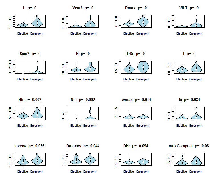
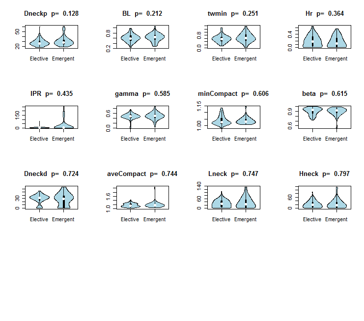
In order to describe the statistical variations of the covariates described in the Appendix, we plotted the vio- linplots [Hintze et al., 1998] for each one of them. Violinplot are boxplots that also contain an estimate of the density of the covariate in each of the groups. Figures 1 and 2 present the violinplots for the covariates. They are sorted by the p values obtained in a Mann-Whitney test, which are also presented.

Figure 1: Violin Plots for the variables derived from the computed tomography

4

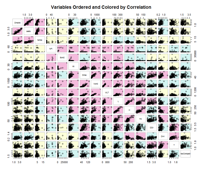
Figure 2: Violin Plots for the variables derived from the computed tomography In Figures 1 and 2, we see that many variables are important predictors of high risk of rupture when considered separately, especially measures related to the aneurysm’s size (such as length, volume and maximum diameter). In order to understand the relationship between them, Figure 3 shows the scatter plots of the 16 most significant variables on the Mann-Whitney test that was presented.

We see that many of the covariates are very correlated to each other. In what follows we try to consider them jointly by using different models for classification. The following models were implemented (for a reference

About These Models, See [Hastie Et Al., 2001]):

• (Sparse) L1 Regularized Logistic Regression (that is, choosing the coefficients that maximize P yi(β0 + βtxi) −log (1 + exp (β0 + βtxi)) −λ P |βi|). • (SparseL) Maximum Likelihood Logistic Regression with the variables with nonzero coefficients in the

Sparse Model

• (PC) Maximum Likelihood Logistic Regression with the first 5 Principal Components of the variables • (PCGAMs) Logistic Additive Model with the first 5 Principal Components of the variables, using smoothing

1−Μ(X) = Α + S(P1) + . . . + S(P5))

• (PCGAMl) Logistic Additive Model with the first 5 Principal Components of the variables, using local polynomials (1st order) (that is, the mean is modeled as log

1−Μ(X) = Α + L(P1) + . . . + L(P5))

• (AIC) Maximum Likelihood Logistic Regression with AIC criterion and stepwise selection

−2 D

N , where p is the number of covariates of the model and N

Is The Sample Size)

• (BIC) Maximum Likelihood Logistic Regression with BIC criterion and stepwise selection (BIC is P yi(β0+

Βtxi) −Log (1 + Exp (Β0 + Βtxi)) −(Log N)D)

• (AICPC) Maximum Likelihood Logistic Regression on the Principal Components with AIC criterion and

5

Figure 3: Scatter plots of the 16th univariately most significant variables • (RF) Random Forest (which is an average of de-correlated trees) Figure 4 shows the (cross-validated) estimates of the conditional misclassification probabilities as well as the estimate of the risk (expected cost) for the different models and different values of the cutoffs, as discussed in the previous section. Note that for the PCGAMl model, we have the bandwidth shown on the x axis rather than the cutofffor the logistic regression. For each value of bandwidth, we chose the optimal cutoff. Also, for the RF model, note that the same derivation from the previous section applies, once this is also a plugin estimator. For the sake of comparison, a vertical line is always displayed at the cutoff0.306, the optimal cutoffderived on the previous section. The cross-validated labels were obtained by using a random 12-fold cross-validation [Hastie et al., 2001].

Related Journal Articles & DOI Links

Selected peer-reviewed publications relevant to 12 Lead ECG Acquisition. Click the DOI to access the full paper (may require institutional access).

Why Choose Us?

Bangalore guidance for robotics, Spectre and autonomous systems projects.