Ansys Bone Screw Analysis

Paul-Ehrlich-Str. 31, Kaiserslautern, Germany

Abstract: Isogeometric Analysis (IGA) is a recently introduced computational ap- proach intended to breach the gap between the Finite Element Analysis and the Computer Aided Design worlds. In this work, we apply it to numerically simulate thermal expansion of oil free twin screw compressors in operation.

Figure: System Model & Simulation Flow for Ansys Bone Screw Analysis

High Global

smoothness of IGA leads to a more accurate representation of the compressor ge- ometry. We utilize standard tri-variate B-splines to parametrize the rotors, while the casing is modeled exactly by using NURBS. We employ the Galerkin version of IGA to solve the thermal expansion problem in the stationary case. The results allow to estimate the contraction of the clearance space between the casing and the rotors. The implementation is based on the open source C++ library G+Smo.

Figure: System Model & Simulation Flow for Ansys Bone Screw Analysis

This work is supported by the European Union within the Project MOTOR: Multi- ObjecTive design Optimization of fluid eneRgy machines. Keywords: Isogeometric analysis; Twin screw compressors; Thermo-mechanical coupling.

Figure: System Model & Simulation Flow for Ansys Bone Screw Analysis

Introduction

A twin screw compressor is a type of gas compressor with a great practical significance in various branches of engineering . In this work, we focus on the oil free subclass of these machines. The absence of oil and its cooling effect leads to a much higher temperature rise than in oil injected compressors. The resulting thermal stress distorts the shape of the rotors, making it necessary to increase clearances in order to avoid contact between the rotors. By considering the effects of thermal expansion in numerical simulations , an estimate of the minimal safe distance can be acquired and the efficiency of compressors could be increased.

Figure: System Model & Simulation Flow for Ansys Bone Screw Analysis

Here we propose an alternative approach to thermal expansion simulation with the use of Isogeometric Analysis (IGA), which is a modern computational method breaching the gap between the Finite Element Analysis and the Computer Aided Design worlds [3, 4].

Figure: System Model & Simulation Flow for Ansys Bone Screw Analysis

NURBS-based IGA is particularly attractive for applications with rotor-type geometries and where spinning motion is involved, due to its ability to exactly represent circular arcs. Another key feature of IGA is its high global geometric smoothness which allows to achieve greater accuracy per degree of freedom when modeling intricate shapes. In this paper, we demonstrate one possible strategy of generating 3D IGA models of the rotors and the casing. We start from the point cloud representation of the rotors’ profiles and approximate it with cubic B-spline curves. Using these approximations, the 3D tensor

Arxiv:1805.08848V1 [Math.Na] 22 May 2018

product B-spline parametrizations of the rotors are generated, while the casing model is built with NURBS. We then state a mathematical model of thermal expansion and use it to simulate thermal growth in the case of stationary rotors. The results are in a good agreement with the previous work, but much less computational resources are needed.

Figure: System Model & Simulation Flow for Ansys Bone Screw Analysis

We then use the results to estimate the contraction of the clearance space between the casing and the rotors. We give now a short overview of different simulation methods and aspects for twin screw compressors. One of the most common approaches, 0D chamber-model simulations, is described in the work by Kauder . For a systematic introduction to 3D CFD simulations we refer to Kovacevic et al. , while advanced CFD simulations including leakage flows are presented in [7, 8]. A novel efficient tool for fluid domain meshing is proposed by Hesse . In a recent work by Utri the optimization of screw machines with variable rotor pitch is addressed.

Figure: System Model & Simulation Flow for Ansys Bone Screw Analysis

This paper is organized as follows. In Section 2, we describe the creation of geometric models for the rotors and the casing. Section 3 deals with the mathematical model of thermal expansion and demonstrates its use on a numerical example. In Section 4, we draw conclusions and outline current and future research directions.

Geometric Models

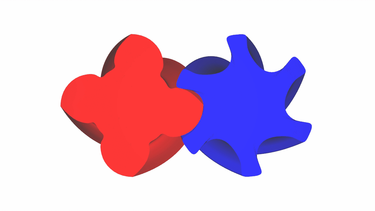
Both of the compressor rotors possess an intricate geometry (Fig. 1), a careful represen- tation of which is the focal point of this article. An extremely small clearance height between the rotors and the surrounding casing requires a high degree of accuracy from the approach chosen to describe these objects. The conventional approach is the use of point clouds. To run numerical simulations, however, another representation is necessary.

Within the framework of Isogeometric Analysis (IGA) the well-known tools from the world of Computer-Aided Design (CAD) - B-splines or NURBS - are utilized to model objects. However, unlike in CAD, not only the boundaries or surfaces of objects are modeled, but also their interior. The standard way to do this in IGA are tensor product B-splines.

Figure 1: Screw machine’s rotors. Throghout this article they are refered to as the male (left, red) and the female (right, blue).

Tensor Product B-Splines

To fix the notation, we shortly outline the construction of tensor product B-splines in the case of d = 2 dimensions. First we specify the polynomial degrees (p, q) and the horizontal

Ψ = {Η1 ≤Η2 ≤. . . ≤Ηn+Q+1} ,

which contain non-decreasing parametric real values so that

0 ≤Μ(Ψ, Η) ≤Q + 1

are the multiplicities of the parameter values in the knot vectors (the multiplicity µ(X, x) is zero if the given value x is not a knot in X). We write Mi,p(ξ) and Nj,q(η) for the univariate B-splines, which are computed by means of the recursion

(2)

for j = 1, . . . , n. Fractions with zero denominators are considered zero. The same recur- sion applies to Mi,p(ξ), replacing j, q in (1)–(2) by i, p for i = 1, . . . , m. A function f(ξ, η) : [ξp+1, ξm+1] × [ηq+1, ηn+1] →R2 is called a bivariate tensor product

(3)

with the de Boor control points di,j ∈R2, which form the control net associated to the parametric representation. In order to work with the unit square as parameter domain, combined with open knot vectors, we assume additionally ξ1 = . . . = ξp+1 = 0 and ξm+1 = . . . = ξm+p+1 = 1 at the beginning and at the end; analogously η1 = . . . = ηq+1 = 0 and ηn+1 = ηn+2 = . . . = ηn+q+1 = 1.

In d = 3 dimensions, a trivariate B-spline tensor product function is generated analogously,

(4)

with an additional set of univariate B-splines Lk,r and control points di,j,k ∈R3.

Model Construction

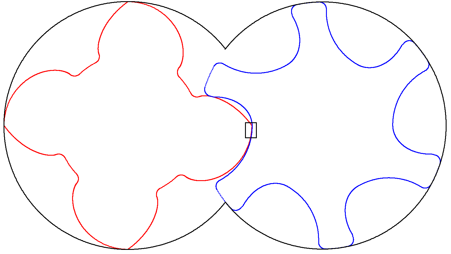
The geometry was originally provided in the form of a point cloud where the male and the female rotors of SRM type are described with 2572 and 2292 points correspondingly, see Fig. 2. It was scaled to match the configuration from . As a result, the axis distance is 80 mm, the clearance height is 44 µm between the casing and the rotors and approximately 100 µm between the rotors, the radius of the rotors is 50.97 mm. The difference in scales makes it challenging to come up with a B-spline approximation of rotors’ profiles without a large number of control points. That is one of the reasons why point clouds, rather than CAD models, are usually used to describe these objects.

We consider a B-spline approximation accurate enough if it deviates from the point cloud for less than 10% of the clearance height. This accuracy can be achieved by using cubic splines with 73 control points for the male rotor and with 109 control points for the female rotors. Four sharp corners of the male rotor are modeled by increasing the knots multiplicity. For the technical details of B-spline curve approximation we refer to .

Two circular arcs forming the casing can be modeled exactly by NURBS. This ability to exactly represent circular shapes makes IGA particularly suitable for applications where spinning motion is involved.

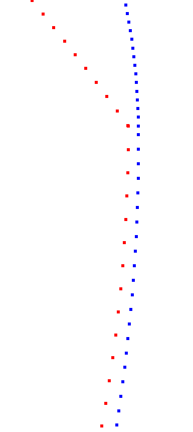
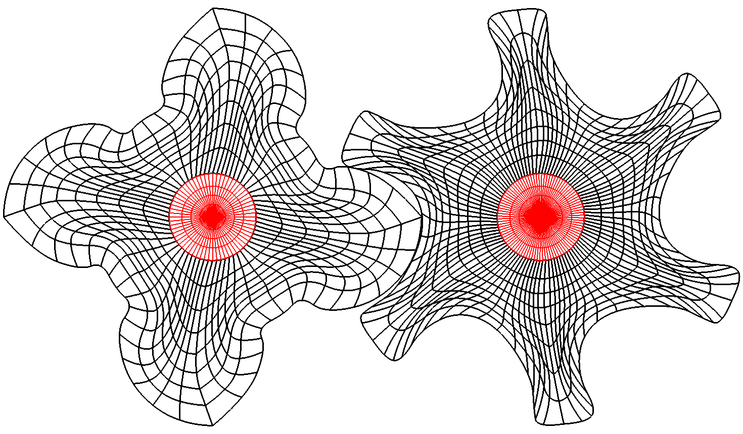
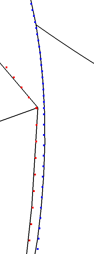
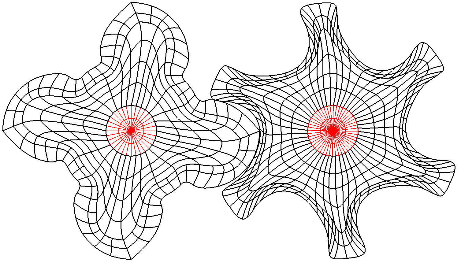
Figure 2: Point cloud describing the male and the female rotors as well as the surrounding casing. Magnified segment to the right clearly depicts the points and the clearance height. Next we generate 2D parametrizations for the cross-sections of the rotors. We choose the Scaled Boundary approach which is natural for rotary objects and allows to describe the interior of each rotor with a minimum number of patches, see Fig. 3. The outer layer is formed by ”scaling” the boundary towards the circular patch in the center. This central patch is later used to construct a shaft. The parametrization is C2-continuous inside the patches, but only C0 between them. Both patches are obtained as a geometric mapping from a unit square. For the central patch this mapping is not bijective at the center.

However, despite this singularity, this type of parametrizations is analysis-suitable. Optionally, the planar parametrizations can be locally refined or coarsened using THB- splines . By locally refining boundary layers of the rotors a finer resolution can be achieved there. This is especially attractive for the twin screw compressor example since the surfaces of the rotors require a finer resolution for analyzing and optimizing the mechanical properties. Figure 4 depicts a locally coarsened planar mesh. The B-spline approximation of the boundaries is maintained while less degrees of freedom are used in Figure 3: 2D scaled boundary parametrizations for the rotors. Original point cloud and its B-spline approximation (to the right, magnified).

the interior of the rotors. Figure 4: Local refinement with THB-splines allows to allocate degrees of freedom denser along the boundaries of the rotors than in their interior.

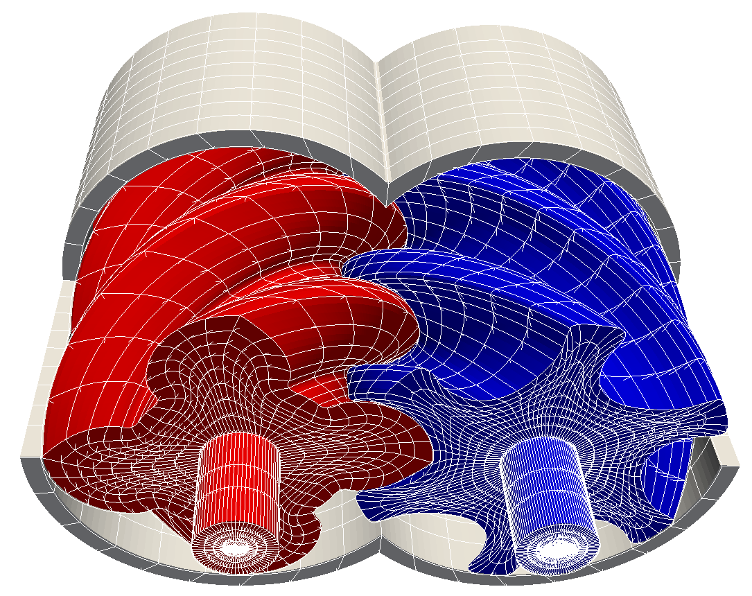
The final step is a 3D model. Each rotor is represented by a multi-patch geometry with 4 patches, see Fig. 5. The shaft has to be split into three parts so that the central part could have the matching boundary description with the inner surface of the outer layer.

The control points for the outer layer are obtained by combining several layers of rotated control points from the 2D cross-section. 20 layers of control points are used for both rotors. Both rotors have a length of 168.3 mm, the male is modeled with a pitch of 300◦, the female with -200◦. The shaft patches 2 and 4 are 30 mm long and the casing is 6 mm thick.

Figure 5:

3D models of the rotors and the casing.

Multi-Patch Structure Of The

parametrizations: each rotor consists of 4 patches with matching boundary descriptions.

Thermal Expansion

We consider here a very basic model of thermal expansion, which is nevertheless applicable for the case of screw compressors. It is based on the equations of linear elasticity, where the thermal growth is represented by an extra term. The use of a linear model is justified since only small deformations appear during the operation of the compressor, otherwise the machine would be blocked. However, these small deformations may still alter the shape of the clearing and change the efficiency of the compressor.

Mathematical Model

A body of isotropic material subject to a heat change from an initial temperature T0 to a temperature T expands or contracts uniformly in all directions . This can be modeled

(5)

where α is the coefficient of thermal expansion of the material and I is the d × d identity matrix. The resulting deformation is described by the displacement field u ∈Rd. To take into account the mechanical load as well we consider the linearized mechanical strain ε(u) := ∇(s)u, where ∇(s) is the symmetric gradient. We define the total strain εS(u) as

Εs(U) = Ε(U) + Εt = 1

2(∇u + ∇uT) + εT.

(6)

The total stress σ(εS(u)) is related to the total strain εS(u) by Hooke’s law with the Lam´e

Parameters Λ And Μ:

σ(εS(u)) = CεS(u) = 2µεS(u) + λtr(εS(u))I.

Related Journal Articles & DOI Links

Selected peer-reviewed publications relevant to 12 Lead ECG Acquisition. Click the DOI to access the full paper (may require institutional access).

Why Choose Us?

Bangalore guidance for robotics, Spectre and autonomous systems projects.