Ansys Drug Eluting Stent

arXiv:1805.06697v1 [cond-mat.stat-mech] 17 May 2018 Application of underdamped Langevin dynamics simulations for the study of diffusion

Shaked Regev1 And Oded Farago1, 2

2Ilse Katz Institute for Nanoscale Science and Technology, We use a one-dimensional two layer model with a semi-permeable membrane to study the diffusion of a therapeutic drug delivered from a drug-eluting stent (DES). The rate of drug transfer from the stent coating to the arterial wall is calculated by using underdamped Langevin dynamics simulations.

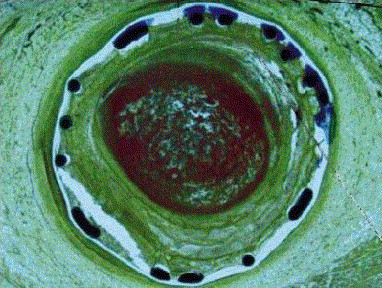
Our results reveal that the membrane has virtually no delay effect on the rate of delivery from the DES. The work demonstrates the great potential of underdamped Langevin dynamics simulations as an easy to implement, efficient, method for solving complicated diffusion problems in systems with a spatially-dependent diffusion coefficient.

Introduction

Arterial stents are indispensible in the treatment of coronary artery disease (CAD) and more specifically stenosis, the abnormal narrowing of blood vessels .

These stents are frequently implanted in arteries where blood flow has become precariously impeded. In recent decades, they have revolutionized the treatment of steno- sis by providing a safer alternative to coronary surgery.

In addition to diminishing the risk of major surgery com- plications, stents also facilitate recovery and avoid ad- ministering general anesthesia to patients . However, arterial stents have only been able to reduce the instances of recurring stenosis, or restenosis, to 20-30%, compared to 30-40% in coronary surgery .

In an effort to further curtail these rates, drug-eluting stents (DES) were introduced.

A Des Is A Stent

that uses programmed pharmacokinetics to release anti- proliferative pharmaceuticals into the arterial wall.

It

is comprised of a metallic strut coated with a poly- meric matrix or gel that encapsulates the therapeutic

Drug . The Drug Reduces Smooth Muscle Cell Growth

and prevents an inflammatory response - two predomi- nant causes of in-stent-restenosis and neo-intima prolif- eration . Stents coated in anti-proliferative agents have mitigated instances of restenosis to roughly 5% in clinical trials and are FDA approved .

Understanding the rate at which drugs are transported through the arterial tissue is crucial for stent design, and as such has been studied extensively . It has been identified that the major mechanism of drug transfer from the coating is diffusion through the arterial wall .

Thus, advective forces arising, e.g., from blood circula- tion in the arteries have been ignored in many models. The simplest model describing the system is based on the solution of a diffusion equation in a two-layer one- dimensional system. One-dimensional models represent a mathematical idealization of the three-dimensional stent geometry; nevertheless, they dominate the theoretical lit- erature on the subject because the drug release is pre- dominately along the normal direction to the stent axis whose dimension (the stent thickness) is much smaller then the lateral dimension (the stent radius). More com- plex one-dimensional models give weight to other phe- nomena and factors such as chemical reactions between the drug and the arterial wall , directed advection of the drug [7–9, 12–21], cell metabolism [16, 19], and the drug topcoat membrane permeability [6, 12, 14, 22, 23].

These phenomena and factors amend the partial differ- ential equations (PDEs) that describe the transport of the drug. They also modify the boundary conditions be- tween the layers and often require the introduction of additional layers [7, 8, 17, 20, 22, 24–27]. Some studies consider more complex two- [15, 26, 28] and even three- dimensional [13, 19, 22, 29, 30] geometries. The PDEs are often solved by separation of variables, or numerically through some kind of a discretization scheme, e.g., finite elements, finite differences, and the marker cell method.

Noteworthy exceptions include analytical Laplace trans-

Form Solutions , Boltzmann Reductions , And Nu-

merically solved Voltera integral equations . Experi-

Mental Data Is Also Available , And Has Been Used

to test and validate theoretical models. Layered systems, where in each region the diffusion co- efficient takes a different value, constitute a subclass of a more general class of systems with spatially varying diffu- sivity: D = D(x). Diffusion in such systems is described

(1)

where P(x, t) is the probability of being at coordinate x at time t, and J(x, t) = −D(x)∂xP(x, t) is the prob- ability flux. An alternative route for calculating P(x, t) is to numerically integrate the corresponding Langevin

(2)

where m and v denote, respectively, the mass and ve- locity of a diffusing particle.

Langevin’S Equation De-

scribes Newtonian dynamics under the action of two ef- fective forces: friction [first term on the r.h.s. of Eq. (2)]

2

and stochastic thermal noise (second term).

The Fric-

tion coefficient α(x) in (2) is related to the diffusivity D(x) in (1) via Einstein’s relation α(x) = kBT/D(x) [37, 38], where T is the temperature of the system and kB is Boltzmann’s constant. The stochastic noise, β, is chosen from a Gaussian distribution with zero mean ⟨β(x(t))⟩= 0, and delta-function auto-correlation ⟨β(t)β(t′)⟩= 2kBT α(x(t))δ(t−t′)[38, 39]. The probabil- ity density function (PDF) of the particle, P(x, t), can be computed from an ensemble of simulated trajectories, where the initial position of the particle at each trajec- tory is chosen from the intial PDF P(x, 0).

The Accuracy Of The Langevin Dynamics Simulation

method for computing P(x, t) depends largely on the quality of the discrete-time numerical integrator. Here (as in previous works ), we use the efficient and robust method of Grønbech-Jensen and Farago (G-JF) [35, 41] in combination with the “inertial” convention [38, 39] for choosing the value of α. In the absence of conservative forces from a potential energy gradient (which is the case discussed throughout this paper), the G-JF integrator

(4)

to advance the coordinate xn = x(tn) and velocity vn = v(tn) by one time step from time tn = ndt to tn+1 = tn + dt. In the above G-JF equations (3)-(4), βn+1 is a

And The Dampening Coefficients Of The Algorithm Are

b = [1 + (αdt/2m)]−1 ; a = [1 −(αdt/2m)] b.

(6)

Since the friction varies in space, the integrator must be complemented with a convention for choosing the value of α to be used in Eqs.(5) and (6) at each time step. The ambiguity concerning the appropriate choice of α is known in the literature as the “Itˆo-Stratonovich

Dilemma”. Here, We Use The Recently Proposed In-

ertial convention [38, 39] that assigns to α the value of the spatial average of α(x) along the inertial trajectory

(7)

where A(x) is the primitive function of α(x). We have previously demonstrated that while any reasonable con- vention for choosing α yields the correct PDF at the limit of infinitesimally small time step dt →0, the inertial convention gives very accurate results even for relatively large time steps. This property of the inertial convention stems from the fact that at small time scales, dt ≪m/α, the inertial trajectory serves as the leading approxima- tion to the actual path of the particle.

T=1000 (Eq. 8)

FIG. 1: The PDF of the two-layer problem (the vertical line at x = 0 represents the interface). Open circles and the solid line denote, respectively, the results of the Langevin dynam- ics simulations and the analytical solution Eq. (8) at t = 100.

Similarly, the open diamonds and the dashed line denote re- sults for t = 1000.

Assuming In Eq. (1) That 0 < D(X) < ∞(−∞<

x < ∞), the resulting P(x, t) (for t > 0) must be a continuous function for any initial condition. The flux j(x, t) = −D(x)∂xP(x, t) must also be continuous if no source or sink of probability are present in the system.

These properties of the PDF also apply to layered sys- tems where D is piece-wise constant. In this paper, we consider a simple one-dimensional two-layer model for a DES. Before arriving at that model, we first consider the simplest two-layer system, where D(x) = D1 for x < 0 and D(x) = D2 for x > 0. As just stated above, both the PDF and the flux must be continuous, including at x = 0, which sets the boundary conditions at the in- terface between the layers. Assuming that a particle is initially located at x = x0 > 0, i.e., P(x, 0) = δ(x −x0),

This Solution Can Be

interpreted as follows: For x > 0, the PDF is the outcome of two diffusion processes associated with (i) the original particle which has a unity weight and is located at x = x0, and an image particle of weight B located at x = −x0.

For X < 0, The Pdf Represents Diffusion Of An

image particle of weight A = 1 −B, which is located at x = x1.

Notice That For D1 = D2, We Have X1 =

x0, A = 1, B = 0, which reduces Eq. (8) to the well-

3

known Gaussian solution for a particle diffusing in an infinite space with constant diffusivity. Fig. 1 compares the PDF (8) for D1 = 1, D2 = 0.1, and x0 = 4 (lines) to the results of Langevin dynamics simulations based on the above described G-JF integrator with the inertial convention (symbols). In the simulations, we set m = 1 and kBT = 1. Thus, the friction coefficients in the layers are given by α1 = kBT/D1 = 1 and α2 = kBT/D2 = 10.

We set the time step to dt = 0.1. For both layers, this value of dt satisfies the condition dt ≤2m/α, which has been assumed in the application of the inertial convention for choosing ¯α (see discussion at the end of section I).

Fig. 1 depicts the PDF at t = 100 and t = 1000, based on 2.5 × 105 trajectories.

The Total Cpu Time Of The

simulations was 3 minutes on a PC. The agreement with Eq. (8) is excellent.

Interestingly, We Obtained Almost

identical results with dt = 4, which does not satisfy the condition for inertial dynamics. In the latter case, the total duration of the simulations was 5 seconds.

Two interesting limiting cases may be considered: For

(9)

which is the solution of the same problem with a reflect- ing wall at the origin. To simulate Langevin dynamics in the presence of a reflecting wall (located, without loss of generality, at x = 0), we follow the trajectory of the particle as computed by the Langevin integrator. If it crosses the wall, i.e., when xn+1 < 0, we simply relocate the particle at −xn+1 > 0, and reverse the velocity from vn+1 to −vn+1. The other limiting case is D2/D1 →0

(10)

which is the solution of the same problem with an ab- sorbing wall at the origin. When one simulates Langevin dynamics with absorbing boundaries, the trajectory is terminated when it crosses the boundary. Obviously, the total probability is not conserved but rather diminishes with time.

Semi-Permeable Membrane

Drug-eluting stents include a topcoat that influences the rate of drug release to the artery. Since the topcoat layer is thin compared to the dimensions of the stent and the arterial wall, it can be included in a DES two-

Layer Model As A Semi-Permeable Membrane Boundary

that controls the transition rate from the coating (first layer) to the artery (second layer). Let us first discuss the problem of diffusion across a semi-permeable mem- brane within the general context of two-layer systems.

We denote by Pcross the probability that, within a small time interval dt, a drug molecule arriving to the bound- ary from the first layer crosses it to the second layer.

Pcross =0.1

FIG. 2: The PDF at t = 100 of a particle starting next to a reflecting wall at the origin, and diffusing through a semi- permeable membrane at x = 10 (represented by the vertical line), with crossing probability Pcross. Squares, circles, dia- monds and stars denote the results of the Langevin dynam- ics simulations for Pcross = 1, 0.5, 0.25, 0.1, respectively. The solid line shows the solution for the case with no membrane [see Eq. (9)].

In the opposite direction (from the second layer back to the first), the crossing probability is unity. A semi- permeable membrane can be incorporated in Langevin dynamics simulations of layered systems in the follow- ing manner: Let us first consider the simpler case where the friction coefficient α is the same on both sides of the membrane, which is located at x = xm. We follow the particle until it crosses the membrane (xn < xm and xn+1 > xm).

In Order To Decide Whether The Particle

should cross the boundary or be reflected from it, we draw a random number, R, from a uniform distribution between zero and one.

If R > Pcross (Re-

flection). If α varies across the membrane, the algorithm is only slightly more complicated: The new coordinate and velocity (xn+1, vn+1) are computed assuming that the friction varies in space, i.e., with the inertial conven- tion for the average friction during the time step [Eq. (7)].

The step is accepted for R < Pcross and is changed to a reflection step for R > Pcross.

In The Latter Case, One

must take into account the fact that the particle has not passed the membrane and, therefore, the friction coeffi- cient along its trajectory remains constant. Therefore, the new coordinate and velocity are recalculated using the G-JF algorithm, with the already chosen value of βn+1, but with the friction coefficient at the initial co- ordinate xn < xm.

The Recalculated (Xn+1, Vn+1) Are

accepted if the particle has not crossed the membrane

If It

has. Fig. 2 shows simulation results for the PDF of a par- ticle, initially located right next at a reflecting wall at

Arterial Wall

Arterial Wall

FIG. 3: (A) A cross section of a stented artery, and (B) the corresponding one-dimensional two-layer model for drug re- lease from the stent to the artery.

x = 0, and diffusing in a medium with constant D = 1 that has a semi-permeable membrane at xm = 10. The PDF at t = 100 is plotted for various values of Pcross.

The PDF is discontinuous at xm because the membrane interferes with the diffusion rates. However, the mem- brane is not a probability sink or source and, therefore, the probability flux, j(x) = −D∂xP(x, t), arriving at the membrane from left (x →xm−) is the same as the flux leaving the membrane to the right (x →xm+).

This last feature of the PDF is visually apparent in Fig. 2. Since the membrane (partially) blocks the drug flow only from left to right, the probability density drops across the membrane, i.e., P(xm−, t) > P(xm+, t). The data in Fig. 2 suggests that the following relation holds: Pcross = P(xm+, t)/P(xm−, t). This relation is antici- pated from the continuity of the flux and the fact that for each Pcross molecules crossing the membrane from left to right, one molecule passes from right to left. For Pcross = 1, the membrane is effectively non-existent be- cause it does not impede the diffusion.

In This Limit,

P(x, t) becomes continuous at xm and is given by Eq. (9) with x0 = 0 (solid line in Fig 2).

The Model

Fig. 3 (A) shows a cross section of a stented artery with the struts in contact with the arterial wall. Fig. 3(B) illustrates the mapping of the system to the simple one- dimensional model discussed herein. The model consists of two layers representing, respectively, the coating and the arterial wall.

The First Layer (Coating), Which Has

length L1, is bounded between the stent strut (x = −L1) and the stent topcoat (x = 0). The former is a reflecting boundary, while the latter is a thin semi-permeable mem- brane. The second layer (the arterial wall) is of length L2. It is bounded between the topcoat and the adventi- tial side of the arterial wall (x = L2), which is modeled as an absorbing boundary since the drug arriving at the end of the artery is lost in the tissues adjacent to the adventitia. The first and second layers have diffusion co-

1/700

TABLE I: Model parameters and their physical (second col- umn), normalized (third column), and simulation (fourth col- umn) values.

efficients D1 and D2, respectively. We denote by m the mass of a drug molecule, and use the thermal energy kBT as the energy scale of the problem.

Typical values for the system parameters are given in the second column of Table I in MKS units. In the third column, the same parameters are given in normalized

Units, Where L1 = 1, D2 = 1, And Kbt = 1. Table I

also gives the physical and normalized values of the time

I /Di (I = 1, 2), Which Are The Characteristic

diffusion times in each layer. Notice the interesting fea- ture that these two time scales are of the same order of magnitude.

Using A Fictitious Mass

Another characteristic time scale appearing in table I is τm = mD/kBT , which is the crossover time from inertial to diffusive Langevin dynamics. This time scale, to be henceforth referred to as the ballistic time, is very impor- tant from a computational perspective since Langevin dy- namics simulations with the inertial interpretation must be run with time step dt < τm in order to appropriately simulate the transition statistics between the layers. In multi-layers systems, the limit on dt is set by the most viscous layer with the smallest diffusion coefficient and the smallest ballistic time. Therefore, in table I, we only give τm of the first layer. For the stent model, we have τm ∼10−18 sec, which is more than 24 orders of mag- nitude smaller than the diffusion times τ1 and τ2. This poses a huge computational challenge, as the aim of the study is to measure quantities like the rate of drug trans- fer to the bloodstream, which require simulations on time scales comparable to τ = τ1 + τ2. This implies that each simulated trajectory requires, at least, 1024 time-steps, which would make the simulations prohibitively time con- suming. More specifically, simulations of just 104 trajec-

1013 Years (!) Of Cpu Time On A

state of the art PC.

Related Journal Articles & DOI Links

Selected peer-reviewed publications relevant to 12 Lead ECG Acquisition. Click the DOI to access the full paper (may require institutional access).

Why Choose Us?

Bangalore guidance for robotics, Spectre and autonomous systems projects.