Ansys Fiber Orientation Heart

3D Scattered Light Imaging: Extracting 3D Fiber

orientations from 1D line profiles in brain imaging Dennis Scheidta, Charlotte Voßb, Cristian Rosero Ariasc, Santiago Saavedra Castanoc, Felix Matuschkea, Roxana Koojimansd,a, Katrin Amuntsa,e,

Arturo Susarrey-Arcec, Markus Axera,B

aInstitute for Neuroscience and Medicine 1, Forschungszentrum Juelich, Wilhelm-Johnen-Straße, Juelich, 52428, Germany

Wuppertal, Gaußstraße, Wuppertal, 42219, Germany

dNetherlands Institute for Neuroscience, Royal Netherlands Academy of Arts and Sciences, Meibergdreef 47, Amsterdam, 1105 BA, The Neatherlands

Abstract

Understanding the 3D fiber architecture of the brain at the microscopic scale is essential for revealing its structural connectivity and function. Polarization- based optical imaging (3D-PLI) techniques enable high-fidelity reconstruc- tion of single nerve fiber orientations but struggle to resolve fiber crossings, which are critical for recovering the full connectome. Scattering-based imag- ing provides access to the structure factor of three-dimensionally oriented fibers. By probing a fixed scattering angle under multiple azimuthal illumi- nation angles, in-plane fiber orientations and crossings can be recovered using computational scattered light imaging (SLI). However, despite containing 3D information, a theoretical framework to extract full 3D orientations has been lacking. In this talk, a simple analogical approximation of Rayleigh-Gans scattering theory is introduced to extract the 3D orientation of nerve fibers from one-dimensional SLI measurements. The theory is validated using tilted microscopic glass phantoms consisting of 2 µm-thick rod lattices fabricated by two-photon lithography. Finally, the method is applied to brain tissue samples and compared with 3D-PLI.

Keywords:

Scattered Light Imaging, Brain Imaging, 3D Imaging, Two

Arxiv:2609.03764V1 [Physics.Optics] 3 Sep 2026

Photon Lithography, Tissue Phantom, Polarized Light Imaging

1. Introduction

Mammalian brains consist of millions to billions of neurons that are intercon- nected through synapses and form highly complex structural and functional networks . Understanding brain function and behavior therefore requires a multiscale perspective, ranging from molecular and cellular organization to mesoscopic fiber architecture and macroscopic connectivity [3, 6].

While the cellular composition and many anatomical regions of the brain have been extensively characterized, the detailed reconstruction of neuronal connectivity remains challenging . In particular, mapping the trajectories and crossing patterns of nerve fibers at microscopic and mesoscopic length scales is still a major limitation. Diffusion tensor imaging (DTI) provides ac- cess to fiber orientations at the macroscopic scale, but its spatial resolution is insufficient to resolve microscopic fiber architecture . Optical meth- ods such as 3D-polarized light imaging (3D-PLI) and polarization-sensitive optical coherence tomography (PS-OCT) can reconstruct in-plane and three- dimensional nerve fiber orientations at microscopic resolution [4, 5]. These techniques exploit the birefringence of the myelin sheath surrounding nerve fibers. 3D-PLI has also been successfully applied to cortical tissue, where fiber densities and birefringence signals are considerably lower than in white matter .

However, birefringence-based methods have an intrinsic limitation in regions containing multiple crossing fiber populations. Since PLI measures the ac- cumulated retardation of the transmitted light field, the resulting signal rep- resents an effective orientation rather than the individual orientations of all contributing fiber populations. Consequently, two crossing fiber bundles with different in-plane orientations can yield a circular average of the underlying orientations, which prevents a direct separation of crossing fibers .

In contrast, Scattered Light Imaging (SLI) exploits the anisotropic scattering properties of nerve fibers. Nerve fibers can be approximated as cylindrical

September 4, 2026

structures that scatter light predominantly perpendicular to their symmetry axis. In SLI, the angular scattering response is measured by rotating an oblique illumination direction azimuthally around the sample . A single in-plane fiber orientation then gives rise to two characteristic scattering peaks in the angular profile . Since the measured intensity is approximately a linear superposition of the scattering contributions within one pixel, crossing fiber populations can generate multiple distinct scattering peaks. For exam- ple, two crossing in-plane fiber orientations can produce four peaks, allowing the individual orientations to be separated .

Previous simulations and experiments indicate that the angular scattering profile also contains information about the out-of-plane inclination of nerve fibers . However, a closed analytical description that directly relates the measured peak geometry to the three-dimensional fiber orientation has so far been missing. In particular, a model is required that links the angular peak positions and peak separations to the underlying in-plane orientation and inclination of cylindrical scatterers.

In this work, we introduce an analytical model based on the Rayleigh-Gans approximation for cylindrical scatterers to recover the missing inclination information from SLI measurements.

This Extends Sli From An In-Plane

orientation imaging technique toward a three-dimensional fiber orientation method, analogous in scope to 3D-PLI but with the additional ability to resolve crossing fiber configurations. The ground-truth orientation of brain fibers is generally not known a priori because of tissue complexity and inter- subject variability. Therefore, microscopic glass phantoms containing cross- ing cylindrical structures were fabricated using two-photon lithography to systematically investigate the relationship between fiber architecture and the measured SLI signal . The glass cylinders have diameters of 1 −2 µm to approximate the diameter range of large axons . These phantoms were measured under different tilting angles to emulate inclined nerve fibers and to validate the proposed analytical reconstruction method. Finally, the model is applied to a human brain section, and the reconstructed inclination is compared with inclination estimates obtained by 3D-PLI.

The results demonstrate that the Rayleigh-Gans model of a transparent cylin- der provides a suitable first-order approximation for describing the SLI signal in both glass phantoms and human brain tissue. Beyond the in-plane ori- entation of crossing fibers, the angular scattering profiles also contain infor- mation about the effective fiber diameter and inclination. In white matter, the reconstructed fiber diameters are substantially larger than in gray mat-

3

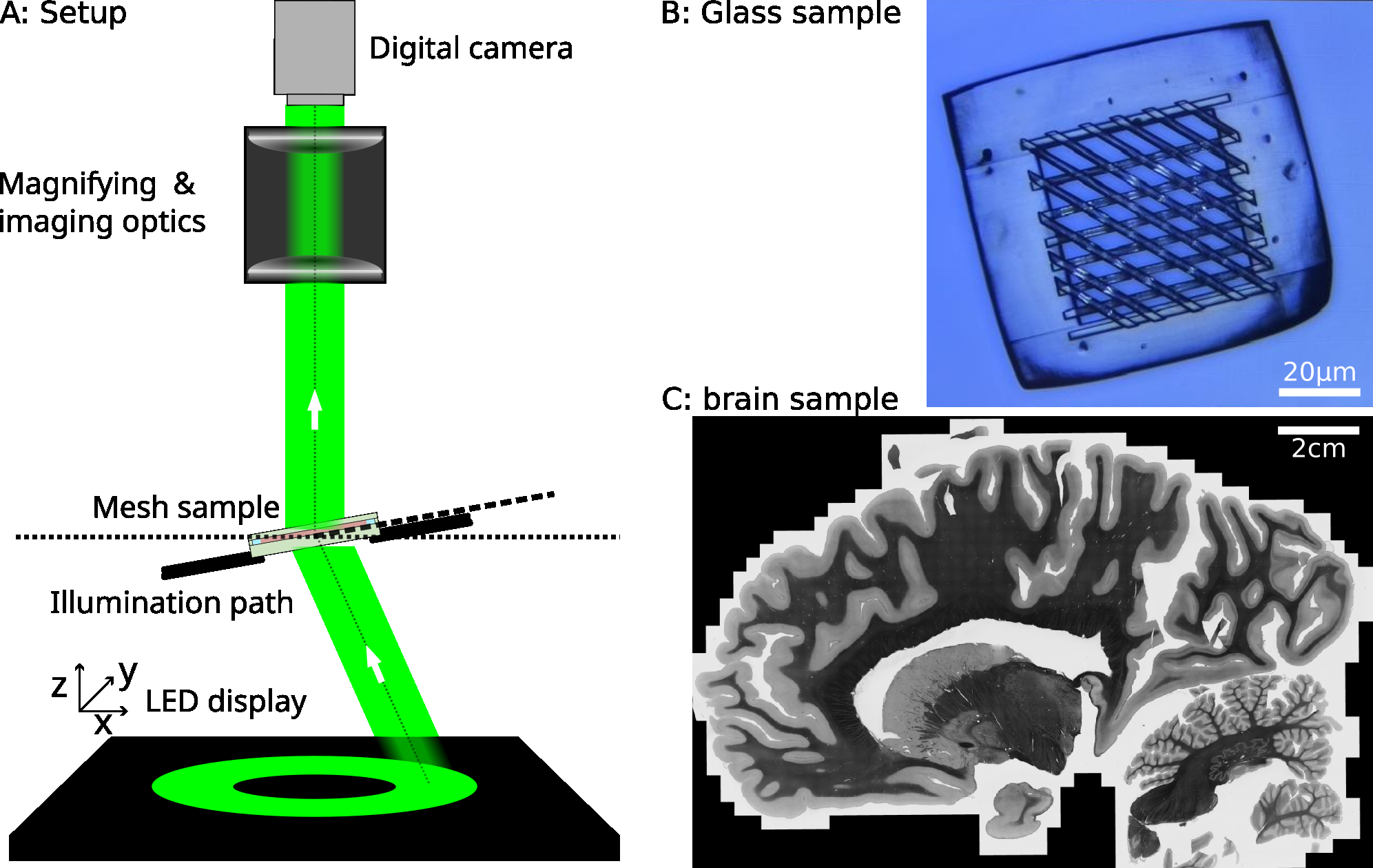
Figure 1: Experimental setup and used samples. A: Experimental setup with LED dis- play, sample stage, imaging lens and camera. The stage is rotated to simulate inclinated samples. B: Microscopic glass phantom created with two photon lithography. C: Sagittal human brain section.

ter, consistent with the expected anatomical composition. The inclination measurements show a strong correlation with 3D-PLI in white matter for low inclination angles. Remaining deviations may result from the different contrast mechanisms and angular sensitivities of the two imaging techniques and will be investigated in future work.

2.1. Setup

The measurements were performed with the setup illustrated in Fig.1. The optical system follows the general ComSLI configuration reported previously in [8, 16] and can also be operated for Mueller-polarimetric measurements.

In the present work, however, only the scattered-light imaging modality was used. Therefore, the polarimetric elements were positioned outside the rel- evant scattered-light detection path and are omitted from the schematic for clarity.

4

Oblique illumination was provided by a 46.56 × 46.56 cm2 LED display (IN- FILED s1.8 LE Indoor LED Cabinet, frame rate 2400 Hz).

The Display

contains 256 × 256 individually addressable RGB LEDs with a pitch of 1.8 mm and a viewing angle of 120◦. The sample was mounted 16 cm above the display, which corresponds to the focal distance of the imaging objec- tive. Annular illumination patterns were displayed with an inner radius of 50 LEDs and an outer radius of 90 LEDs, resulting in an approximate polar illumination angle of 45◦.

Image acquisition was performed with a Basler acA5472-17uc camera equipped with a Sony IMX183 CMOS sensor. The sensor has 5472 × 3648 pixels with a pixel size of 2.4 × 2.4 µm2. A QIOPTIQ APO-RODAGON-D 1X 75/4.0 objective was used for imaging, yielding a field of view of approximately 8×5 mm2 and an effective object-space pixel size of about 1.5 µm. The optical resolution was estimated to be 2.19 µm using a USAF resolution target. To maximize the collected scattered-light signal, the camera aperture was fully opened to a diameter of 5.6 mm.

For all measurements, only the green LEDs of the display were used, en- abling comparability with previous ComSLI experiments performed under green illumination . The exposure time was set to 0.5 s for the Hadamard sampling scheme described in . Camera gain was not applied, and the analysis was restricted to the green channel of the recorded images.

For tilted measurements, the sample stage was placed on a optical post mount and fixated at the vertical axis. Then the stage was rotated in steps of ∆ϵ = 5◦from ϵ = [0◦, 70◦]. Tilt positions were verified with a digital lever (Stabila TECH 196 DL). After ϵ = 70◦no further measurements were possible, as the stage then blocks the illumination part partially, so that the sample is not illuminated from all sides anymore. A brain tissue sample was measured in a Polarization Microscope LMP3D (Taorad GmbH, Aachen, Germany) .

There, first the PLI measurement with 5 different tilts of the illumination path were conducted.

Afterwards, A Customized Led Ring With N = 32

LEDs performed the SLI measurement. The whole section was scanned and stitched using an in-house stitching algorithm.

2.2. Sample Preparation

Two samples were investigated. First, a glass phantom fabricated by two- photon lithography was used to validate the scattered-light signal model: A custom made silicon loaded photoresin formulation was prepared under

5

yellow light conditions to reduce UV exposure and prevent undesired poly- merization. POSS and PETA were mixed in a rotary evaporator operated under reduced pressure at 75 °C, and 140 rpm. After having those compo- nents homogeneously mixed, DETC was dissolved in DMAc with a vortex mixer and then transferred to the POSS and PETA mixture. The mixing continued for another hour, but under ambient pressure. The final yellow- colored photoresin was pipetted into 25 mL amber bottles (Duran) and used directly to obtain the pre-glass mesh microarchitecture employing a Two Photon Litography (TPL) direct laser writing system (Photonic Professional GT, Nanoscribe) operated in the DiLL mode. A 25×/0.8 objective (Imm Corr DIC M27, LCI Plan-Neofluar; Carl Zeiss) focused the femtosecond laser radiation focal spot on the resin using differential interference contrast. For this printing, an ITO-coated glass slide (2.4 cm × 3.2 cm) was used as a substrate to keep the microarchitectures in place. Finally, the TPL printed microstructure, together with the substrates, were placed in open-cap ce- ramic crucibles and then transferred into an air chamber oven (LH 15/12, Nabertherm). The thermal processing was conducted at 650 °C to combust the organic constituents from the composite polymer and transform the 3D mesh into the desired glass. More details on the fabrication process can be found in . The microstructure consists of nearly cylindrical glass rods with a diameter of 2µm, arranged at a predefined crossing angle of 45◦(see Fig.

1 B). To reduce diffraction artifacts caused by periodic grating-like arrange- ments, the rod positions were randomized using Poisson-disk sampling with a minimal distance of 5µm. The rods were embedded in a rectangular glass frame with a thickness of 20µm, which provided mechanical stability during the cooling-induced shrinkage process after fabrication.

Second, a sagittal section of a human brain was investigated.

The Post-

mortem brain sample (female, 80 years old) was formalin-fixed and deep- frozen as described above. The frozen brain was cut into 60 µm-thin sections which were mounted in a 20% glycerol-water solution in between coverslips.

One section was selected for this study (see Fig. 1 C). Detailed preparation protocols are described in . This study was conducted in accordance with all applicable ethical regula- tions. The body donor provided written informed consent for the general use of post-mortem tissue for research and educational purposes. The use of the brain was approved by the Netherlands Brain Bank (ethics approval NBB-1037/2018), in the Netherlands Institute of Neuroscience, Amsterdam, the Netherlands.

2.3. Signal Model Of A Cylindrical Scatterer

The diameter of myelinated axons is distributed approximately in the range of d = [0.5−10]µm, with an average value of davg ≈1µm . This is on the order of the illumination wavelength λ = 530nm. Consequently, the scat- tering process cannot, in general, be described by simple geometric optics.

Instead, the interaction of light with axons has to account for wave-optical effects such as interference, multiple internal reflections, and scattering from finite-sized dielectric structures . A full description would require Mie-type scattering theory. However, for finite cylindrical structures and the specific illumination–detection geometry used here, closed analytical solutions are not available in a form suitable for large-scale image analysis. Numerical so- lutions of the corresponding scattering problem are computationally expen- sive and therefore inefficient for pixelwise reconstruction in large microscopy datasets.

A tractable approximation is provided by the Rayleigh-Gans (RGS) theory, in which the scattering object is approximated as a continuous distribution of weakly scattering dipoles. This approximation is valid under the condi- tion kd|∆n| ≪1, where k = 2π/λ is the wave number and ∆n = nm −ns is the refractive-index difference between the surrounding medium nm and the sample ns. In brain tissue, typical refractive indices are in the range ns ≈1.36 −1.42, while the mounting medium used here, a 20% glycerol- water solution, has approximately nm = 1.36. Thus, |∆n| ≈0.01−0.06 ≪1.

Although the Rayleigh-Gans condition is most strictly fulfilled for smaller axon diameters and weak refractive-index contrasts, the approximation pro- vides an analytically accessible model that captures the dominant angular structure of the scattering pattern.

For unpolarized light, which is used in the experiments, the scattered inten- sity Iscat of a cylindrical scatterer can be expressed as

(1)

where θscat is the scattering angle, r is the cylinder radius, h is the cylinder height, R is the distance between the scatterer and the detector, I0 is the incident intensity, and D(θscat, γ) is the form factor of the scatterer. The form factor is obtained by integrating over the circular cross-section of the

Which Yields

D(θscat, γ) = sinc (kh sin(θscat/2) cos γ) J1(2kr sin(θscat/2) sin γ)

Kr Sin(Θscat/2) Sin Γ

.

(2)

In this expression, the sinc term describes the axial contribution of the cylin- drical scatterer, while the Bessel term J1(r)/r describes the radial contribu- tion. The remaining geometrical quantities, namely the scattering angle θscat and the effective angle γ, can be derived by describing both the incident light direction and the cylinder orientation in spherical coordinates. Here, α and β denote the azimuthal and polar angle of the incident light, while ϕcyl and θcyl denote the azimuthal and polar orientation of the cylinder.

For the specific imaging geometry of the setup shown in Fig. 1A, the scat- tering angle is given by Θscat = β. The effective angle γ between the cylinder

Axis And The Scattering Vector Is Then Given By

γ = arccos (−cos θcyl sin(β/2) + sin(θcyl) cos(β/2) cos(α + ϕcyl)) .

(3)

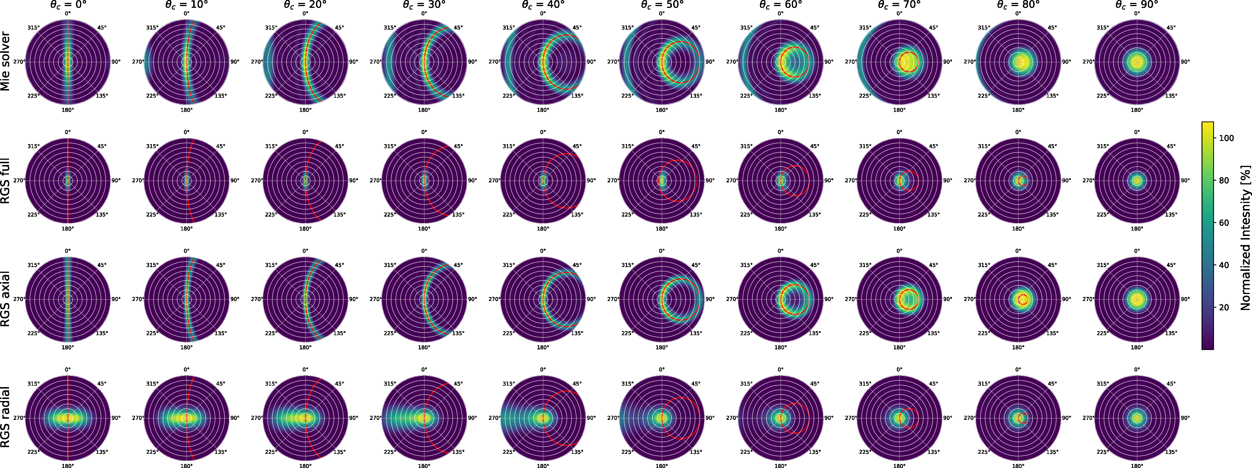
Figure 2 compares the scattered intensity of a cylinder with r = 500nm and h = 1µm for a numerical Mie-type solution obtained with the ADDA solver and for the RGS model described by Eqs. 1, 2, and 3. Different inclination angles θcyl are shown for a fixed in-plane orientation of ϕcyl = 45◦.

In the polar plots, the radial axis corresponds to the scattering angle Θscat = β, while the polar axis corresponds to the illumination azimuth α. The RGS solution is separated into its radial and axial contributions. The red lines indicate the expected positions of the scattering maxima according to conical diffraction theory . Experimentally measured angular scattering profiles correspond to samples taken at a fixed polar angle.

The comparison shows that the radial contribution of the RGS model mainly damps the signal with increasing polar angle and remains approximately con- stant for a fixed polar angle. Therefore, for the angular profiles measured at a fixed scattering angle, the dominant angular modulation can be described by the axial sinc2 term. This becomes particularly clear when comparing the RGS model with the numerical Mie-type solution. The main angular structure of the scattering pattern is reproduced by the axial sinc2 contribu- tion, and the positions of the maxima agree well with the maxima predicted by conical diffraction theory. This indicates that the simplified analytical model is suitable for describing the peak positions in the measured angular scattering profiles.

8

Figure 2: Scattering patterns of a single cylinder with radius r = 500, nm and height H = 1µm for the illumination geometry shown in Fig. 1A. The cylinder inclination θcyl increases from 0◦on the left to 90◦on the right in steps of 10◦. The first row shows the numerical solution obtained with the ADDA solver . The second row shows the corresponding result calculated from the full Rayleigh–Gans scattering (RGS) expression in Eq. 2. The third and fourth rows show the isolated contributions of the axial sinc2 term

And The Radial Bsinc2

1 term, respectively. The angular coordinate denotes the azimuthal illumination angle α, whereas the radial coordinate denotes the polar illumination angle β. In the experiments, angular scattering profiles are sampled at a fixed polar angle β while varying the azimuthal angle α.

With increasing inclination θcyl, the scattering pattern changes from a nearly straight line to a curved structure. The ends of the curve shift toward the inclined side of the cylinder, in agreement with the observations reported by Menzel et al. . Consequently, if the scattering angle Θscat, or equivalently β, is known, the inclination can be reconstructed from the angular peak sep- aration ∆αs in the measured SLI profile. Solving the peak-position condition

#

.

(4)

In the original RGS expression, the physical cylinder height h appears in the argument of the axial sinc2 term. For nerve fibers, however, the physical length can range from several micrometers to centimeters and is therefore much larger than both the fiber diameter and the optical resolution. Two interpretations are possible. First, the effective height could be limited by the camera pixel size and the optical magnification, such that the finite detection area defines the relevant scattering length. Second, for elongated fibers with

9

h/r ≫1, the fiber can be treated as effectively infinite along its axis. In this case, the finite transverse extent of the fiber becomes the dominant geometrical scale that determines the observed angular peak width. Under this effective-cylinder interpretation, the diameter of the cylinder or nerve fiber enters the sinc2 term as the relevant structure size.

Under this assumption, the cylinder diameter can be estimated from the measured peak width. Solving the sinc2 profile for the Full Width at Half

2 K Wfwhm

.

(5)

Here, wFWHM denotes the angular full width at half maximum of the scatter- ing peak. Applying this relation to previous Hadamard-based experiments indicates that the observed peak width cannot be explained by the ef- fective camera pixel size alone. In these experiments, strong peaks with a FWHM of approximately 3 · 360/64◦were observed, corresponding to an es- timated diameter of D ≈5µm. This value is larger than the effective pixel resolution of ∆x = 1.5µm and therefore supports the interpretation that the peak width contains information about the physical transverse structure size rather than being solely limited by the imaging pixel size.

2.4. Peak-Pair Attribution Algorithm

A single fiber population can generate up to two scattering peaks in the angular SLI profile. The angular separation of these peaks, ∆αs ∈[0, 180]◦, depends on the fiber inclination according to Eq. 4. For a single predominant fiber orientation within a local tissue region, the inverse problem is therefore comparatively well constrained: the in-plane orientation is determined by the angular position of the peak pair, while the inclination is inferred from the peak separation. However, when multiple fiber orientations are present within the same region, the individual scattering contributions are approxi- mately linearly superposed. For M different fiber orientations, up to j = 2M peaks may therefore be expected. Since peaks from different fiber popula- tions can overlap, merge, or fall below the noise floor, the actually observed number of peaks can vary between j = 1 and j = 2M.

In practice, the attribution problem is limited to at most M = 3 fiber ori- entations, corresponding to up to six detectable peaks. This restriction is motivated by both the finite angular sampling of the SLI profile and the expected biological complexity of the investigated tissue. For a profile with

10

N = 32 angular measurements, resolving and assigning more than six peaks would lead to a strongly underdetermined combinatorial problem. Moreover, crossing regions in white matter typically contain two dominant fiber orien- tations and only rarely require three [15, 12]. In cortical myeloarchitecture, the dominant anisotropic scattering signal is also often described by a mesh- like arrangement of a small number of local orientations . More complex configurations may occur in gray matter, but the reduced axon density in this region results in a weak anisotropic signal, such that reliable attribution of many individual peak pairs becomes increasingly noise-limited.

The measured angular profile I(α) is modeled as a linear superposition of

(6)

where B(α) denotes a slowly varying background, Am is the amplitude of the m-th contribution, and Tm is a symmetric peak-pair template with orienta- tion ϕcyl,m, peak separation ∆αs,m, and angular width wm. The two peak

2

mod; 180◦.

(7)

Equivalently, for two detected peak positions αi and αj, the axial peak sep-

(8)

and the corresponding candidate orientation ϕcyl,m is estimated from the axial midpoint of the two peak positions. The inclination is then obtained

By Inserting ∆Αij

s,m into the inverse relation of Eq. 4. The attribution procedure first detects local maxima in the angular profile and characterizes each peak by its position, prominence, and width. All geo- metrically admissible peak pairs are then generated from the detected peaks.

Candidate pairs are rejected if their separation is outside the physically mean- ingful range or if they violate minimum angular-distance constraints. Each remaining pair receives a score based on peak prominence, approximate sym- metry, peak width, template agreement, and consistency with the expected

11

number of fiber populations. The best set of non-conflicting peak pairs is then selected by minimizing a combined attribution cost:

(9)

where NRMSEm measures the residual between the local profile and the peak-pair template, Pm represents the combined peak prominence, Sm penal- izes asymmetric or implausible peak-pair geometry, and Om penalizes invalid overlap or duplicate assignments. The constants λr, λp, λs, and λo weight the individual criteria.

Special care is required for overlapping peaks. If one observed maximum is shared by two candidate peak pairs, the shared peak is only accepted if it is sufficiently broad. This constraint is motivated by simulations showing that true peak superposition produces a widened peak, whereas isolated sharp maxima are more likely to represent individual peaks or noise-induced de- tections. Therefore, sharp but prominent peaks are allowed to form ordinary peak pairs, but they are not used as shared peaks between multiple orienta- tions. Only peaks whose angular width exceeds a predefined threshold are considered valid shared-peak candidates. This prevents the attribution al- gorithm from explaining several fiber orientations by repeatedly reusing the same narrow peak.

The output of the peak-pair attribution step consists of initial estimates for the in-plane orientation, inclination, and diameter of each selected fiber population.

3.1. Signal Characterization At Glass Phantoms

To characterize the scattering signal at intersecting structures, the crossing angles of the glass phantoms are determined using SLI and compared with the theoretically expected values. The glass phantoms used have predefined crossing angles of 90°, 60°, 45° and 30°, which also allows the influence of the crossing angle on the SLI signal to be investigated. As both glass rods and axons are described as transparent cylinders in the model used, the findings can, in principle, be extrapolated to brain tissue.

The glass phantoms are measured within the SLI setup and masked according to their averaged intensity, resulting in an individual mask for each phantom.

Related Journal Articles & DOI Links

Selected peer-reviewed publications relevant to 12 Lead ECG Acquisition. Click the DOI to access the full paper (may require institutional access).

Why Choose Us?

Bangalore guidance for robotics, Spectre and autonomous systems projects.