Ansys Gradient Induced Heating

3D-1D modelling of cranial mesh heating induced by low or

Abstract

Background and Objective: Safety assessment of patients with one-dimensionally structured passive implants, like cranial meshes or stents, exposed to low or medium frequency magnetic fields, like those generated in magnetic resonance imaging or magnetic hyperthermia, can be challenging, because of the different length scales of the implant and the human body. Most of the methods used to estimate the heating induced near such implants neglect the presence of the metallic materials within the body, modeling the metal as thermal seeds. To overcome this limitation, a novel numerical approach that solves three-dimensional and one-dimensional coupled problems is proposed.

Methods: The proposed method is compared with measurements performed on a cranial mesh exposed to the magnetic field generated by a gradient coil system for magnetic resonance imaging. Then, it is applied to a magnetic hyperthermia case study in which a patient with a cranial mesh is exposed to the magnetic field generated by a collar-type magnetic hyperthermia applicator for neck tumour treatment.

Results: The experimental comparison of the proposed method predictions and the measure- ment data shows an improved accuracy near the maximum temperature increase up to 25 % with respect to the method based on thermal seeds. The application of the proposed method applied to the magnetic hyperthermia case study leads to a prediction of the maximum temperature increase that is 10 % lower than the one overestimated by relying on thermal seeds. At the same time, the proposed method corrects the underestimation of the thermal seeds in the regions where the electromagnetic power is not directly deposited and the temperature increase is only due to heat transfer.

Conclusions: The proposed method leads to improved results with respect to previous ap- proximations by modelling the thermal diffusion through the highly conductive metallic implants without affecting the anatomical human model discretization based on voxels.

Keywords: Bioheat equation, Finite element method, 3D-1D coupling, Magnetic hyper- thermia, Magnetic resonance imaging, Medical implant

Introduction

Medical technologies based on magnetic fields are, nowadays, common tools both in diagnostic and in therapeutic clinical practice. A noteworthy example from diagnostics is magnetic resonance imaging (MRI) , which exposes the patient simultaneously to three different magnetic fields : a stationary ‡Istituto Nazionale di Alta Matematica F. Severi, 00185 Roma, Italy

Arxiv:2504.16600V2 [Cs.Ce] 13 Aug 2025

field, typically equal to 1.5 T or 3 T; a radiofrequency (RF) field, whose frequency, typically of 64 MHz or 128 MHz, depends on the stationary field intensity; and a gradient field, whose time-dependent waveform has a frequency bandwidth ranging from about 100 Hz up to a few kilohertz.

From the therapeutic side, a promising emerging technology is magnetic hyperthermia (MH) for cancer treatment . It is based on the experimentally observed positive effect of heat against cancer . In MH, tissue heating is obtained through magnetic losses induced by an alternating magnetic field in magnetic nanoparticles (MNPs), which acts as thermal seeds, injected in the tu- moural region. The magnetic field applicators used in this context commonly operate in the low RF range, from 100 kHz to 300 kHz .

A critical step in the procedure that leads to the clinical adoption of medical technologies based on the exposure of patients to magnetic fields is their safety assessment. For patients, the strict limitations introduced for workers and general public exposure in the ICNIRP guidelines [5, 6] should not hold by default, because the benefit-risk principle in a clinical setting is different than in other scenarios. Nonetheless, regulatory agencies discipline the exposure of patients to fields generated by medical devices. MRI equipment, for instance, is regulated by the IEC 60601-2-33 standard , which provides indications for all three fields to which the patients are exposed, to limit the possible occurrence of magnetophosphenes, temperature increase, nerve stimulation, and so on. Regarding MH, instead, the definition of regulations is still ongoing and will deal with the injectable MNPs as well as the magnetic field applicator . For the latter, the Atkinson–Brezovich limit, forcing the product between the maximum intensity of the generated magnetic field H and its frequency f to comply with the constraint Hf < 5 × 109 A m−1 s−1 , is currently adopted as a rule of thumb to guarantee no thermal stress in the tissues where the MNPs are not present. Nonetheless, evidences collected from the literature show that in certain cases this limit could be largely exceeded without inducing thermal damages outside the target region .

Since the fourth edition of IEC 60601-2-33 has been published in 2022 , some indications about patients with implantable medical devices have been included. This addition became necessary because of the increasing number of medical implants within the population. The presence of metallic, electrically conductive components in the patient’s body could lead to complicated interactions with the magnetic field that should be taken into account to guarantee a safe MRI examination .

The complicated interaction could take place also with the magnetic field generated by the MH applicator, in which case the Atkinson–Brezovich limit does not provide a reliable safety condition. To avoid unquantified risks, the presence of implants is currently used as an exclusion criterion for MH treatment, affecting a large portion of candidates . In particular, in MH the risk originates from the Joule losses due to eddy currents induced by the magnetic field in the implant metallic components. The heat deposited in that way diffuses by thermal conduction from the implant to the surrounding biological tissues, causing an undesired temperature increase . The same physical effect is found in the interaction between a metallic implant and the gradient field of MRI [11, 13], although currently it is regulated only for active implantable medical devices (AIMDs) by ISO/TS 10974 . The feasibility of extending the prescriptions of this technical specification to passive implants is under investigation [15, 16, 17].

To assess safety conditions in presence of metallic implants, mathematical and numerical mod- elling are invaluable tools, which open the way to in silico trials . In the context of electromag- netic dosimetry, in silico trials are particularly important, because they can predict power losses and thermal stresses generated within the human body, avoiding invasive and potentially dangerous mea- surements. More specifically for medical devices, in silico trials were recently strongly legitimated by the first computational Medical Device Development Tool qualified by the US Food and Drug Administration (FDA) , to support MRI RF safety testing of AIMDs.

Despite the large availability of powerful computational tools, also in commercial software, it remains a challenge to obtain reliable results in certain specific scenarios. In particular, the topic of this paper is looking for a proper in silico assessment of thin (one-dimensionally structured) implants, which pose a challenge for their numerical modelling because of the different length scale of their small diameter (usually lower than 1 mm) compared to the human body size. It has been shown in the literature that good numerical solutions can be obtained by relying on non structured tetrahedral

2

discretizations . However, heterogeneous anatomical human models are usually provided in voxel- based discretizations , which can be directly obtained from MRI segmentations . A proper discretization of a thin metallic implant with voxels forces the adoption of extremely fine grids, leading to large computational costs and hardware resources .

This paper will focus on the modelling of passive implants with a one-dimensional structure, like metallic stents or metallic cranial meshes . In this case, the presence of closed loops makes the implant subject to the induction of eddy currents when exposed to time-varying magnetic fields, like those generated by the MRI gradient coils (GCs) or the MH applicator. Because of the large conductivity value of metal with respect to biological tissues, a proper estimation of the eddy currents induced by low or medium frequency magnetic fields can be obtained by taking into account only the implant and neglecting the surrounding tissues. This observation led to the recent proposal of a purely one-dimensional model based on a circuital description of the implant . Although this approach provides an accurate estimation of the Joule losses within the implant, a further step is needed to assess the thermal effects in the surrounding biological tissues. To avoid the adoption of an extremely fine voxel-based discretization of the computational domain, recent publications dealing with this topic neglect the thin metallic implant in the thermal assessment [23, 24].

Precisely,

they model the implant as a set of thermal seeds, so that the previously computed Joule losses are distributed directly within the voxels of biological tissues. The temperature increase is finally computed according to Pennes’ bioheat equation .

Since the heating due to the Joule losses is not, in general, uniformly distributed within the metallic implant, the modelling approach based on thermal seeds is lacking of a physical contri- bution: thermal conduction through the implant itself.

Being Metals Good Thermal Conductors,

this contribution could significantly affect the final temperature distribution. To take this contri- bution into account, relying on a voxel-based discretization of the biological tissues and keeping the computational burden reasonably low, numerical approaches addressing the coupling between three-dimensional and one-dimensional (3D-1D) problems on non-conforming discretizations can be adopted. We here decide to adopt the optimisation-based domain decomposition approach recently presented in [26, 27]. Under this approach, auxiliary variables are introduced at the interface and a cost functional, mimicking the error committed in the fulfillment of interface conditions, is minimized constrained by the set of 3D-1D partial differential equations (PDEs). A similar optimisation-based 3D-1D coupling strategy was already applied successfully to the simulation of fluid and chemical ex- changes in tumor-induced angiogenesis . Different strategies to address 3D-1D coupled problems can be found in the literature, such as in , relying on weighted Sobolev spaces, , based on proper averaging operators, , resorting to kernel functions to approximate the singular behavior in a neighbourhood of the 1D inclusions, and , in which the 3D and the 1D problem are coupled by means of Lagrange multipliers.

In this paper, the optimisation-based 3D-1D coupling strategy is used to assess the heating induced by exposing the metallic grid of a cranial mesh to a low or medium frequency magnetic field. A comparison of the numerical results with experimental temperature measurements performed by exposing the cranial mesh to a system of MRI GCs is presented. Finally, the proposed method is applied to a MH case study problem, in which a patient implanted with a cranial mesh undergoes a MH treatment for a neck superficial tumour.

Mathematical And Numerical Modelling

The problem to be modelled is the heating of a filamentary medical implant with closed loops induced by a low or medium frequency magnetic field. Hence, the computational domain is a portion of the human body, Ω⊂R3, with an implanted medical device, Σ ⊂Ω. We assume that the filamentary implant Σ is a network of thin tubular metallic wires with constant radius r. Moreover, the implant is assumed to have a one-dimensional structure, in the sense that the radius r is much smaller than the characteristic lengths of the implant itself and of the domain Ω. As a consequence, each wire of

3

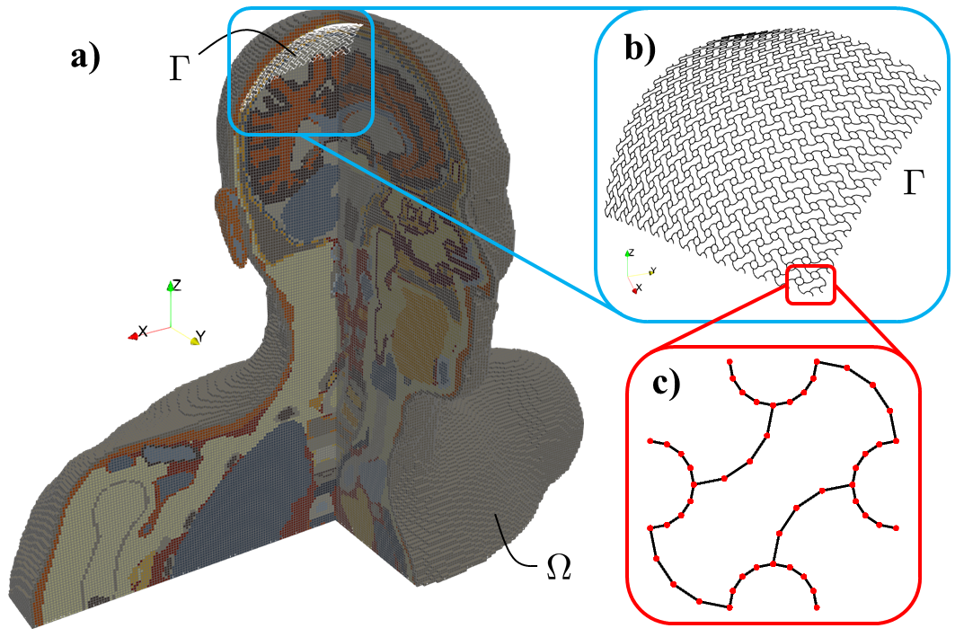
Figure 1: Sketch of a computational domain. a) The voxel-based anatomical human model Glenn, from the Virtual Population , is the computational domain Ω. b) The one-dimensional network Γ models the cranial mesh implanted in Glenn. c) The detail of the cranial mesh highlights the piecewise linear approximation in its geometry description (the red dots connect adjacent seg- ments).

Σ can be approximated by its axis to get the one-dimensional network Γ ⊂Σ, which will be used as the 1D representation of the filamentary implant in the following 3D-1D coupled model. A sketch of the computational domain Ωand of the implant model Γ is provided in Fig. 1 with reference to the case of a cranial mesh.

The problem involves two physical models solved in cascade. First, the electrical currents induced within the implant are evaluated through an electromagnetic model, previously presented in and summarised in Section 2.1.1. The resulting Joule losses are, then, used as forcing term of the thermal model, described in Section 2.1.2.

Electromagnetic Model

It is assumed that the frequency of the magnetic field is sufficiently low so that: the secondary magnetic field due to the currents induced within the biological tissues is negligible with respect to the primary field; the induced displacement currents are negligible with respect to the induced conduction currents.

These are reasonable approximations for frequencies up to about 1 MHz .

Under

this assumption, the large difference between the conductivity of metallic implants (of the order of 1 MS m−1) and the one of biological tissues (of the order of 0.1 S m−1 ) leads to eddy currents that are confined within the implant. Therefore, the computational domain of the electromagnetic problem can be limited to just the one-dimensional model Γ of the filamentary implant.

From the computational viewpoint, the assumed approximations allow one to handle Γ as an electrical network, whose nodes (the red dots in Fig. 1c) are connected by branches (the black segments in Fig. 1c). Each branch, representing a metallic wire, has a known resistance, deduced from its length, its cross section and the metal conductivity. Moreover, each branch has, in series with the resistance, known self and mutual inductances with all other branches in the network. The inductive reactances can be non negligible, especially in the medium frequency range, and can be evaluated through numerical integration of the Biot-Savart law. The induced electromotive forces in the network are represented by the vector potential of the source magnetic field, whose line integrals along the network branches provide the forcing term of the model.

To study the steady state behaviour of the network, usually reached after a transient response which is extremely short with respect to the characteristic time of the thermal phenomenon, phasor notation can be employed. This leads to the description of the network model by means of a linear system whose unknowns are the induced electrical currents in the fundamental loops of the network,

4

from which the current in each branch can be deduced. Once the system is solved, assuming that R and I denote the resistance and the induced current, respectively, in a given branch of length l, the linear power density pem,l dissipated in that branch can be estimated according to the Joule law as

L

.

(1)

The detailed mathematical derivation of the model is reported in a previous publication .

Thermal Model

The heat generated in the medical implant due to the Joule losses diffuses by thermal conduction towards the biological tissues, whose thermal behavior is usually modelled according to Pennes’ bioheat equation . In temperature increase formulation, the bioheat problem reads

(2)

where ϑ denotes the temperature increase with respect to rest condition, ρ is the mass density, cp is the specific heat capacity, λ is the thermal conductivity, hb is the blood perfusion coefficient, pem is the volume power density dissipated by the induced eddy currents, hamb is the heat exchange coefficient with the surrounding environment, ∂Ωis the boundary of the computational domain Ω and n is its outward normal unit vector. The value of each parameter is assumed to be constant.

The dissipated power density pem originates from two contributions: the eddy currents induced within the biological tissues and the eddy currents induced within the implant. The former are neglected in this paper, because the focus is on implant heating, but they could be added easily to the model for a complete safety assessment when the magnetic field frequency is larger than 100 kHz . The treatment of the eddy currents induced within the implant, instead, is a critical task and the main topic of this paper. The direct simulation of a 3D model including both tissues and implant in the computational domain is, in general, unfeasible, as it would require a mesh resolution in the order of the micrometer , leading to excessive computational costs and hardware requirements. To avoid this issue, previous publications adopted a simple approach based on thermal seeds [23, 24]. A more accurate mathematical modelling, based on the 3D-1D coupling of the thermal phenomena in the biological tissues and in the metallic wires of the implant, is proposed in this paper.

Thermal Seed Approximation

Each wire of the one-dimensional network Γ modelling the fila- mentary implant is assumed as a thermal seed, namely the presence of the metal (with their thermal properties) is not modelled explicitly and the corresponding electromagnetic power is distributed within the tissues in which it is immersed . According to the previously discussed electromag- netic model, each seed represents a line source with a uniform linear power density pem,l provided by (1). From the practical viewpoint, a voxel-based discretization of the computational domain Ωis considered (like the one shown in Fig. 1a) and the bioheat equation (2) is solved numerically accord- ing to finite element method (FEM) with linear nodal shape functions. In particular, the adopted implementation assumes that the forcing term pem is constant within each voxel. Hence, its value in a generic voxel is computed as the ratio between the total power dissipated in that voxel (obtained by summing up the power dissipated in the portion of each wire in Γ crossing the voxel) and the voxel volume .

Since, in general, the Joule losses are not uniformly distributed within the whole network Γ, the temperature distribution within the implant could be non-uniform and thermal conduction could take place through the implant itself, leading to a possible reduction of the peak temperature increase and the transfer of heat towards regions where the power is not directly deposited. This phenomenon cannot be modelled by the approach based on thermal seeds, which is therefore expected to over- estimate the actual maximum temperature increase and to underestimate the temperature increase elsewhere.

3D-1D Coupling

To explicitly model the presence of the implant, the problem of interest can first be written as a 3D-3D coupled problem. We consider the temperature increase both in the implant Σ and in the surrounding tissue T, where Ω= T ∪Σ. The boundary of Σ and T are denoted by ∂Σ and ∂T, respectively, and ∂T = ∂Σ∪∂Ω. The 3D-3D coupled thermal problem can hence be written

(3)

where quantities (·)σ are defined inside Σ, and ϑτ and ϑσ denote the unknown temperature increases in T and Σ, respectively. The equations written in the two domains are coupled by imposing the continuity of the temperature increase and the balance of heat fluxes at the interface ∂Σ.

The above formulation takes into account heat transfer phenomena within the implant. However, the discretization of problem (3) is computationally demanding, in particular for what concerns the definition of a computational mesh inside the thin wires of Σ.

To Overcome Such A Complexity,

still retaining the advantage of the explicit representation of the implant, it is possible to operate a geometrical model reduction of the problem in Σ, yielding a 1D problem written on the network Γ. Along with the dimensional reduction of the domain Σ, the domain T is replaced by the whole domain Ωand pem,σ is replaced by the previously computed pem,l, resulting in a 3D-1D coupled problem.

The mathematical formulation of such 3D-1D coupled problem in weak form is not standard. Here, only its discrete formulation is reported, based on FEM. The interested reader can refer to for more details in a similar context. The key assumption that enables the model reduction is based on the fact that the total length |Γ| of the filamentary implant, obtained by summing the length of all the wires, is much greater than its cross-sectional radius. For this reason, the error committed by assuming that ϑσ varies only along Γ and not across the cross-sections of Σ can be considered negligible.

Let Vh and ˆVˆh denote two standard finite element spaces, defined, respectively, on a voxel-based mesh in Ω, with element diameter h, and on a 1D discretization of Γ, with element size ˆh. Let further

¯H And Qϕ

¯h be other finite element spaces on Γ, with element size ¯h, possibly different from ˆVˆh. In a domain-decomposition framework, to decouple the problems in the tissue and in the implant, two

¯H And Φ ∈Qϕ

¯h are introduced. In particular, variables ϕ and ψ represent unknown functions at the interface between the two domains: ϕ is the unknown discrete flux and ψ the unknown unique value of the discrete solution. Then the discrete 3D-1D problem reads: find

(7)

In the above equations, quantities ˆ(·) are the restriction to Γ of the corresponding quantities (·)σ

6

defined in Σ. The equations (6)-(7) are the weak continuity condition, whereas flux balance is strongly enforced through the use of a unique flux variable ϕ for the 3D and 1D equations (4)-(5).

Let us remark that, depending on the choice of the discretization spaces of the interface variables, system (4)-(7) could be badly conditioned, due to the non conformity of the mesh in Ωwith respect to Γ. A PDE constrained optimization method is proposed in to alleviate ill conditioning issues.

A functional is introduced to express the error in fulfilling the continuity condition, thus replacing equations (6)-(7). The solution is then obtained as the minimum of the functional constrained by equations (4)-(5). The functional J is defined as:

2

. The time-derivative is discretised using the backward Euler scheme, and the following optimization problem is solved at each time tk, with time-step ∆t:

(11)

The algebraic form of the above problem can be obtained by simply collecting the integrals of basis functions into matrices. The numerical scheme used to solve the 3D-1D coupled problem is based on the approach de- scribed in and . The variable ˆϑσ was discretized using linear finite elements on a partition of Γ made of 1D cells that are obtained as subdivisions of the segments discretizing the implant depicted in Fig. 1c. A coarser mesh for the flux control variable ϕ was chosen to address issues related to system conditioning, as discussed in . For the sake of simplicity, in this work, the same grid was used for the control variables ϕ and ψ. On this grid, ψ was discretized with linear finite elements, while ϕ with piecewise constant basis functions. The implementation of the method was extended to handle cubic cells (in addition to tetrahedra) as the thermal properties of biological tissues are assigned voxel-wise.

The system of optimality conditions associated to (9)-(11) was solved via the preconditioned con- jugate gradient (PCG) scheme reported in [27, Algorithm 1], up to a relative residual of 10−6. Here, the scheme was adapted to efficiently handle the large linear systems characterizing the problems of interest. Each iteration of the PCG scheme, here called outer iteration, requires the resolution of sub-systems to compute the descent direction. Each of these linear systems was solved by means of inner iterations applying again a PCG scheme, until a relative residual of 10−7 is reached. To speed- up convergence, a preconditioner based on the incomplete Cholesky factorization is proposed for the inner PCG loops, whereas the same preconditioner of is chosen for the outer loop solver, here factorized to improve efficiency. It is important to remark that the efficient and effective resolution of the inner sub-systems is key to avoid the assembly of the global coefficient matrix involved in the external PCG loop.

As other 3D-1D coupling strategies, this approach does not require the 3D mesh to be conforming to the 1D inclusions, hence allowing for the use of a voxel-based mesh which is completely blind to the

7

medical implant. Thanks to the introduction of the auxiliary variables ϕ and ψ, interface quantities are available at any stage of the simulation, without the need of post-processing. Finally, to measure how well the continuity condition at the interface between the implant and the tissue was enforced through minimization of the cost functional (8), the following relative discrepancy

∥Θh∥Γ

.

Experimental Comparison

The proposed numerical model was compared experimentally with temperature measurements ac- quired while exposing a cranial mesh embedded either in a gel phantom or in an expanded polystyrene phantom to the magnetic field generated by a system of MRI GCs.

Experimental Set-Up

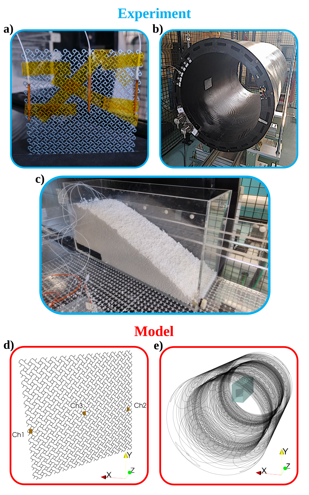
The measurements were conducted on a semi-rigid titanium (ASTM F67) cranial mesh manufactured by Medartis AG (Basel, Switzerland). The implant was 93 mm×93 mm and its thickness was 0.6 mm. The thickness of the implant corresponds to the diameter of its one-dimensional structure, so that r = 0.3 mm. It was equipped with three optical fibre temperature probes, two positioned in the peripheral regions, where the largest temperature increase was expected to be induced, and one in the central region, as shown in Fig. 2a. The probes were connected to an eight-channel AccuSens signal conditioner produced by Opsens (Qu´ebec, Canada) sampling at 20 Hz. The manufacturer declared an overall accuracy of ±0.30 ◦C and a resolution of 0.01 ◦C.

In a first experiment, simulating the heat transfer from the cranial mesh towards soft tissues, the implant with the positioned probes were plunged into a cuboid container (base of 13 cm × 44 cm, height of 20 cm) filled with gel simulating average tissue parameters produced by Zurich MedTech AG (Zurich, Switzerland) in accordance with ISO/TS 10974 . In a second experiment, simulating an almost adiabatic condition, the same cuboid container was filled with expanded polystyrene grains whose diameter varies between 1 mm and 3 mm (Fig. 2c). The base of the implant was fixed in a slot cut in a spongy support to keep it in the correct position within the container (see Fig. 2a).

In particular, the implant was positioned at 45◦with respect to the container walls to have it perpendicular to the generated magnetic field, which is the configuration expected to maximize the induced temperature increase.

The magnetic field was generated by the system of actively shielded GCs with whole-body access for cylindrical MRI scanners depicted in Fig. 2b. Precisely, it is the model Solaris-R manufactured by Nanjing Cichen Medical Technology Co., Ltd (Nanjing, China). The system, featuring three coils to generate gradient magnetic fields along three orthogonal directions, has an internal diameter of about 67 cm and a total length of about 150 cm. The gradient directions determine the used reference system illustrated in Fig. 2e, with ˆz directed longitudinally with respect to the coils, ˆy directed vertically and ˆx perpendicular to the other two directions.

The GCs were supplied by a NG500 1.3 gradient amplifier built by Prodrive Technologies (Eind- hoven, The Netherlands) able to drive each coil independently and to provide a peak current of 1000 A and a maximum voltage of 940 V. To dissipate the loss power in the coil conductors due to the high current values, a water cooling system was connected to the coils. The cooling system made negligible the impact of the heating dissipated by the GCs’ conductors on the temperature values measured on the implant, as verified through a fourth optical fibre temperature probe positioned at the boundary of the phantom, where no heating due to the currents induced on the cranial mesh was expected. In the experiment, the coils generating gradients directed along ˆx and ˆz were driven with two in-phase sinusoidal currents at the frequency of 2 kHz. According to the numerical model described in Section 2.2.2, the peak current intensities of 150 A were such that a peak magnetic field of 3.5 mT was generated at the implant barycentre, located at x = 14 cm, y = 0 and z = 30 cm with respect to the coil isocentre (i.e., the central point where all the coils generate a null magnetic field).

8

Figure 2: Experimental setup and virtual modelling. a) Semi-rigid cranial mesh in titanium equipped with the optical fibre temperature probes. b) System of GCs for cylindrical MRI scanners. c) Phantom filled with expanded polystyrene grains. d) Computational model of the cranial mesh with depicted the boxes of the active parts of the temperature probes. e) Computational domain including the phantom with the cranial mesh and the model of the GCs.

The temperature detected by the optical fibre temperature probes were recorded every 2 s for 900 s of continuous exposure of the cranial mesh to the harmonic magnetic field generated by the GCs. Temperature recording started 30 s before switching on the power amplifier to acquire the value at which the system and the probes were thermalised.

Since The Actual Measurand To Be

compared with the simulation results is the temperature increase, an offset equal to the average of the temperature values recorded in the preliminary 30 s were applied to the measurement results. The measurements were repeated two times a day apart without moving neither the probe nor the phantom, to assess the repeatability of the experiment.

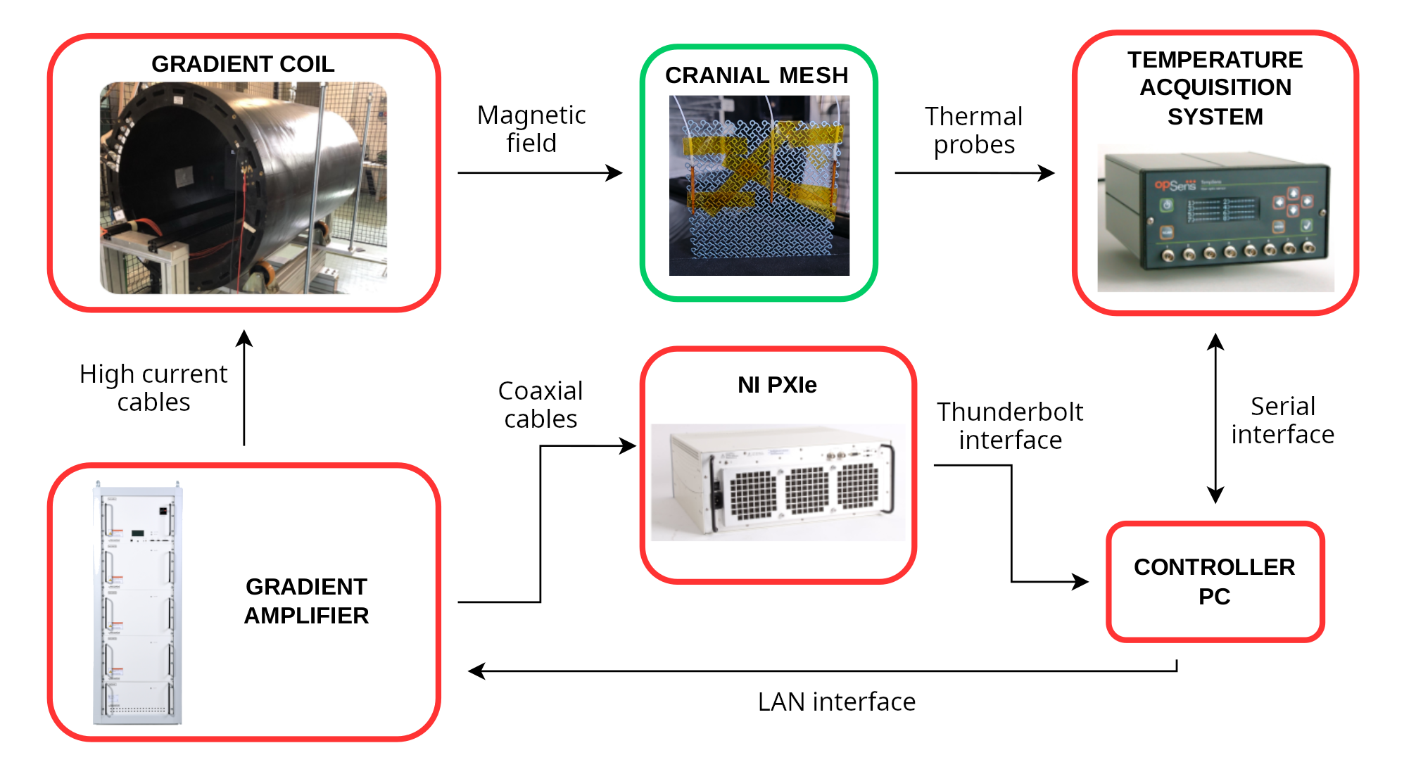
Figure 3 depicts the measurement pipeline. The temperature probes attached to the implant were connected to the temperature acquisition system, which transmitted the acquired temperature data to the controller PC through a serial interface. Meanwhile, the currents flowing into the GCs

9

Figure 3: Experiment pipeline. The experiment was monitored by a controller PC that collected the acquired temperature data through a serial connection with the temperature acquisition system. The same controller PC controlled the gradient amplifier through a LAN connection and moni- tored the generated currents through a Thunderbolt connection and an acquisition board connected through coaxial cables to the gradient amplifier. The gradient amplifier supplied the GCs through high current cables and the cranial mesh was exposed to the generated magnetic field.

were monitored through a 3-channel acquisition board connected to a National Instrument (Austin, Texas) PXIe. The current output monitor of the gradient amplifier were connected to the acquisition board with three coaxial cables and data from the acquisition board were transmitted to the PC through a Thunderbolt interface. The gradient waveform was set on the amplifier through a LAN interface controlled by the amplifier’s proprietary software installed on the controller PC.

Numerical Model

The one-dimensional model of the cranial mesh was created by repeating the elementary cell re- ported in Fig. 1c until a square of 93 mm sides was filled (see Fig. 2d). The entire implant geometry

Is Described By

about 8000 segments. The electrical currents induced in the implant were com- puted according to the method described in Section 2.1.1, considering an electrical conductivity of 1.82 MS m−1.

The application of the Biot-Savart law to a model of the gradient coils (depicted in Fig. 2e) allowed the computation of the magnetic vector potential along the model branches, providing the electromotive forces to the electrical network problem. The computed currents were processed according to (1) to evaluate the linear power density dissipated in the cranial mesh.

Table 1: Thermal properties of the materials involved in the experimental comparison.

Related Journal Articles & DOI Links

Selected peer-reviewed publications relevant to 12 Lead ECG Acquisition. Click the DOI to access the full paper (may require institutional access).

Why Choose Us?

Bangalore guidance for robotics, Spectre and autonomous systems projects.