Ansys Lead Extraction Force

Label-dependent Feature Extraction in Social Networks

For Node Classification

Tomasz Kajdanowicz1, Przemysław Kazienko1, Piotr Doskocz1 Abstract. A new method of feature extraction in the social network for within- network classification is proposed in the paper. The method provides new features calculated by combination of both: network structure information and class labels assigned to nodes. The influence of various features on classification performance has also been studied. The experiments on real- world data have shown that features created owing to the proposed method can lead to significant improvement of classification accuracy.

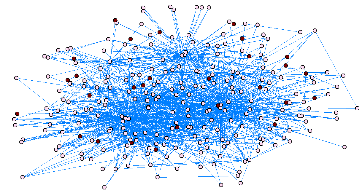
Keywords: feature extraction, label-dependent features, classification, social

1 Introduction

Classification is one of most important concepts in Machine Learning. It is usually based on the data that represents relationships between a fixed set of attributes and one target class. These relations describe each object independently that means no direct correlations between objects in the classification phase are taken into account.

An exception may be additional input features, which aggregate information about the entire group a given object belongs to. However, it requires any clustering process be launched before. There are some applications and research methods, especially related to social networks, which are able to produce data with dependencies between labels of interconnected objects, referred as relational autocorrelation . Based on these connections additional input information should be added to the classification process.

If the considered objects are humans and the classification is utilized on their profiles then the social network can be extracted from complementary data (different from people’s profiles) about common activities and mutual communication [9, 10, 15].

Overall, a social network is a set of nodes (human entities, objects) and node-node relationship between pairs of nodes . According to , all network objects may be described by three distinct types of information that can be easily used in label classification: correlation between the object’s label (class) and its attributes, correlation between the object’s label and the observed (known) labels of other objects in its neighborhood and, consequently, correlation between the object’s label and unobserved (unknown) labels of other objects in its neighborhood.

Basic task of within-network classification [1, 12] is to assign the correct labels to the unlabeled nodes from a set of the possible class labels. For example, based on the network of communication interactions, it could be determined whether a given company’s employee is either an executive or a performer. Willing to obtain the best possible results of classification, all three types of information should be evaluated: nodes attributes (profiles), node-node network relations to the known labels in the neighborhood (labeled neighbors) and relations to the neighboring objects with unknown labels. Main difficulty here is to extract the set of most discriminative features from the network nodes and their connections to achieve the best classification model.

A new approach for network feature extraction is proposed in further sections. Some of these structural features have discriminative distribution, which may directly influence classification performance.

Section 2 covers related work while in Section 3 appears main part of the paper, where a new method for network feature extraction is presented. Sections 4 and 5, contain descriptions of the experimental setup and the obtained results, respectively.

The paper is concluded in Section 6.

2 Related Work

In recent years, there has appeared a great number of works describing models and techniques for classification in network data. Analogously to classical machine learning problems, classification in network data requires specialized solutions for feature extraction, high performance supervised and unsupervised learning algorithms, sparse data handling, etc.

In general, network classification problems, may be solved using two main approaches: by within-network and across-network inference. Within-network classification, for which training entities are connected directly to entities, whose labels are to be classified, stays in contrast to across-network classification, where models learnt from one network are applied to another similar network . Overall, the networked data have several unique characteristics that simultaneously complicate and provide leverage to learning and classification. More generally, network data allow the use of the features of the node’s neighbors to label them, although it must be performed with care to avoid increase of variance estimation .

There have been developed many algorithms and models for classification in the network. Among others, statistical relational learning (SRL) techniques were introduced, including probabilistic relational models, relational Markov networks, and probabilistic entity-relationship models [2, 6, 13, 16]. Two distinct types of classification in networks may be distinguished: based on collection of local conditional classifiers and based on the classification stated as one global objective function. The most known implementations of the first approach are iterative classification (ICA) and Gibbs sampling algorithm (GS), whereas example of the latter are loopy belief propagation (LBP) and mean-field relaxation labeling (MF) . Generally speaking, there exist many pretty effective algorithms of collective classification as well as graph-based semi-supervised learning methods. It refers, especially logForest, a logistic model based on links, wvRN, a relational neighbor model, SSL Gaussian random field model, ghostEdge, combination of statistical relational learning and semi-supervised learning for sparse networks and theirs collective classification supplements .

One of the most crucial problems in the network classification is feature extraction. According to the derived features are divided into two categories: label-dependent (LD) and label-independent (LI). Features LD use both structure of the network as well as information about labels of the neighboring nodes labels, e.g. number of neighbors with given class label. Features LI, in turn, are calculated using the network structure only, e.g. betweenness of a node. The LI like features, therefore, are independent from the distribution of labels in the network and might not be informative. However, they can be perfectly calculated regardless of the availability of labels. What is worth mentioning, most of the proposed network classification methods were usually applied to the data sets with very limited access to labels. Their authors assumed that their applications need to deal even with only 1% labeled nodes.

This problem is known as classification in sparsely labeled networks [4, 5]. It appears that the majority of network-based structural measures used as features in network classification may be useful and may potentially improve classification performance.

Social networks, being a network representation of interactions between people is a subject of research in terms of classification in networks as well .

3.1 General Terms

Let us suppose that a social network is a graph G = (V, E, X, L, Y, W), where V is a set of nodes (objects, social entities); E is a set of edges (connections) eij between two nodes vi and vj, E={eij: vi,vjV, i≠j}; X is a set of attribute vectors xi, a separate one for each node vi (a profile of vi), X={xi: viVxiX}; L is the set of distinct labels (classes) possible to be assigned to nodes; Y is a list of actual labels assignments to nodes, Y={: viV  yiL}; W is a set of edge weights, wijW wij≥0 and wij indicates the strength of edge eij.

Having known the values of yi for a given subset of nodes VKV, classification may be described as the process of inferring the values of yi for the remaining set of nodes VU, VU = V \VK.

The first step in the process of node classification is a translation of network data into a set of unified vectors, one for each node. A single vector corresponding to node vi contains all information from xi as well as some additional information (new attributes) derived by feature extraction methods based on the network profile. Next, the obtained set of vectors is used in classical, supervised classification.

3.2 Features Extraction

Feature extraction from social networks is a general term for methods of constructing variables from the connectivity graph, expressing the position and importance of each node with respect to the others. As mentioned in Section 1, the generated features may be label-independent or label-dependent. For clarity, while describing label- dependent features, it is made a basic assumption in the paper that feature extraction is based only on correlation between the object’s label and the observed labels of other objects in its neighborhood see Fig. 1.

Fig. 1. Example social network with 10% of unlabeled nodes (black circles denote labeled nodes). Three examples of basic label-independent and three label-dependent features are presented in the following sub-sections, as well as generalization for label-dependent features extraction.

Betweennes Centrality

Betweenness centrality of node vi pinpoints to what extent vi is between other nodes. Nodes with high betweennes are very important in the network as other nodes are connected with each other mainly through them. Betweenness centrality B(G,vi) of node vi in graph G can be calculated according to the following equation:

Where:

P(G,vi,vj) - a function returning the number of shortest paths between vi and vj in

Graph G;

P(G,vj,vk,vi) - a function that returns the number of shortest paths between vi and vj that pass through vi in graph G. Obviously, Equation 1 is calculated only for pairs vj, vk, for which there exists a path from vj to vk to prevent the denominator from equaling 0.

Degree Centrality

Degree centrality is defined as the number of connections (edges) incident upon a given node. It is the simplest and most intuitive measures that can be used in the network analysis. Nodes with the high degree centrality are recognized as a crucial cog that occupies a central location in the network. Degree centrality D(G,vi) of node

Where:

n(G,vi) - a set of neighboring nodes of node vi in graph G.

Local Clustering Coefficient

The local clustering coefficient CC(G,vi) of a node vi in graph G quantifies how close vi‘s neighborhood is to a complete graph, see Equation 3.

Where:

R(V) - an operator returning the number of all connections between nodes from set V.

3.2.2 Label-Dependent Features

While introducing label-dependent features two manners of their formation are proposed. Both of them relay on the idea of selective definition of sub-networks based on the labels assigned to each node. It means that a sub-network for a given label l consists of only those nodes that share label (class) l together with all edges connecting these selected nodes. For that purpose, a new selection operator O(G,l) for graph G and label l is defined. It returns a sub-network Gl labeled with l: Gl=(Vl, El,

Yl={: ViVYl=L},

El={eij: vi,vjVleijE}, Xl={xl: vlVlxlX}. Afterwards, for each sub-network Gl (each label l), new features are computed. First group of label-dependent features composition is based on new custom measures derived from the interaction between a given node and its neighboring nodes only.

The measures take into consideration either the number of connections or their strengths. Normalized Number of Connections to the Labeled neighbors The measure for the normalized number of connections to the labeled neighbors NCN(G,l,vi) represents the proportion of the number of connections to the neighboring nodes in the sub-network with label l (Gl) by the number of connections to the labeled neighbors in the whole primary graph G (with all labels).

Where:

n(O(G,l),vi) - a set of the neighboring nodes for node vi in sub-network O(G,l), nL(G,vi) - a set of vi‘s labeled neighbors in graph G, each neighbor must be labeled with any label lL.

Note that the value of card(n(O(G,l),vi)) is the same as the number of connections between vi and vi’s neighbors (each vi’s neighbor has one connection with vi). Similarly, the value of card(nL(G,vi)) equals the number of connections between vi and all vi’s labeled (and only labeled) neighbors.

The measure NCN(G,l,vi) is computed separately for each label l and in general, for two labels lk and lm, the value of NCN(G,lk,vi) may differ from NCN(G,lm,vi). For the example network from Fig. 2, and the measure NCN(G,’red’,v1) calculated for node 1 in the sub-network with nodes labeled with the ‘red’ class, the value of NCN(G,’red’,v1) is 4 divided by 8 (total number of nodes in graph G).

W15

Fig. 2. Feature calculation based on label dependent neighborhood. For each of label class {white, red} w is calculated. Normalized Sum of Connection Strengths to the Labeled Neighbors The value of the normalized sum of connection strengths to the labeled neighbors NCS(G,l,vi) is the proportion of node vi’s activity towards vi’s neighbors (measured by the aggregated connection strengths) in the sub-network with label l (Gl) normalized by the equivalent value of strengths to the neighbors with any label in the whole graph G. The value of NCS(G,l,vi) for graph G and label l is expressed in the following way:

(5)

Similarly to NCN(G,l,vi), the measure NCS(G,l,vi) is evaluated separately for each label l and differs for different labels l. For the network from Fig. 2, the measure NCS(G,’red’,v1) is computed for node 1 and label (class) ‘red’, as the sum of w13, w14, w17, and w18 normalized by sum of all eight connection strengths.

3.2.3 General Method for Label-dependent Features Extraction In the domain of social network analysis (SNA), a number of measures characterizing network nodes have been introduced in the literature. Majority of them is label- independent and it is possible to define many methods that will extract label- dependent features based on them. A general concept of creation of any label- dependent feature Ml(G,l,vi) for label l and node vi in the social network G applies label-independent feature M to the appropriate labeled sub-network Gl=O(G,l), as

Where:

Ml(Gl,vi) - denotes any structural network measure for node vi applied to sub-network Gl=O(G,l), e.g degree, betweennes or clustering coefficient; Obviously, Ml(G,l,vi) is computed separately for each label l using the appropriate sub-network Gl=O(G,l). In other words, Eq. 6 provides a method for construction of label-dependent version of certain metric.

As an example, the label-dependent clustering coefficient (CCl) is defined in

4.1 Data Set

The data set used for experiments, “Attendee Meta-Data” (AMD), was downloaded

(Http://Networkdata.Ics.Uci.Edu/

data.php?d=amdhope). The AMD data set was an output of a project, which used RFID (Radio Frequency Identification) technology to help connect conference participants at “The Last HOPE” Conference held in July 18-20, 2008, New York City, USA. All attendees received an RFID badges that uniquely identified and tracked them across the conference space. The data set contains descriptions of

Related Journal Articles & DOI Links

Selected peer-reviewed publications relevant to 12 Lead ECG Acquisition. Click the DOI to access the full paper (may require institutional access).

Why Choose Us?

Bangalore guidance for robotics, Spectre and autonomous systems projects.