Comsol Infusion Set Flow

1

Scientific Reports | (2020) 10:10102 | https://doi.org/10.1038/s41598-020-66887-w

Pumping

Ravi Teja Kedarasetti1,2, Patrick J. Drew1,2,3,4 & Francesco Costanzo1,2,3,5 ✉ The brain lacks a traditional lymphatic system for metabolite clearance. The existence of a “glymphatic system” where metabolites are removed from the brain’s extracellular space by convective exchange between interstitial fluid (ISF) and cerebrospinal fluid (CSF) along the paravascular spaces (PVS) around cerebral blood vessels has been controversial. While recent work has shown clear evidence of directional flow of CSF in the PVS in anesthetized mice, the driving force for the observed fluid flow remains elusive. The heartbeat-driven peristaltic pulsation of arteries has been proposed as a probable driver of directed CSF flow. In this study, we use rigorous fluid dynamic simulations to provide a physical interpretation for peristaltic pumping of fluids. Our simulations match the experimental results and show that arterial pulsations only drive oscillatory motion of CSF in the PVS. The observed directional CSF flow can be explained by naturally occurring and/or experimenter-generated pressure differences.

The flow of cerebrospinal fluid (CSF) in the brain is hypothesized to play an important role in the clearance of metabolic waste and maintenance of the ionic environment1–3. Recent work suggests that the paravascular spaces (PVS) surrounding cerebral arteries provide a low-resistance pathway for the bulk flow of CSF into the brain1,4–7. However, this idea that there is bulk fluid movement into the brain is highly controversial, with both simulations8–10 and experiments6,7,11,12 being put forward both in support of and against bulk flow. One of the leading theories in support of bulk flow in the PVS identifies “peristaltic pumping” as the flow driver, i.e., the idea that heartbeat-driven pulsations pump CSF in the PVS. Peristaltic pumping in a deformable tube is achieved by repeated contractions and dilations propagating along the wall of the tube. In fluid dynamics, peristaltic pump- ing is a well-understood mechanism of fluid transport. The mechanism of peristaltic pumping of fluids was first demonstrated by Latham13. Further work on the peristaltic pumping of fluids has encompassed a wide range of scenarios14–17. Calculations made using fluid dynamic principles can make very accurate predictions of fluid flow under peristalsis, and have been used in designing artificial peristaltic pumps18–20.

Recent work by Mestre et al.7 and Bedussi et al.6 used in vivo two-photon microscopy21 to simultaneously measure arterial pulsations and the flow of CSF in the PVS around the middle cerebral artery (MCA) by tracking the motion of fluorescent microspheres. They found that movement of CSF in the PVS had two components, a constant flow in the direction of blood flow with an average velocity of approximately 20 µm/sec, and an oscilla- tory flow in phase with the arterial pulsations6,7, with a peak velocity of approximately 10 µm/sec. Based on these observations, it has been proposed that peristaltic motion of the arterial wall generates a “pumping” force that drives the net flow of CSF parallel to the direction of the pulse wave propagation.

In this study, we apply the well-established fluid dynamic principles of peristalsis to study the nature of fluid flow in the PVS, aiming to bridge the gap between experimental observations and hypotheses. As previous stud- ies of CSF flow in the PVS disagree on both the direction and the flow rates8–10, we started our calculations by revisiting the mechanism of peristaltic pumping using time-dependent fluid dynamic simulations with fluid particle tracking in a deforming domain. By emphasizing the mechanism of peristatic pumping, we aimed at providing a clear physical interpretation for our calculations. We then performed fluid dynamic simulations on more realistic models of the PVS. Our simulations suggest that peristalsis with physiologically-plausible pulsation cannot drive the experimentally-observed fluid flow. However, we found that a small, constant pressure gradient

2

Scientific Reports | (2020) 10:10102 | https://doi.org/10.1038/s41598-020-66887-w

Www.Nature.Com/Scientificreports/

(of order 0.01 mmHg/mm) can account for the net forward movement observed experimentally. These results suggest that the observed directional movement of CSF in the PVS is generated by naturally occurring and/or experimenter-generated pressure differences, but not by arterial pulsations.

Results

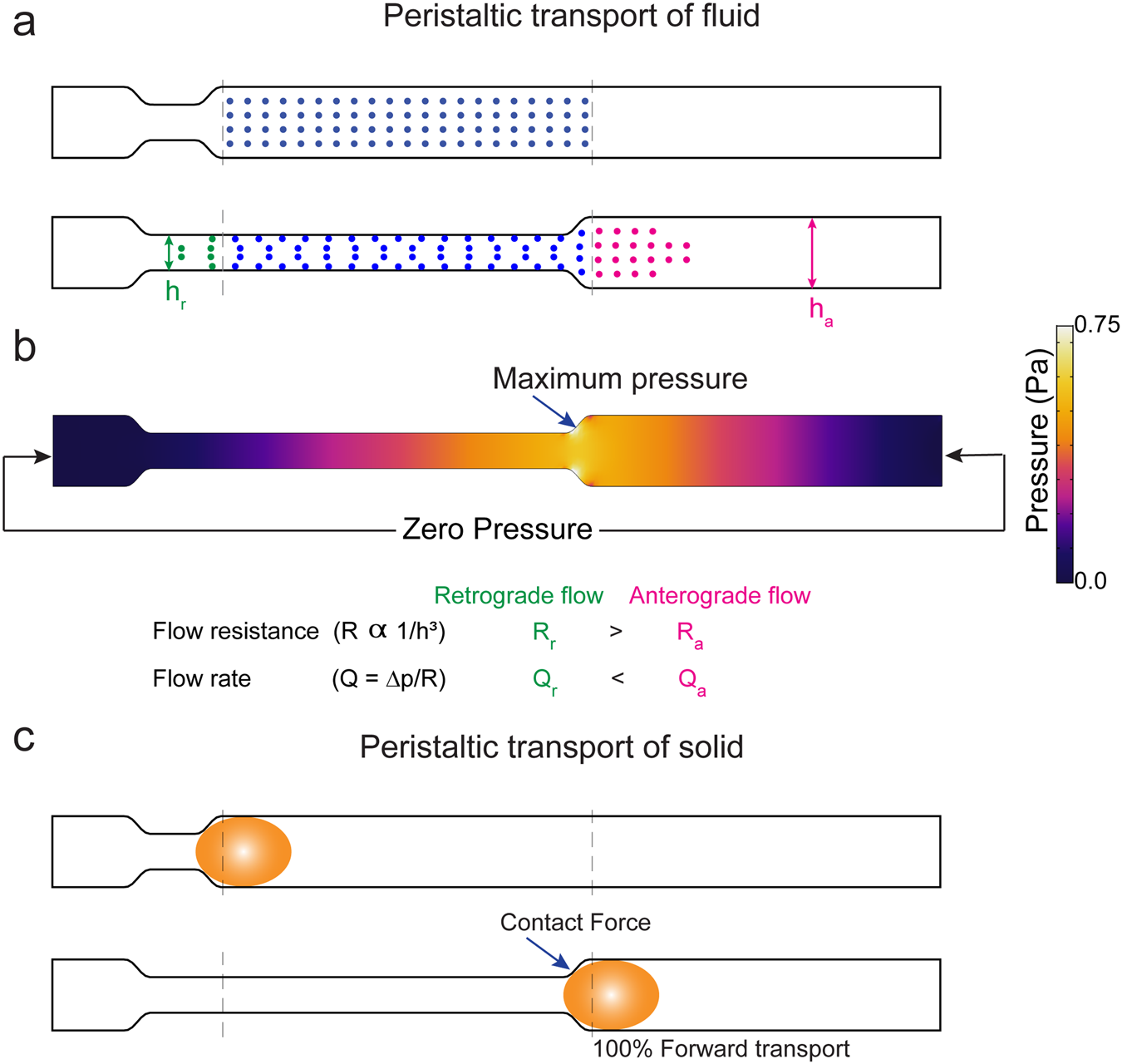
We first examine how peristaltic motion affects the flow of an incompressible fluid in a two-dimensional tube. Consider a fluid-filled tube with deformable walls and no pressure difference across its two ends. When the posi- tion of the walls is fixed, there is no pressure gradient, and therefore no fluid flow (Fig. 1a,b). When the walls move inward due to a peristaltic wave propagating to the right (Fig. 1a), the fluid-filled domain deforms and the fluid is displaced. When the direction of the fluid flow is the same as the peristaltic wave, the motion is said to be anterograde – otherwise it is said to be retrograde. The flow in both directions is a result of the fluid pressure distribution, shown in Fig. 1b. The pressure is maximum at the location of the moving neck and is minimum at the two ends of the tube. Therefore, the fluid that is displaced by the wall is subject to the same pressure difference

A

r, where the subscripts ‘a’ and ‘r’ denote the anterograde and retrograde flows, respectively). However, since the width of the tube (h) is smaller in one direction (

R), There Is More Resist-

ance for retrograde flow than anterograde flow (since flow resistance R scales with width of the tube

A

r). As a result of this difference in flow resistance, the anterograde flow is greater than the retro-

A

r). Thus, while peristalsis drives both anterograde and retrograde flows, a net flow in the direction of the peristaltic wave emerges (Video SV1). This example is a simplified version of peristalsis, where, the walls of the fluid-filled tube only contract. An example with a periodic contraction and expansion of the walls is demonstrated in Fig. S1 and Video SV2.

Figure 1.  Mechanism of forward transport (pumping) driven by peristalsis in fluids and solids. (a) The movement of fluid (the dots represent fluid particles) driven by peristaltic compression of the walls of a 2D tube. The fluid movement in this figure is calculated using the Navier-Stokes equation with zero traction (pressure) at the two ends of the tube. (b) The pressure field in the tube in the deformed state. The fluid is displaced by the moving walls and this creates high pressure at the neck of wall movement. The pressure difference is same for retrograde and anterograde flow. However, the resistance is large posterior to the site of contraction. Compared to anterograde flow, retrograde flow needs the fluid to flow through a narrower tube. This results in a greater anterograde flow (magenta dots in a) compared to retrograde flow (green dots in a). (c) The movement of a solid bolus (yellow ellipse) driven by peristaltic motion of the walls of a 2D tube. The contact forces between the moving walls and the solid bolus are responsible for forward transport. The position of the solid bolus with respect to the dotted lines shows that the solid is moved forward. (a) was generated with MATLAB 2019b(https://www.mathworks.com/ products/matlab.html). (b) was generated with COMSOL Multiphysics 5.4 (http://comsol.com). (c) was drawn in Adobe Illustrator 23.0(https://www.adobe.com/products/illustrator.html).

3

Scientific Reports | (2020) 10:10102 | https://doi.org/10.1038/s41598-020-66887-w

Www.Nature.Com/Scientificreports/

It is important to bear in mind the difference between peristaltic transport of fluids and peristatic transport of solids. The textbook picture of peristalsis22,23 is derived from the transport of solid matter in the esophagus and the gastro-intestinal tract. When solid matter is transported by peristalsis, all of the material moves in the direc- tion of the peristaltic wave (Fig. 1c). This differs from the case of fluid transport by peristalsis, which generates both anterograde and retrograde flows (Figs. 1b, S1). Moreover, the peristaltic transport of solids is independent of the magnitude of wall motion and the length of the tube. In contrast, the nature of fluid flow in a tube driven by peristaltic motion of the walls is highly depended on the magnitude of both wall motion and tube length24, which we will demonstrate in the results. This understanding of the mechanism of peristaltic transport of fluids is crucial to interpreting the results of fluid dynamic models of the PVS. The assumptions of the shape, size and the defor- mation of the PVS may vary between the models, but the mechanism of peristaltic transport remains the same.

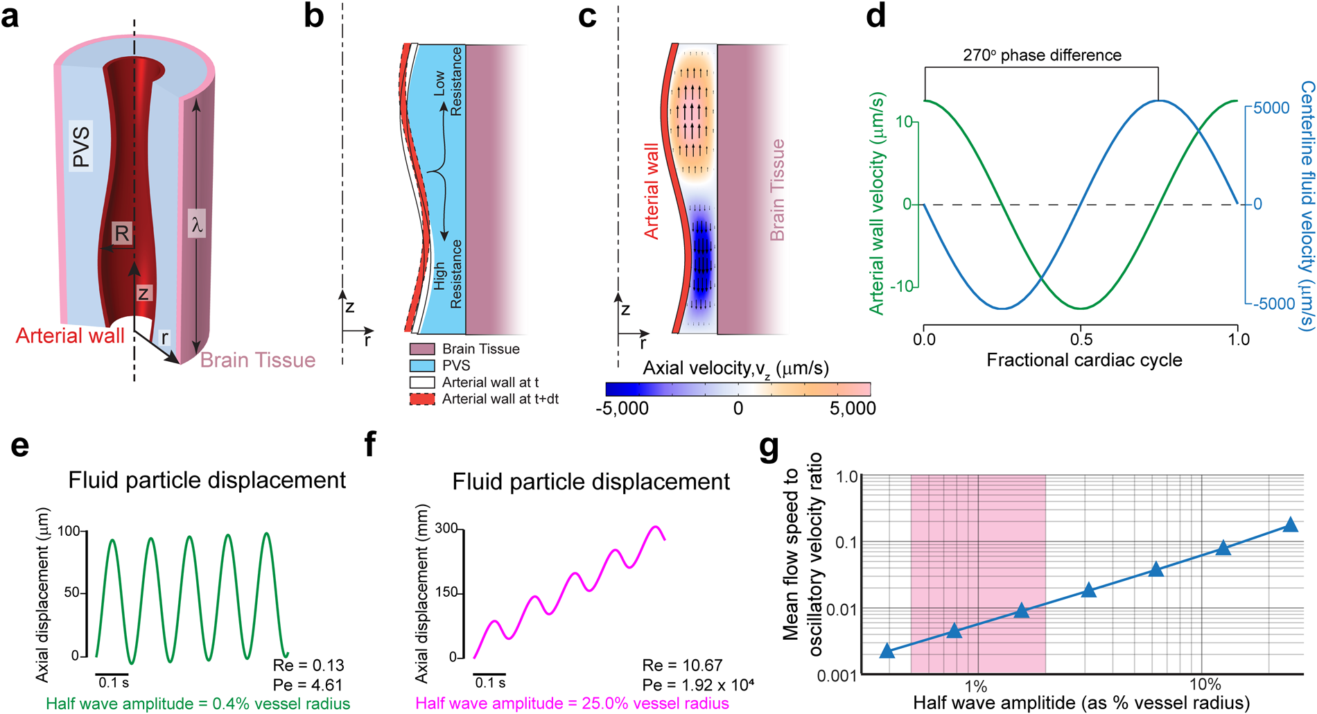
Peristaltic pumping requires unphysiologically large amplitude pulsations for meaningful fluid flows. To understand the relation between arterial wall movement and fluid movement in the PVS, we created a model of peristaltic pumping. In our model, the geometry of the PVS is taken to be cylindrically symmetric, with the artery centered within the PVS (Fig. 2a). While the geometry of the fluid domain is simplified, the inner and outer radii are based on realistic values (see methods). We then imposed a sinusoidal peristaltic wave on the arterial wall, while keeping the outer wall of the PVS fixed, effectively making the brain tissue rigid. In order to capture the whole peristaltic wave, the length of the PVS used in the simulation was equal to one wavelength (λ) Figure 2.  Heartrate pulsations drive oscillatory, but not directional flow. Large non-physiological pulsations are required for appreciable peristaltic pumping. (a) Schematic of the axisymmetric peristatic pumping model. The arterial wall undergoes peristatic movement, while the outer wall of the PVS is fixed. The length of the PVS is taken as one wavelength of the peristaltic wave (λ) with periodic boundary conditions at the two axial ends. (b) Schematic of the fluid motion during periodic peristalsis. The fluid displaced by the moving wall should move with lower resistance along the direction of the peristaltic wave than in the opposite direction. This difference in flow resistance results in net forward pumping. (c) The magnitude of the axial velocity is denoted by color, with arrows showing the direction. The half-wave amplitude of the peristaltic wave is 0.8% of the vessel radius.

The deformations are scaled by a factor of 50 in the figure to clearly show the arterial wall movement. (d) The plots show the relative phase between arterial wall velocity and the centerline fluid velocity at the same axial (z) location (midpoint, z = λ/2). There is a 270° phase difference between the wall velocity and fluid velocity.

(e) The trajectory (in z) of a fluid particle at the center of the PVS, where the amplitude of the peristaltic wave is similar to heartbeat driven pulsation6,7 (0.8% peak-to-peak change in arterial radius). The flow is mostly oscillatory with very little unidirectional movement. (f) The trajectory (in z) of a fluid particle at the center of the PVS, where the amplitude of the peristaltic wave is unrealistically large (50% peak-to-peak change in arterial radius). This trajectory with appreciable unidirectional movement looks similar to experimental results6,7. (g) Plot showing the ratio of mean flow speed (average unidirectional flow velocity) to oscillatory velocity (peak velocity change in a cycle) as a function of the amplitude of the peristaltic wave. The shaded region shows the normal amplitude of pulsation cerebral arteries (1–4% of arterial radius peak-to-peak). Note that in this range, the oscillatory velocity is ~2 orders of magnitude higher than the pumping velocity (a–d). were generated with COMSOL Multiphysics 5.4(http://comsol.com). (e–g) were generated with MATLAB 2019b(https://www.

mathworks.com/products/matlab.html).

4

Scientific Reports | (2020) 10:10102 | https://doi.org/10.1038/s41598-020-66887-w

Www.Nature.Com/Scientificreports/

of the peristaltic wave (see methods). Since we are interested in studying the pumping generated by arterial wall movement alone, we used periodic boundary conditions at the axial ends of the PVS. This is equivalent to stud- ying flow driven by peristalsis with no additional pressure differences8,14,15,25. We tracked the motion of particles at the center of the PVS.

Peristaltic pumping of fluid is a result of lower flow resistance for anterograde flow and higher resistance for retrograde flow (see Figs. 1 and 2b). This explains the fluid velocities observed with respect to the arterial wall position and wall velocity (Fig. 2c,d). The phase difference between the arterial wall velocity and the downstream fluid velocity (axial velocity, vz) remained the same throughout the length of the domain. Flow resistance (

Rflow

of a tube with an annular cross-section decreases with approximately the fourth power of the internal radius26. For slow, laminar flows like those in the paravascular space, the flow resistance of a tube with annular cross-section is

1

1

Where Q is the flow rate, p is the pressure and µ is the dynamic viscosity of the fluid. The internal and external radii of the annular region are given by r1 and r2 respectively. For our calculations, Reynolds numbers range from 0.13 to 10.67, well within the laminar flow regime. Given the strong dependence of fluid resistance on the diame- ter, it follows that the amplitude of pulsations (the change in internal radius) should have a large effect on the flow resistance changes and therefore the pumping generated by peristaltic motion.

We examined the relation between pulsation amplitude and the trajectory of the fluid particles in the PVS. To put our results in the context of experimental findings, the typical half wave amplitude of heartbeat pulsations is 0.5–2% of arterial diameter6,7. Our simulations show that such small amplitude pulsations generate little differ- ence between forward and backward flow resistance, which resulted in oscillatory fluid flow with minimal net anterograde flow (Fig. 2e). However, the kind of fluid particle trajectories reported by Bedussi et al.6 and Mestre et al.7 are very different from the ones simulated in Fig. 2e. The fluid trajectories in the PVS observed in both studies are more similar to the ones shown in Fig. 2f, where the net anterograde motion of the fluid is of the same order as the oscillatory motion. Sample CSF particles trajectories can be found in the supplementary videos of Mestre et al.7 and Fig. 3 of Bedussi et al.6. This kind of fluid motion would require non-physiological amplitudes arterial pulsations, with half wave amplitudes around 25% of the arterial radius. To better understand the effect of pul- sation amplitude on fluid flow, we examined the relation between the pulsation amplitude and the ratio of mean flow speed (or average anterograde velocity) to oscillatory velocity (difference between peak anterograde velocity to peak retrograde velocity) (Fig. 2g). Measurements by Mestre et al.7 show that mean flow speed (~20 µm/s) and oscillatory velocity (~10 µm/s) are of the same order. Our simulations show that for heartbeat-driven pulsations (1–4% of arterial radius peak-to-peak6,7,27), the mean flow speed is 2–3 orders of magnitude smaller than the oscillatory velocity (Fig. 2g). These result show that heartbeat-driven pulsations in an idealized model are too small to explain the directed flow of CSF seen in vivo.

While the shape of the PVS in our model was simplified, the model still provides important generalizable insights into the mechanism of peristalsis. Specifically, the model helps us understand the relation between the movement of the arterial wall and the flow of fluid. We found that the radial wall velocity and the anterograde fluid velocity are always out of phase (by 270°, Fig. 2c,d), and that the kind of fluid trajectories observed in vivo would require large, non-physiological amplitudes for arterial pulsations. Next, we examined if these results held for a 3-dimensional model of peristalsis with a realistically shaped PVS and pulse waveform.

Paravascular flow measurements are inconsistent with peristaltic pumping.

To Test If Fluid Flow

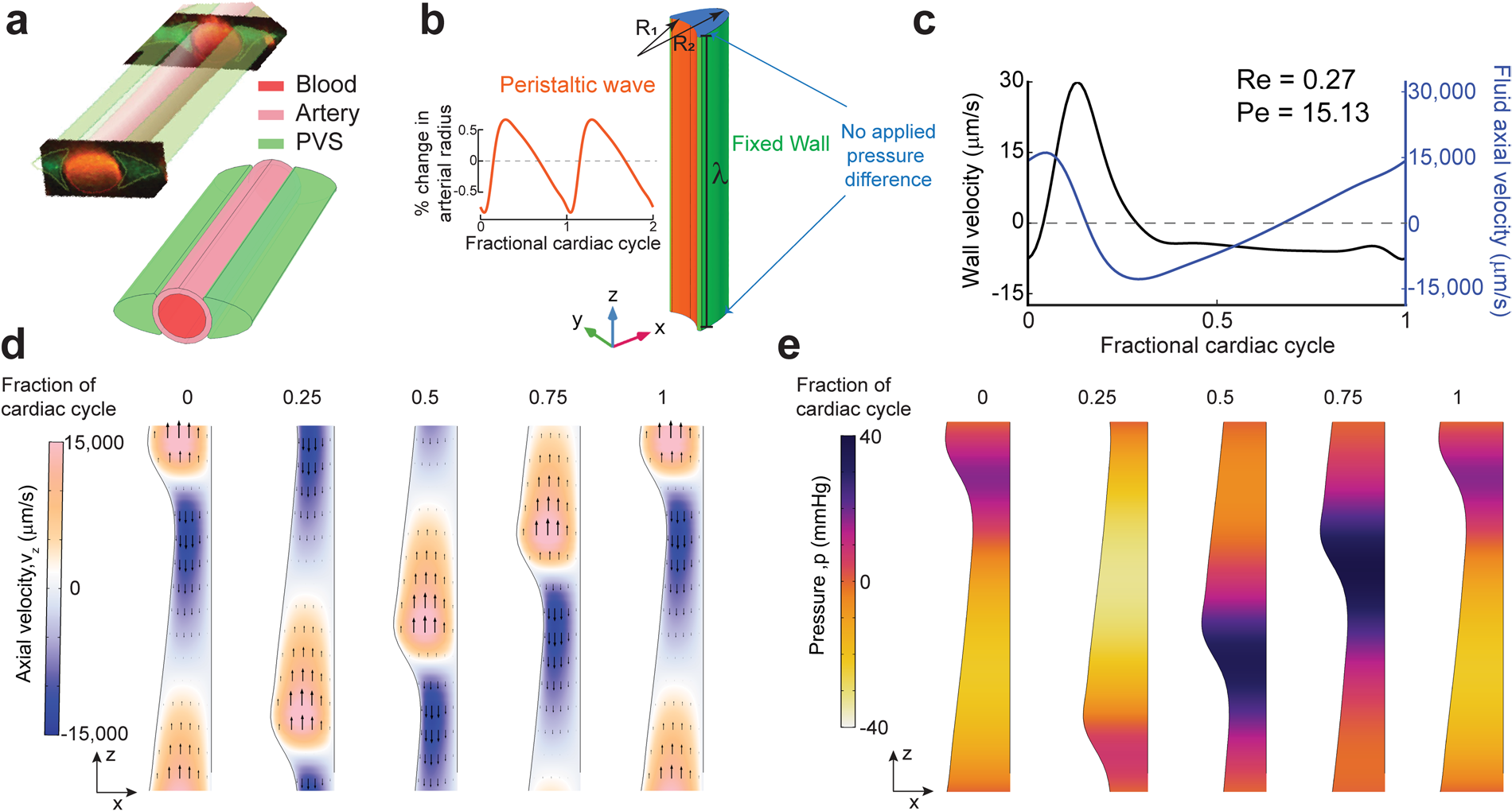
is influenced by the details of the shape of the PVS or the waveform of heartbeat driven pulsations, we created a model with a realistically-sized and shaped PVS, with a cardiac waveform drawn from experimental data7 (Fig. 3a,b). The outer wall of the PVS was assumed to be fixed, and the length of the domain was set to be equal to one wavelength (λ) of the peristaltic wave. We use a no pressure (traction) boundary condition at the boundaries in place of the periodic boundary condition used for the axisymmetric simulations. This is done to better estimate the pressure changes in the PVS (Fig. 3e).

The mean flow speed (anterograde velocity time-averaged over a complete cycle) of fluid particles at the centerline of the PVS in our simulation was 102.1 µm/s. However, this was accompanied by oscillatory fluid veloc- ities of approximately 30,000 µm/sec, well over a hundred times the mean flow speed (Fig. 3c,d). The simulations also show the phase relation between the arterial wall velocity (radial component of wall velocity) and the fluid anterograde velocity (axial component of fluid velocity). It is clear that the wall velocity and the fluid velocity are out of phase, i.e., when the arterial wall dilates, the fluid flows in the retrograde direction and, when the arterial wall constricts, the fluid flows in the retrograde direction. This phase relation between the velocities is consistent with our axisymmetric model (Fig. 2d). This is in contrast to the in vivo measurements by both Bedussi et al.6 and Mestre et al.7 (Fig. 4d), where the fluid flows in phase with the arterial wall, i.e., when the artery dilates, the fluid flow is anterograde and vice versa. Viewed together with the results of the axisymmetric simulations, our simu- lations suggest that the shape of the PVS and the waveform of heartbeat pulsations cannot pump CSF in a model with a simplified geometry of the PVS.

These results show that a peristaltic pumping model is inconsistent with experimental findings, which sug- gests that there are some problems with the assumptions of the peristaltic pumping model. In the next section, we revisit these assumptions and attempt to match the results of the fluid dynamic calculations with experimental findings.

5

Scientific Reports | (2020) 10:10102 | https://doi.org/10.1038/s41598-020-66887-w

Www.Nature.Com/Scientificreports/

Pressure differences, not arterial pulsations drive bulk fluid flow.

In Order To Better Capture The

geometry of the PVS, we made changes to our 3D model based on the anatomy of the brain, the subarachnoid space and cerebral vasculature. We shortened the length of the PVS to 5 mm, and made the outer wall of the PVS move with the pulsations. Previous peristaltic pumping models8,9,14,15 have set the length of the fluid chamber to be equal to one wavelength of the peristaltic wave. However, the wavelength of the peristaltic motion of arteries is considerably larger than the length of the middle cerebral artery (MCA), the proposed source of peristaltic Figure 3.  Simulations of arterial pulsations in a model with an elliptic PVS show that observed fluid flows are inconsistent with a peristaltic pumping mechanism. (a) The 3D geometry of the PVS used in our simulations replicates the PVS geometry observed in vivo in mice. The figure in top-left is taken from Mestre et al.7 and the figure on the bottom-right shows the 3D geometry used in our calculations. (b) The dimensions and boundary conditions used in 3D fluid dynamics simulations. The wall movement on the arterial side (orange) is given by a travelling wave with a realistic waveform observed in vivo in mice7 (inset). The wall on the brain tissue side is fixed (green). The parameters (R1, R2, λetc are given in Table 1). (c) Plots showing the arterial wall velocity and the centerline velocity of the fluid taken at the same axial (z) location. While the wall velocity profile and magnitude are very similar to what was observed in vivo7, the oscillatory fluid velocity is ~1000x higher than the values observed in vivo6,7. Moreover, the peak fluid velocity is not in phase with the wall velocity. These discrepancies were predicted by our simplified model (Fig. 2). (d) The colors show axial velocity profile at the mid-section of the PVS (XZ plane at y = 0) throughout the cardiac cycle. Arrows are provided to make the interpretation of flow easier. The fluid velocity profile agrees with our expectations from the mechanism of peristalsis (Fig. 2b) and our simplified model (Fig. 2c). The deformations are increased by a factor of 50 in post- processing to clearly show the arterial wall movement. (e) Corresponding pressure profile at the mid-section of the PVS (XZ plane at y = 0) throughout the cardiac cycle. The deformations are scaled by a factor of 50 in post-processing to clearly show the arterial wall movement. All the subplots were generated with COMSOL Multiphysics 5.4(http://comsol.com), with the exception of the top left image in a (citation provided).

81,82

Table 1.  Parameters used in simulations.

6

Scientific Reports | (2020) 10:10102 | https://doi.org/10.1038/s41598-020-66887-w

Www.Nature.Com/Scientificreports/

pumping. With a peristaltic wave speed of 0.5–2 m/s27,28, and a heartbeat frequency of 6–10 beats/second in mice6,7,29–31, the wavelength of the peristaltic wave is between 50–160 mm in mice, while the MCA is only 4–6 mm long in mice6,32,33. This means that the pulse wave travels so fast across the length of the PVS that the arterial wall moves in and out simultaneously and therefore there is no appreciable difference in the flow resistance for anter- ograde and retrograde flows (Fig. S2). We calculated the fluid particle trajectories 1 mm from the distal end of the PVS segment (z = 4 mm), which captures the geometry of the surface of the brain where the flow measurements were made. This corrected the inconsistency between the phase of the fluid downstream velocity and the arterial wall velocity found in the peristaltic pumping model with a length of one pulsation wavelength (Fig. S2). Our results are similar to the phase relation between arterial wall velocity and fluid velocity estimated by Asgari et al.10, who studied the flow driven by penetrating arterioles in a model with anatomically realistic dimensions.

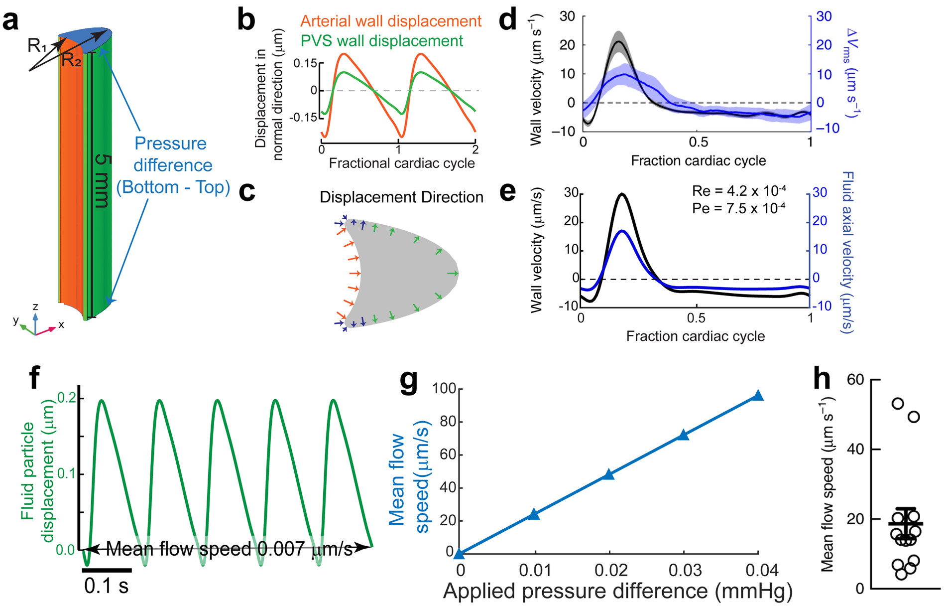
Secondly, the fixing of the outer wall of the PVS in other models means that the brain tissue and the subarach- noid space that surround the PVS are rigid. This is not realistic because the brain tissue is very soft, with a shear modulus in the range of 1–8 kPa34–38 (7.5–60 mmHg) and the 80 mmHg pressure changes (Fig. 3e) predicted by the peristaltic pumping model will cause substantial deformations. To include the effect of the soft tissue, we moved outer wall of the PVS with the same frequency as the heartbeat driven pulsations (Fig. 4b). We applied these small, pressure-driven deformations in the direction of the outward normal of the surface of the PVS, because pressure-like forces act along the outward normal of a surface. Since the mechanical properties of the Figure 4.  A small, constant pressure gradient can explain directed fluid movement in vivo. (a) Schematic of the model. The length of the PVS is set to 5 mm to match the length of the MCA in mice (4–6mm6,32,33). An additional pressure difference between the inlet and outlet is applied. (b) The displacement of the arterial wall (orange) and the PVS wall (green) used in the simulation. The displacement is given in the direction of the surface normals shown in (c). (c) Positive displacement direction at a cross-section of the PVS, this is the direction of displacement for the plots shown in (b) The Inner wall is shown in orange and the outer wall is shown in green. The displacement changes in amplitude and direction from the inner wall to the outer wall. This transition is carried out using the smooth, step function in COMSOL Multiphysics. The changing direction and length of the blue arrows indicates the smooth transition. (d) Plot showing arterial wall velocity and oscillations in fluid velocity measured in vivo. Adapted from Mestre et al.7 (e) Plot showing arterial wall velocity and oscillations in downstream fluid velocity our simulation matches with those in (d). (f) Plot of the trajectory of a fluid particle in the z direction shows that there is very little pumping by arterial wall movement.

(g) Plot showing the relation between an applied pressure difference across the ends of the PVS and the mean anterograde flow speed. An additional 0.01 mmHg pressure difference across the PVS is required to achieve a mean flow speed of 24.4 μm/s, similar to the mean flow speeds observed in vivo (h). (h) Mean flow speed in the PVS measured in vivo. Adapted from Mestre et al.7 (a–c,e). were generated with COMSOL Multiphysics 5.4 (http://comsol.com). (f,g) were generated using MATLAB 2019b (https://www.mathworks.com/products/ matlab.html).

Related Journal Articles & DOI Links

Selected peer-reviewed publications relevant to 12 Lead ECG Acquisition. Click the DOI to access the full paper (may require institutional access).

Why Choose Us?

Bangalore guidance for robotics, Spectre and autonomous systems projects.