COMSOL Ligament Stress Analysis

Biomechanical Behaviour of Soft Tissues — Ligaments & Tendons

Typical soft tissues include arteries and veins, cartilage, ligaments, tendons, muscles and skin. They are composite materials formed by an organic matrix reinforced by highly flexible collagen and elastin fibres with a high content of water.

Tensile-strength specialised tissues such as tendons and ligaments are rich in highly oriented fibres that essentially coincide with the direction of stress to which they are subjected and are therefore highly anisotropic. The organisation of tendons shows a hierarchical structure with fibres aligned along a preferential direction, whereas in veins and arteries two fibre families exist with helical orientation at opposite angles (providing circumferential rigidity against internal pressure).

Hierarchical structure (tendon / ligament)

• Collagen molecules → rod-like units aligned end-to-end in a staggered array
• Fibrils — smallest structural unit; diameters typically 10–500 nm (species, age and location dependent)
• Fibres — bound by endotenon (thin connective tissue with vessels and nerves)
• Fascicles — fibre bundles enclosed by the epitenon
• Tendon / ligament unit — surrounded by paratenon

This hierarchy provides the high tensile strength of tendons and ligaments. Because of the complexity of ultra- and microstructures, mechanical behaviour is commonly described with phenomenological models within elasticity, viscoelasticity or mixture theory frameworks under conditions of practical interest.

Source: Doblaré M., Merodio J. — An Introduction to Biomechanics and Mechanobiology (soft tissue section).

Typical Stress–Strain Curve for Tendons and Ligaments

A characteristic soft tissue stress–strain curve (e.g. tendon / ligament) has:

• Toe region (≈ up to 2% strain) — stretching-out of the crimp pattern of the composing fibres
• Linear region (≈ < 4% strain) — collagen fibres lose their crimp; slope is referred to as the Young modulus of the tendon. Deformations of soft tissues can be of the order of 100% in other regimes
• Microscopic tearing — beyond ≈ 4% strain
• Macroscopic failure / rupture — beyond ≈ 8–10% strain

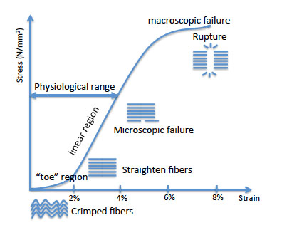
Figure: Typical stress–strain curve for tendons and ligaments (toe region → linear region → microscopic failure → macroscopic rupture). Adapted from biomechanics literature (Doblaré & Merodio).

Soft tissues are usually modelled as hyperelastic, quasi-incompressible and transversely isotropic materials subjected to large strains. Many early strain-energy density functions (SEDF) followed rubber-like isotropic forms \(W = W(I_C, II_C)\). A widely used family for fibre-reinforced soft tissue is transversely isotropic: \(W = W(I_C, IV_C)\) with \(IV_C = \mathbf{M}:\mathbf{C}\) and \(\mathbf{M} = \mathbf{a}\otimes\mathbf{a}\) the structural tensor of preferred fibre direction \(\mathbf{a}\).

Constitutive Modelling & Residual Prestress

Initial reference (zero-stress) state: Most soft tissues are under pretension in vivo to provide stability in the absence of external loads (as in ligaments) or to reduce circumferential stress gradients (e.g. arterial wall). Including residual stresses is essential for realistic kinematics and homeostasis predictions, but requires careful numerical formulation and experimental calibration.

Viscoelasticity: Internal friction between fibres, matrix and fluid induces viscoelastic behaviour that is especially important under cyclic loads or long-term strain (relaxation), as in physiological ligaments and after replacement with prestressed grafts. At low strain rates, tendons/ligaments are more deformable and absorb more energy but transfer loads less effectively; at high strain rates they become stiffer and more effective at load transfer.

Standard linear viscoelasticity is generally insufficient under finite strains. Fung’s quasi-linear viscoelasticity (QLV) theory (1972) and later refinements are commonly used; some tissues require more general formulations (strain-dependent relaxation, distinct short- and long-term viscous responses).

Knee Ligament Stress Analysis — Maximum Principal Stresses

Figure below illustrates an analysis of the role of each ligament on knee kinematics and the stress redistribution that occurs when one ligament breaks or is replaced. Including residual stresses was essential for realistic results. Similar layered / anisotropic models are used for vessels under physiological and pathological conditions (e.g. aneurysm risk, angioplasty, stenting).

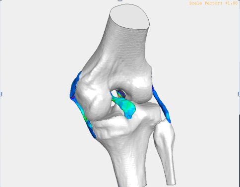
Figure: Maximum principal stresses in the ligaments of the knee. Courtesy M.H. Doweidar, University of Zaragoza (as presented in Doblaré & Merodio).

Such studies motivate student projects on ACL / PCL / MCL / LCL load sharing, graft prestress, and post-injury or post-reconstruction stress patterns in COMSOL.

COMSOL Multiphysics Implementation Outline

• Geometry: Idealised ligament bundles or patient-specific segmentation from MRI/CT; attachment sites on bone surfaces
• Materials: Nearly incompressible hyperelastic models (Neo-Hookean / Mooney–Rivlin matrix + fibre reinforcement via Holzapfel–Gasser–Ogden or transversely isotropic invariants); optional QLV or Prony series for time dependence
• Physics: Solid Mechanics (large deformation, geometric nonlinearity); contact at joints if multi-body knee model
• Loads / BCs: Displacement- or force-driven flexion–extension; residual stress via prestretch / multiplicative split or inverse design
• Outputs: Maximum principal stress maps, fibre stretch, reaction forces at insertions, comparison with toe/linear/failure regions of the experimental curve
• Cross-check tools: Ansys Mechanical / LS-DYNA, SIMULIA Abaqus, SimScale for selected load cases

Project Deliverables (Bangalore Support)

• COMSOL model notes (geometry, mesh, material cards, study steps)
• Stress–strain curve interpretation and constitutive parameter discussion
• Knee ligament stress contour figures and load-sharing tables
• University-format report (VTU / Anna University / JNTU style)
• PPT (20–25 slides) and viva Q&A focused on soft tissue biomechanics and COMSOL setup

Core soft-tissue and ligament concepts summarised from: Manuel Doblaré & José Merodio, An Introduction to Biomechanics and Mechanobiology (tissue biomechanics and mechanobiology chapter).