Comsol Pacemaker Lead Field

Abstract

The electromagnetic part of pacemaker lead heating during magnetic resonance imaging (MRI) is a resonant phenomenon which is complicated by, among other factors, the wide range of length scales involved in the problem. In this work, the multi-scale part of the problem is taken into special consideration during the model- ing process. The model incorporates a radio frequency coil, a human body phantom, and a highly detailed model of a pacemaker system with a bipolar lead.

Several configurations of pacemaker systems exposed to MRI are modeled and the results clearly show the importance of detailed lead modeling. Furthermore, model- ing of resonant structures is investigated by a comparison between different modeling techniques.

2.1

Challenges . . . . . . . . . . . . . . . . . . . . . . . . . . . . . . . . . . . . . . . . . . . . . . . . . . .

2.1.1

Inter-examination variability . . . . . . . . . . . . . . . . . . . . . . . . . . . . .

2.1.2

Body tissue heterogeneity . . . . . . . . . . . . . . . . . . . . . . . . . . . . . . .

2.1.3

Multi-scale problem . . . . . . . . . . . . . . . . . . . . . . . . . . . . . . . . . . . .

2.2

Related work . . . . . . . . . . . . . . . . . . . . . . . . . . . . . . . . . . . . . . . . . . . . . . . .

2.3

Proposed model . . . . . . . . . . . . . . . . . . . . . . . . . . . . . . . . . . . . . . . . . . . . . .

2.3.1

RF birdcage coil . . . . . . . . . . . . . . . . . . . . . . . . . . . . . . . . . . . . . . .

2.3.2

RF shield . . . . . . . . . . . . . . . . . . . . . . . . . . . . . . . . . . . . . . . . . . . . .

2.3.3

Human body phantom . . . . . . . . . . . . . . . . . . . . . . . . . . . . . . . . . .

2.3.4

Implant . . . . . . . . . . . . . . . . . . . . . . . . . . . . . . . . . . . . . . . . . . . . . . .

2.3.5

Standard model setup. . . . . . . . . . . . . . . . . . . . . . . . . . . . . . . . . . .

2.4

Performance measures . . . . . . . . . . . . . . . . . . . . . . . . . . . . . . . . . . . . . . . . .

3.1

Modeling of resonant structures based on the thin-wire approximation 13

3.1.1

Single helix . . . . . . . . . . . . . . . . . . . . . . . . . . . . . . . . . . . . . . . . . . . .

3.1.2

Double helix . . . . . . . . . . . . . . . . . . . . . . . . . . . . . . . . . . . . . . . . . . .

3.2

Modeling of pacemaker systems in MRI. . . . . . . . . . . . . . . . . . . . . . . . . .

3.2.1

Impact of lead length . . . . . . . . . . . . . . . . . . . . . . . . . . . . . . . . . . .

3.2.2

Impact of number of filars . . . . . . . . . . . . . . . . . . . . . . . . . . . . . . .

3.2.3

Impact of detailed modeling . . . . . . . . . . . . . . . . . . . . . . . . . . . . .

Introduction

The three electromagnetic fields present in magnetic resonance imaging (MRI) all interact with passive and active medical implants. The static field can create forces and torques on the implant whereas the gradient fields, which are in the kHz-range, can cause vibrations, electrical interference and nerve stimulation. The radio fre- quency (RF) field can cause severe highly localized heating near sharp corners and edges of an implant. In particular, elongated conducting implants, like deep brain stimulation and pacemaker leads, can suffer from severe heating at their ends.

Currently, the number of MRI examinations per year is steadily increasing at the same time as medical implants are becoming an integral part of modern healthcare. Unfortunately, the interactions described above causes active implantable medical devices to be classified as a contraindication for MRI, i.e.

A Patient With Such

an implant is not allowed to undergo an MRI examination. Although there are two commercially available pacemaker systems which are conditionally safe in MRI [1, 2] and several MRI examinations have been performed on pacemaker patients with- out negative effects , the interactions between the electromagnetic fields and the pacemaker system during MRI is still an important topic to investigate. Especially as the available conditionally MR safe pacemaker systems are only approved for 1.5 T MRI scanners and have certain limitations (large parts of the torso can not be imaged with the system in reference and the lead diameter is increased with respect to non MR approved leads with the system in reference ).

The electromagnetic fields generated by the RF coil of the MRI system induce currents in the body tissue and in the conductors of the implanted pacemaker lead. The lead constitutes a resonant structure and charge can be accumulated at its ends.

Near the ends with accumulated charge, strong electric fields heat the conductive body tissue by Joule heating. In order to further understand the factors influencing the heating, and ultimately to find a pacemaker lead design which is inherently safe in MRI, we model the electro- magnetic part of the problem. First, we discuss the modeling challenges (section 2.1) and previous modeling efforts presented in the literature (section 2.2). Next, we present our modeling approach in section 2.3 and in section 2.4 the performance measures used in this study are described.

In the results section (section 3), we characterize the approximations in our modeling by investigating resonant structures in section 3.1. Finally, we devote section 3.2 to the investigation of pacemaker systems in MRI, a study based on the proposed model.

Challenges

Modeling of pacemaker lead heating during MRI faces three major challenges which are described below.

Inter-Examination Variability

Several factors with strong impact on the lead heating show large variations be- tween different patients and healthcare establishments. For example, the type of MRI machine and examination (RF field strength, imaging sequence, duration of the imaging procedure, body structure being imaged) vary between examinations.

Furthermore, the patient position in the RF coil, the position of the pacemaker and lead configuration inside the patient, and patient characteristics (size, morphology, posture) are different for different examinations. In addition, variations exist in length and design of the pacemaker lead as well as in the type of implanted device.

Thus, the number of different combinations of the factors mentioned above is vast wherefore individual simulations of each combination is an intractable approach.

Body Tissue Heterogeneity

The different tissue types present in the human body are both geometrically complex and differ strongly in dielectric properties. For example, Liu et al. used conductiv- ity values from 0.02 S/m (yellow marrow) to 2.3 S/m (cerebrospinal fluid) and values for the relative permittivity from 7 (fat and mammary tissue) to 128 (intestine/bowel content) in their simulations of an MRI system operating at 64 MHz. Volume dis- cretizing computational methods, such as the finite element method (FEM) and the finite-difference time-domain method (FDTD), are normally preferred to boundary discretizing methods, such as the method of moments (MoM). This is due to the higher computational cost of MoM, when compared to the FEM and FDTD, for simulations that exploit highly detailed human body models.

Multi-Scale Problem

Several length scales are present in the problem. At 64 MHz, the wavelength λ0 of the RF field in free space is roughly five meters. Thus, the human body has a size of approximately λ0/3. Inside the body, the wavelength is reduced to λ = λ0/√εr

Modeling

where εr is the relative permittivity of the body tissue. Despite this reduction of the wavelength, some components of the pacemaker lead have dimensions on a length scale of approximately λ/1000.

Volume Discretizing Methods Are Able To Resolve

these length scales concurrently but suffer from overwhelming simulation times and memory requirements.

Related Work

Previously, Yeung et al. used the MoM to model bare and insulated, straight wires in an infinite homogeneous lossy medium. They used this model to investigate the impact of the wire diameter, the insulation permittivity and thickness, and the tissue conductivity. The same authors also used this model in reference to study the impact of the phase distribution of the external field. By changing this phase they constructed an excitation with maximal heating. The same type of modeling and ideas was elaborated on by Park et al. [7, 8] who developed a transfer function that relates the tangential part of the external field impingent on a small part of the lead with the electric field near the end of the lead. Different, more complex, lead designs were compared by Bottomley et al. without resolving their finer details.

Modeling with detailed anatomical models based on the FDTD technique was per- formed by Pisa et al. and Mattei et al. where the latter valdiated the RF coil model against experiments. Furthermore, Vogel et al. showed that the FEM can be used for lead heating simulations by modeling an entire examination room with an open MRI system. However, all these studies used simple lead models.

A more ambitious study was performed by Park et al. who used 100 lead paths in each of 22 different human body models to compute the dissipated power at the lead tip using FDTD. Animal tests (dogs) were then performed where a lead was end-fed with RF-power of different levels and the corresponding change in pacing capture threshold (a significant marker for tissue heating) was measured. By com- bining the two populations of results, a probability curve could be generated which gave the probability for the entire range of changes in pacing capture threshold.

Unfortunately, it is unclear how the leads were modeled. The most detailed lead modeling available in the literature is presented by Neufeld et al. . They used a two-step method with FDTD to fully resolve a single helix- shaped conductor. The results were then compared to measurements on the same lead and the difference between these results was shown to be within the uncertainty range through a sensitivity analysis.

However, modern pacing leads have geometries that are more complex than the one examined by Neufeld et al. In addition, experiments performed by Bottomley et al. show that the finer details of the pacemaker lead strongly influence the heat- ing around the lead tip. Therefore, we continue and extend our work presented in reference and focus on pacemaker systems with a wide range of length scales

5

modeled simultaneously. In particular, we use the MoM which discretizes bound- aries between dielectrically different media. In order to keep the problem size within feasible limits, we simplify the complexity of the human body by modeling it as homogeneous according to the test standard ASTM F2182-09 . Apart from the multi-scale modeling, this simplification has the additional advantage that it enables comparison of the results with results from controlled measurements. Such compar- isons could prove difficult if highly detailed models, such as the Virtual Family , were used.

Proposed Model

We aim at modeling the RF part of the ASTM test standard which describes a lead heating experiment for cylindrical bore MRI systems. Here we consider such a system with a 1.5 T static magnetic field. The model contains an RF birdcage coil, an RF shield, a human body phantom, and an implanted pacemaker system consisting of a pacemaker unit and a bipolar lead. Each part of the model is explained in detail below. Our modeling environment is modularized to provide flexibility and it uses the frequency domain MoM available in the commercial software Efield R⃝[18, 19].

Rf Birdcage Coil

We model a generic RF birdcage coil consisting of two end rings connected by a variable number of equally distanced rungs. An example of a coil mesh is shown in figure 2.1. Both the end rings and the rungs are modeled by infinitely thin strips which are discretized with triangles. The entire coil is modeled with a perfect electric conductor (PEC) material. The coil is monochromatically excited at 64 MHz by a voltage source at the middle of each rung. All sources are assigned unit amplitude with a linear phase variation of 2π around the circumference of the coil. This models the currents that yield an RF field that is homogeneous in the center region of the coil, which is desired for MRI. Normally, real-life coils are fed only at two points on one of the end rings and the desired RF field with rotating magnetic field vector is obtained at the desired frequency by tuning capacitors. The feeding used in our model yields similar currents as with the real-life feeding but without having to tune any capacitors. Further information on different approaches for modeling birdcage coils can be found in reference , where the FDTD method was used.

Rf Shield

RF shields are used to shield the space outside the coil from the RF field and also to shield the RF coil from interactions with the surroundings since such interactions can have negative impact on the performance of the RF coil. We model the RF

Y

Figure 2.1. A 16-rung RF birdcage coil surrounded by an RF-shield. The source positions on the coil rungs are marked with black dots.

shield as a cylindrical shell sharing symmetry axis with the birdcage coil. The RF shield is assigned a PEC material in the model. An example of an RF shield mesh is shown in figure 2.1.

If the RF shield is placed close to the coil and extends beyond the ends of the coil, the image of the birdcage coil in the RF shield is in itself a birdcage coil with currents flowing in the opposite direction as compared to the currents on the original coil . The field pattern inside the coil is therefore not significantly influenced by the presence of an RF shield. However, the field strength inside the coil is reduced due to the image currents. Depending on the purpose of the modeling and the type of model used for the birdcage coil, the RF shield can in many cases be excluded from the model without any major impact on the quantities of interest.

7

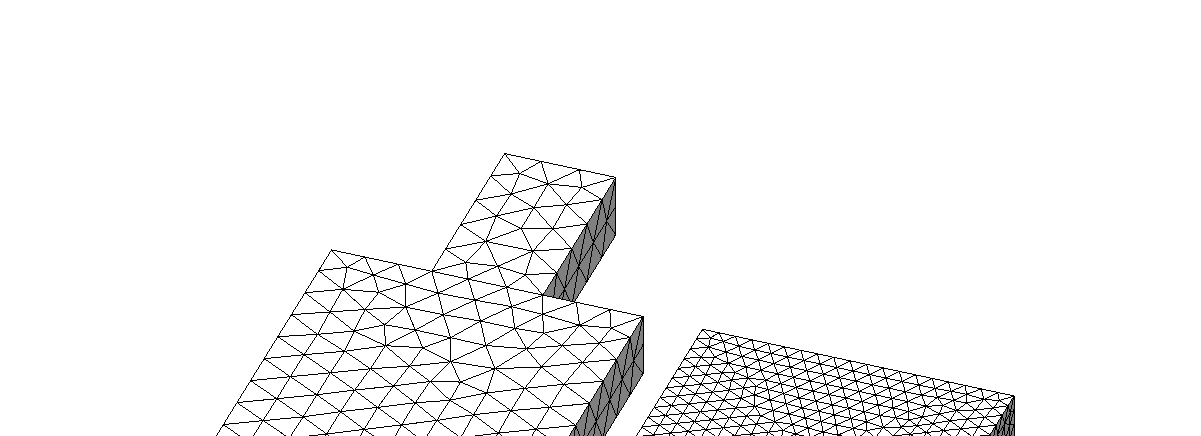
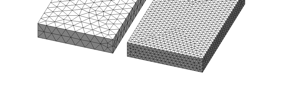
Figure 2.2. Surface meshes of two human body phantoms: with head and maximum element size of λ/10 (left), and without head and maximum element size of λ/20 (right).

Human Body Phantom

We use a homogeneous body phantom according to the ASTM test standard . The phantom is shaped as a rectangular block filled with a lossy dielectric and it is intended to mimic the torso of an adult. The presence of a head on the phantom is optional. We use COMSOL Multiphysics to create two models of the phantom, one with and one without the head. COMSOL is also used to mesh the phantoms’ surfaces and to export the meshes to our simulation environment. Examples of these meshes are shown in figure 2.2.

Implant

We model a pacemaker system consisting of a pacemaker unit and a bipolar lead. The lead has two helix-shaped coaxial conductors: one inner conductor and one outer conductor which are modeled with straight segments using the MoM thin- wire approximation. In turn, each conductor consists of one or several filars, which are connected at each end of the lead but otherwise insulated from each other.

Modeling

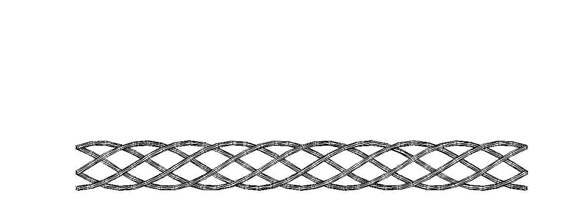
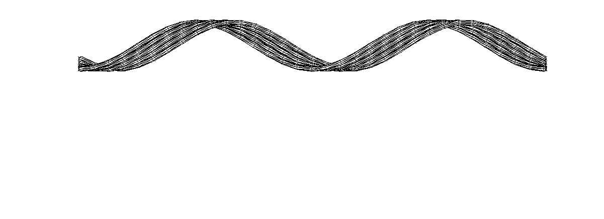
Figure 2.3. Equidistant (top) and tight (bottom) filar winding. (Should the filars not be insulated from each other, a modeling approach based on a conducting strip instead of a set of wires could prove useful.) In figure 2.3, two different filar windings are shown. In the upper part of the figure, the filars are equidistantly spread along the turn whereas they are tightly packed in the lower part of the figure, i.e. wound in such a way that the filars are almost touching. The conductors/filars are meshed using the area compensating scheme described in which reduces the number of wire segments needed per turn for a certain discretization error. The conductors are fully enclosed in a tube of insulating dielectric.

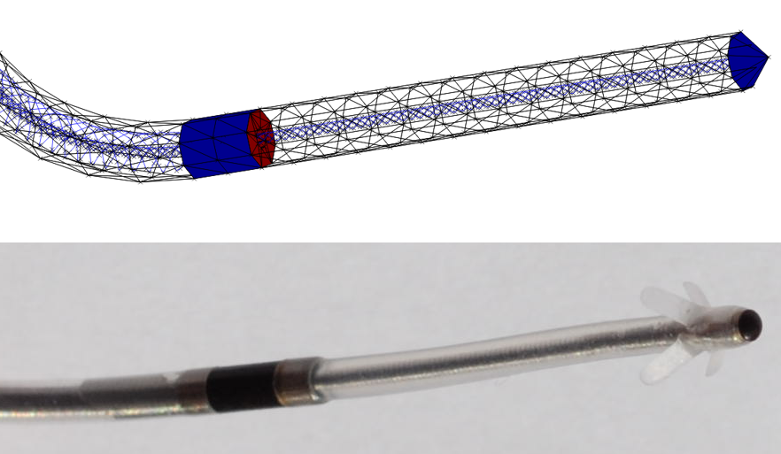
The distal end of the lead, i.e the end of the lead which connects to the heart, features a tip electrode and a ring electrode that are modeled as PEC. This models a pacemaker lead with passive fixation where the tines have been left out. The inner conductor connects to the backside of the tip electrode whereas the outer conductor connects to the backside of the ring electrode. The boundary conditions assigned to the electrode surfaces impose a purely tangential current which means that current can not enter nor exit the lead at these electrodes. This model is a simplification of the corresponding physical situation that is far more complex, see for example reference for more details on the contact impedance and related matters. Figure 2.4 shows a mesh of the distal end of the lead together with a photo of a clinical pacemaker lead.

The path followed by the lead in space, or the lead configuration, is described by a parametric curve Γ : (x(s), y(s), z(s)) , s ∈[0, 1].

The Surface Elements Of The

insulation and the two electrodes are generated as follows. At the start (s = 0), a local coordinate system (⃗u,⃗v,⃗w) is chosen such that⃗w is parallel to the tangent of the lead path. A number of points are placed evenly on a circle in the uv-plane before a step is taken along Γ by letting s = δs. Once again the tangent vector along Γ is set as⃗ws=δs. The basis vector⃗us=δs is now obtained as the part of⃗us=0 which is orthogonal to⃗ws=δs. The same number of points as before are now placed evenly on a circle in the uv-plane. Triangular elements are created using these two rings of points. The procedure continues similarly until the end of the lead s = 1. Thus, a tubular shell is obtained. The shell can be closed at the ends by inserting a point at

9

Figure 2.4. Photo of a clinical pacemaker lead (top) and a mesh of the same part of the lead (bottom).

the origin of the first/last local coordinate system and adding triangles between this midpoint and the points on the boundary of the tubular shell. The midpoint can also be displaced a small distance in the (−w/ + w)-direction to generate a pointed tube. Note that it is important to reuse⃗us=s1 when generating⃗us=s1+δs in order to save the tube from twisting, which could render the mesh useless.

The wire segments of the conductors are created using the same approach as above with local coordinates. The difference is that at each s only one point is added on the circle in the uv-plane. The angle between the point and⃗u is a linear function of s which generates a helix when the points corresponding to two neighboring values of s are connected with a line segment.

A pacemaker unit is placed at the other end of the lead compared to the electrodes. The pacemaker unit is modeled as a hollow rectangular box made of PEC mate- rial filled with insulation. The pacemaker measures 6 cm × 6 cm × 1 cm and it is meshed using COMSOL with a maximum element size of λ/50. The conductors enters through a circular hole in the pacemaker. Inside the pacemaker, the inner conductor is connected to the outer one through a lumped component which models the electronics of the pacemaker unit. The outer conductor is also connected to the metal shell of the pacemaker unit through a lumped component. A mesh of a pacemaker lead with an attached pacemaker unit is shown in figure 2.5.

Simulations without the pacemaker unit can also be performed. In this case, the lead ends with the two conductors being connected through a lumped component, where the termination of the two conductors and the lumped component are embedded in

Modeling

Figure 2.5. Mesh of a pacemaker lead with an attached pacemaker unit. the insulation of the lead.

Standard Model Setup

The parameter values stated below are used throughout this work unless stated otherwise.

Rf Birdcage Coil

The standard model setup uses a birdcage coil modeled with patches and parameters according to table 2.1. The birdcage coil operates at 64 MHz and is excited as described in section 2.3.1.

0.01 M

Table 2.1. Parameter values for the standard setup of the birdcage coil.

Rf Shield

Since our model of the birdcage coil does not include tuning capaci- tors and the fields are scaled to obtain a specified specific absorption rate (SAR) level in the phantom, the RF shield has no impact on the simulation results (see section 2.3.2). It is therefore excluded from the standard setup.

The Standard Model Setup Uses The Head-Less Human

body phantom described in the test standard with parameters according to table 2.2.

Implant

The standard model setup uses an insulated bipolar pacemaker lead in- serted into the human body phantom. The electrical conductors of the lead are mod- eled using the thin-wire approximation. The corresponding parameters are listed in table 2.3.

Λ/20

Table 2.2. Parameter values for the standard setup of the human body phantom.

Performance Measures

The test standard ASTM F2182-09 uses two performance measures: the local SAR and the local additional temperature rise with the implant in place. The SAR

(2.1)

where σ is the electric conductivity of the tissue, E is the electric field phasor, ρ is the density of the tissue,⃗r is the position vector, and Ωthe region of tissue over which the quantities are averaged. These two performance measures are also common in previous modeling, for example Neufeld et al. and Yeung et al. .

In order to model the temperature rise, a heat problem must be solved where the result of the electromagnetic simulation is used as source term. However, we are, at least in a first step, interested in relative instead of absolute performance measures since our aim is to compare the heating performance of different lead designs. In addition, the heat equation has a smoothing effect on the distribution of the source term, see for example , wherefore we use different electromagnetic quantities as performance measures instead.

At least three different performance measures can be used:

• Electric Field Around Implant Electrodes

The tissue is heated by Joule heating.

These Power Losses, And The Corre-

sponding source term in the heat equation, are proportional to the square of the absolute value of the electric field. This measure is very closely related to the SAR, as defined in equation (2.1), with the advantage of not having to decide over which mass of tissue the quantity should be averaged.

• Accumulated Charge On The Electrode Surfaces

The electric field in the electrode vicinity is proportional to the accumulation of charge on the electrode surfaces.

• Maximum Value Of The Induced Current

The accumulation of charge at the ends of the lead is associated with currents

N/A

Helix length (excluding the part from tip to ring)

No

Table 2.3. Parameter values for the standard setup of the implant.

If Two

values are listed they should be read as (value for inner conductor, value for outer conductor). induced in the lead by the tangential component of the external field. An increase in tissue heating is due to stronger electric fields and currents in the tissue. The increase of these fields and currents is associated with increases in accumulated charge and induced currents on the lead.

Thin-Wire Approximation

The conducting wires in pacemaker leads are normally shaped as helices. The helix length is comparable to the wavelength of the RF field in the human body but the helix diameter is far smaller than the wavelength. Below, we therefore investigate the electromagnetic properties of helices and especially the impact of the helix pitch angle. We also study the validity of the thin-wire approximation when applied to modeling of helices.

Comparison With Surface Discretization

In order to investigate the validity of the thin-wire approximation when modeling resonant structures, such as a pacemaker lead, we model a single helix in free space excited by a plane wave. The plane wave is polarized along the helix axis and it im- pinges on the helix perpendicularly to this axis. A frequency interval corresponding to Lwire/λ ∈[0.1, 6.1] is studied where Lwire is the total wire length.

The helix has the following characteristics: 90 turns, wire diameter d, outside helix diameter 11d and pitch height 1.1d which corresponds to a pitch angle Ψ = 2.0◦and an inter-turn distance of 0.1d. That is, the turns are almost in contact with each other. The wire and helix diameters are both significantly shorter (< 2.4%) than the wavelength of the plane wave at the highest frequency.

The problem is solved using the thin-wire approximation as well as using a stan- dard MoM approach where the surface of the wire is discretized. To assure a fair comparison between the results, one thin-wire segment models the same part of the helix wire as a straight cylinder does in the surface discretization. The surface discretization is expected to give a more accurate result since it permits current distributions that are not constant around the circumference of the wire as assumed by the thin-wire approximation. In addition, it can model currents flowing in the circumferential direction of the wire. A part of the geometry is shown in figure 3.1 for the two different representations.

The maximum absolute value of the induced current is shown in figure 3.2 as a function of the total wire length normalized by the wavelength over a frequency band. Clearly, the resonant frequencies obtained with the thin-wire approximation

Results

Figure 3.1. Thin-wire representation (left) and surface representation (right) of a couple of turns of the single helix.

are shifted to higher frequencies compared to their counterparts from the surface dis- cretization. However, the overall current amplitude is very similar between the two modeling techniques. Similar simulations suggest that the difference in resonance frequencies decreases when the pitch angle increases. For example, the relative error in amplitude is smaller than 6% at the first resonance for Ψ = 17◦.

Impact Of Helix Pitch Angle

A helix is defined by four geometrical parameters: the helix length, the pitch angle Ψ, the wire diameter, and the helix diameter. The helix length can also be described by the number of helix turns or the total wire length Lwire. Likewise, the pitch angle can be replaced by the pitch height in the description of the helix.

We investigate the impact of the pitch angle on the resonant frequencies of the helix by exploiting the same model as above at Ψ = 2◦. The pitch angle is then increased

In Two Different Ways:

1. Lwire is kept constant. As a consequence, the number of helix turns and the helix length change when the pitch angle is varied. 3.1 Modeling of resonant structures based on the thin-wire approximation

Thin−Wire Current

Figure 3.2. Maximum amplitude of the induced current obtained with thin-wire and surface modeling vs. normalized wire length at a helix pitch angle of Ψ = 2◦.

Note that the wire length has been scaled with respect to the wavelength, λ, of the incoming plane wave. 2. The number of turns is kept constant and, therefore, Lwire and the helix length change when the pitch angle is varied.

The wire and helix diameters are constant (and identical) in both cases. The helix is modeled using the thin-wire approximation. Figure 3.3 shows the maximum amplitude of the induced current on the helix as a function of the pitch angle and the frequency of the incoming field for the case where Lwire is kept constant. Note that the frequency is expressed as the total wire length divided by the wavelength λ and that the current scale is logarithmic. In the limit Ψ →90◦, the obtained results agree well with the standard results for dipole

Antennas Where Resonances Occur At Lwire = (N + 1

2)λ, n = 0, 1, 2, . . .. When the pitch angle decreases, the resonances shift to higher frequencies. Fur- thermore, they also get more distantly spaced in frequency until the pitch angle reaches 10◦. Below this angle, the resonances quickly move to lower frequencies and approach each other.

−2

Figure 3.3. Maximum amplitude of the induced current vs. normalized wire length and helix pitch angle Ψ. The wire length is constant for all pitch angles but the number of turns and helix length changes. Note that the wire length has been scaled with respect to the wavelength, λ, of the incoming plane wave and that the current scale is logarithmic.

The corresponding results for the case where the number of turns is kept constant are shown in figure 3.4. The overall behavior is similar to the first case. However, it can be noted that the induced currents are stronger in the limit Ψ →90◦for this second case. Furthermore, the decrease in resonant frequencies for Ψ < 10◦can be more clearly seen for the second case than for the first case.

3.1 Modeling of resonant structures based on the thin-wire approximation

−2

Figure 3.4. Maximum amplitude of the induced current vs. normalized wire length and helix pitch angle Ψ. The number of turns is constant for all pitch angles but helix and wire lengths change. Note that the wire length has been scaled with respect to the wavelength, λ, of the incoming plane wave and that the current scale is logarithmic.

Related Journal Articles & DOI Links

Selected peer-reviewed publications relevant to 12 Lead ECG Acquisition. Click the DOI to access the full paper (may require institutional access).

Why Choose Us?

Bangalore guidance for robotics, Spectre and autonomous systems projects.