Comsol Photoacoustic Imaging

Developed

dramatically and witnessed a lot of applications in various fields over the past few years. This boom originated in 2009, when a new model emerged, that is, the deep artificial neural network, which began to surpass other established mature models on some important benchmarks. Later, it was widely used in academia and industry. Ranging from image analysis to natural language processing, it fully exerted its magic and now become the state-of-the-art machine learning models. Deep neural networks have great potential in medical imaging technology, medical data analysis, medical diagnosis and other healthcare issues, and is promoted in both pre-clinical and even clinical stages. In this review, we performed an overview of some new developments and challenges in the application of machine learning to medical image analysis, with a special focus on deep learning in photoacoustic imaging.

The aim of this review is threefold: (i) introducing deep learning with some important basics, (ii) reviewing recent works that apply deep learning in the entire ecological chain of photoacoustic imaging, from image reconstruction to disease diagnosis, (iii) providing some open source materials and other resources for researchers interested in applying deep learning to photoacoustic imaging.

I. Introduction

The advent of the era of big data, the increase in computing power following Moore's Law, and open-source, user-friendly software frameworks have made remarkable progress in machine learning, which has aroused great interest in both industry and academia. Data-driven artificial neural networks, also known as deep learning (DL) [5, 6], are good at discovering complex patterns from massive data to determine the optimal solution in the parameter space. The growing computing power of GPUs allows neural networks to be flexibly expanded from depth [7, 8], width , and cardinality , forming numerous cornerstone-like models, which have also become the state-of-the-art (SOTA) approaches for a series of problems, exerting its magical power in computer vision, natural language processing and robotics.

Among The Many Image Analysis Benchmarks, Deep

learning rapidly surpasses the traditional machine learning +Those authors contributed equally to this work. Changchun Yang, Hengrong Lan, Feng Gao and Fei Gao are with the Hybrid Imaging System Laboratory, Shanghai Engineering Research Center of Intelligent Vision and Imaging, School of Information Science and

China

Changchun Yang and Hengrong Lan are also with the Chinese Academy of Sciences, Shanghai Institute of Microsystem and Information Technology, Beijing 100049, China.

technology, making it reach the most important position in computer vision. At the 2012 ImageNet Large-Scale Visual

Recognition Challenge (Ilsvrc, ), A Convolutional

neural network, AlexNet, easily exceeded the support vector machine (SVM) to win the championship with a disparity of more than 10%. That is, since this session, deep learning has replaced SVM, and various innovative neural network models have sprung up. The Top-5 error rate used to measure performance has also reached new lows under fierce competition, gradually surpassing human eye recognition (5~10%), and even close to the Bayes error rate. In addition to shining in computer vision, deep learning also shows its advantages in areas such as natural language processing [12, 13], speech recognition [14, 15]1, and even the field of physics 2.

By hybrid combination of high contrast of optical imaging

And High Penetration Depth Of Ultrasound Imaging,

photoacoustic (PA) imaging, one of the non-invasive medical imaging methods [19, 20], has undoubtedly become an emerging application of deep learning. Therefore, we will review recent research of PA imaging (PAI) with deep learning.

A. Pa Fundamental Physics

Many literatures have introduced the fundamentals of PAI

, Here We Only Give A Brief Review Of Pai In This

section. In PAI, several transducers are used to detect the broadband PA signals, which are excited by a nanosecond pulsed laser light. The initial PA pressure can be expressed as:

(1)

where Γ0 is the Gruneisen parameter of tissue, ηth is the energy conversion efficiency from light to heat, µα is the optical absorption coefficient, and F is the local optical fluence.

After the generation of p0, the PA wave propagation in the medium can be described by the following PA equation: 1 DeepMind proposed a deep generative model of raw audio waveforms,

Voice:

https://deepmind.com/blog/article/wavenet-generative-model-raw-audio. 2 Modern deep learning methods have also achieved some applications in the field of physics, and these methods are often highly transferable across domains, such as cleaning of interference images in astrophysics and denoising in gravity wave analysis , which use a combination of mathematical models and machine learning models to learn the relationship of physics from raw data. These methods can also be used in medical image analysis [18, 19].

Review Of Deep Learning For Photoacoustic Imaging

Changchun Yang+, Hengrong Lan+, Feng Gao, and Fei Gao*

(2)

where p(r,t) is the PA pressure at position r and time t, T is the temperature rise, κ is the isothermal compressibility, β denotes the thermal coefficient of volume expansion, and vs is the speed of sound. In PAI, the short laser pulse duration should satisfy two confinements: the thermal diffusion time (τth) and the stress relaxation time (τs). Namely, the laser pulse duration should be much less than τs and τth. The thermal

(3)

if the laser pulse duration satisfies above condition. The H denotes the heating function, which is defined by the product of the optical absorption coefficient and fluence rate (H=µαΦ).

Substituting Eq. (3) into Eq. (2), we obtain the following

(4)

where CP denotes the specific heat capacity at constant pressure. We can solve this equation with Green function :

(5)

where p0(r’) is the initial pressure at position r’.

B. Pai Modalities

Two fast growing modalities of PAI are photoacoustic microscopy (PAM) and photoacoustic computed tomography (PACT). They obtain images in different ways: the former is point-by-point scanning formed image, and the latter is reconstructed image by acquiring PA signals at different positions.

For PAM, a focused ultrasound transducer is used to scan along the tissue surface. In general PAM setup, both the optical illumination and acoustic detection are confocal. Two typical PAMs are optical-resolution PAM (OR-PAM) and acoustic-resolution PAM (AR-PAM), which depend on either the optical focus or the acoustic focus is finer. OR-PAM can provide a high lateral resolution from a few hundred nanometers to a few micrometers with a high frequency transducer. The PA signal’s penetration is limited since the high frequency PA signal suffers severe acoustic attenuation.

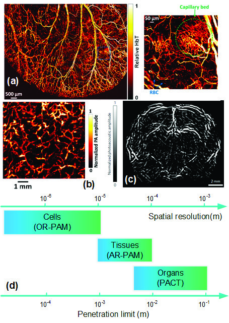
OR-PAM can provide the vascular anatomy and label-free imaging for hemoglobin oxygen saturation (sO2) as shown in Fig. 1(a) . On the other hand, AR-PAM has a tighter acoustic focus than the optical focus. It achieves resolution of tens of micrometers with acoustic diffraction-limited. The imaging speed of AR-PAM is limited by the scanning speed and the pulse repetition rate of the laser. In Fig. 1(b), AR-PAM can achieve a larger-scale vasculature imaging .

Moreover, low scanning speed and small scanning range also limit the applications of PAM. To accelerate the speed of imaging, PACT uses ultrasonic transducer array to receive PA signals at different positions.

An expanded laser beam evenly excites the entire region of interest (ROI), and the PA waves are detected by transducer array simultaneously. After that, reconstruction algorithms, such as universal back-projection (UBP) and time-reversal (TR) [28, 29], are used to reconstruct a high resolution image.

PACT with spatial resolution of hundreds of micrometers is preferred, which can be improved by increasing the central frequency and bandwidth of the transducer array. PACT can achieve the whole-body small animals and some organs of human, such as shown in Fig. 1(c) [30, 31].

Generally speaking, the achievable spatial resolution can be estimated if the imaging depth is determined. We list the different spatial resolutions and penetration limits for different PAI modalities in Fig. 1(d).

Iii. Deep Learning

It is the core of machine learning to develop some algorithms to make computers capable of learning experience from data to solve tasks. A mathematical model f is created to produce the desired output through training when fed with Fig. 1. (a) Representative image of OR-PAM imaging a mouse ear, RBC: red blood cell, reproduced with permission from .

(b) Representative image of AR-PAM imaging a palm of a volunteer, figures adapted with permission from . (c) Representative image of PACT imaging a mouse head, figures adapted with permission from . (d) The different spatial resolutions and penetration limits for different PAI modalities, figures adapted with permission from .

input data. The training set contains rich data representation information, which can provide experiences for machine learning models. Those models that learned the representation of data are then tuned to produce accurate predictions according to the difference between current predicted output and the expected output by an optimization algorithm. The feedback obtained by training the model on another separate data set, the validation set, is used for further fine-tuning to measure the generalization ability of the model. After iterating through these two steps (tuning and fine-tuning), the model is finally evaluated on the test set to evaluate the performance when it encounters new, unseen data. Tuning, fine-tuning, and evaluation are also the necessary three steps of machine learning to evaluate whether your mathematical model f can solve your task perfectly.

We roughly divide machine learning into three categories here according to the training process. First category is the

The

constructed agent and the environment achieves the greatest benefit or solves specific problems through learning strategies. One of its most famous applications is AlphaGo , which is a Go-playing system developed by DeepMind, even defeating the world’s top Go players. The second category is unsupervised learning that is to classify or group

Based On Training Samples With Unknown Categories

(unlabeled) and discover patterns between them. A common unsupervised learning example is cluster analysis. The last category is supervised learning, paired data sets make mainstream machine learning algorithms focus on it. Train on the labeled data to find the rules of patterns, and then produce the correct label on the unseen data. For example, many

Medical Imaging Including Pa Image Reconstruction

problems [33, 34] are based on supervised learning. Regarding machine learning, especially deep learning, many excellent reviews and surveys have also emerged, you can check the relevant papers for a short introduction, or read free available book 3 for an in-depth understanding.

See also for a broad understanding of its application to medical image analysis. Only some basic essentials of deep learning will be introduced in this section, serving as useful foundations for its application in PA imaging.

A. Artificial Neural Networks

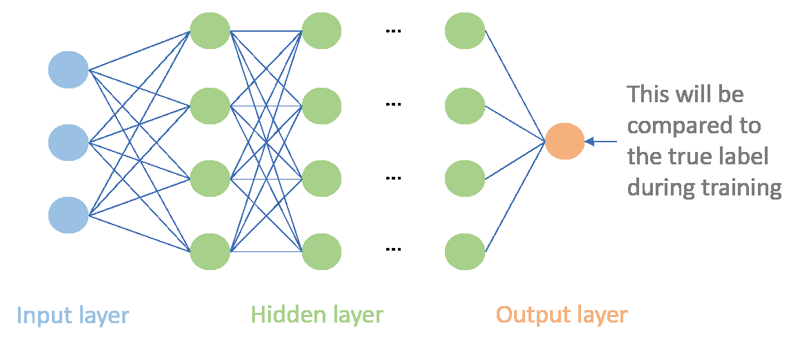
Firstly we will introduce one of the most famous machine learning models that appeared in the 1950s, the artificial neural network, which is used to briefly explain the deep learning principle. A neural network is composed of many layers, which are connected by many computing units, also known as neurons. Data enters the neural network through the input layer, then flows through one or more hidden layers, and finally generates the prediction of the neural network in the output layer, which will be compared with the actual labels (ground truth) by an objective function (loss/cost function).

This difference guides to change the weights of the network to optimize the objective function until the neural network produces a good prediction. This means that the neural network learns experiences from the data and can generalize to new data sets for prediction.

Next, we will briefly explain how the artificial neural networks are constructed. Since the neural network can be very complex and deep, we only introduce its basic form4



.

,

followed by a simple linear transformation and a nonlinear function.

Is The Model’S Weights, And The Nonlinear

functions are differentiable, typically are sigmoid function and ReLUs. The basic idea of training a neural network is simple: training data flows into the network in the forward process, and the gradient of the loss function with respect to every weight is computed using the chain rule, finally gradient descent (GD) is used to change these weights to make the loss smaller . The reason why such a simple but effective idea did not start explosive growth until recent decade is

Version:

https://www.deeplearningbook.org/. 4 These are basic but essential concepts and components, compared to recurrent neural networks (RNNs), generate adversarial networks (GANs), graph convolutional networks (GCNs), etc.

Fig. 2. We take the most common artificial neural network, multilayer perceptron or feedforward neural network as an example. The output of the j-th unit at layer i-th is

,

where x is the value of the output of the previous layer after the nonlinear function transformation called activation function. Similarly, the output of each layer is passed to the next layer after the activation function, and then the same calculation is performed until the network produces the final output. The training data is fed to the input layer and then the streaming calculation is performed, where the output and derivative of each node are recorded. Finally, the difference between the prediction and the label at the output layer is measured by the loss function.

The choice of loss function has a critical impact on the performance of the entire task, so its choice is crucial, common ones include mean absolute error, mean squared error. You can also manually design the loss function, which is often more attractive. The derivative of the loss function will be used as a feedback signal, and then propagate backward through the network, and the weight of the network will be updated to reduce errors. This is a technique called backward propagation [36, 37], which follows the chain rule to calculate the gradient of the objective function with respect to the weights in each node. Then gradient descent is used to update all the weights.

because that when faced with the exponential growth of parameters and nodes, the calculation will be a huge challenge. Therefore, many techniques5 such as the design and training of neural networks are open and interesting problems.

B. Deep Learning

Traditional machine learning models will extract features from the data manually or with the help of other simple machine learning models before training. However, deep learning will automatically learn representations and features from the data during the training process, without the need for manual design. The main common feature of various deep learning models and their variants is that they all focus on feature learning: automatic learning of data representation, which is also the main difference between modern deep learning and classic machine learning methods. Learning features and performing tasks are improved simultaneously in the model. You can get a comprehensive understanding through the reference [5, 6], or have a detailed study of deep learning with an interactive book 6 whose codes use the most popular deep learning framework pytorch 7 in academia today.

Deep learning has made rapid progress in medical imaging, mainly relying on convolutional neural networks 8 (CNNs). This benefits from the fact that CNNs can easily learn specific features from images or other structured data. Next, we will briefly introduce the essential components of CNNs, 5 Applying deep learning in photoacoustic imaging, recently reported network architecture is significantly more complicated, such as that with multiple outputs , the input connected with the output , multiple branches , multiple loss functions , and much more. How to design a novel architecture that can solve specific task is the core.

6 Free available link: https://d2l.ai/. 7 Deep learning frameworks undoubtedly facilitate the process of machine learning practitioners turning ideas into code. The well-known ones are: tensorflow , pytorch , MXNet , and caffe . The first two are currently the most commonly used frameworks in industry and academia.

8 CNN has been used for medical image analysis in the early 1990s, but it was limited by the data and computing power at that time. understand why it is powerful and have an insight to design your own architecture.

C. Building Cnns

Although the introduced artificial neural network can be directly applied to the image, the efficiency of connecting each node of all layers to all nodes of the next layer is very low.

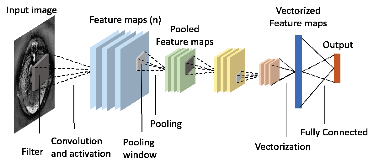
Fortunately, structured data such as images can be trimmed and connected based on domain knowledge. CNNs are neural networks that can preserve the spatial relationship between data with few connections. The training process of a CNN is exactly the same as ANNs, except that the structure is often convolutional layers accompanied by activation functions, and pooling layers (as shown in Fig. 3).

(i) Convolutional layers. In the convolutional layer, the activations from the previous layer performs a convolution operation with a parameterized filter 9. Each filter shares weights over the entire scope, which not only can greatly reduce the number of network parameters, but also has the translational equivariance. The reason why weight sharing can work is because features that appear in one part of the image may also appear in other parts. For example, this parameterized filter can detect the horizontal line above the image after training to determine the weight, then it can still detect the horizontal line below. After the convolution operation of the convolution layers, a tensor of feature maps will be generated.

(ii) Activation layers. Similar to the introduction in ANNs, the activation layer is often composed of nonlinear activation functions. Typical activation functions are sigmoid function

. There Are Also Many Other Types Of

activation functions, which can be selected depending on the task and architecture. Because of the existence of these 9 It can be compared to the filter in digital image processing, the “convolution” operation here is strictly the correlation operation, but called the “convolution” neural network is also appropriate.

Fig. 3. Construction of a typical CNN for medical image analysis, modified according to , and input image was taken from . nonlinear activation functions, combined with linear operations such as convolution, the neural network can almost approximate any nonlinear function [40, 41]10. See [42, 43] to learn more about the role of activation function. The activation layers also generate new tensors of feature maps.

(iii) Pooling. In neural networks, feature maps are often pooled in the pooling layer. The pooling operation generates a number for each small grid of the input feature maps, which is often achieved by max-pooling or average pooling. The significance of the pooling layer is to give the neural network translational invariance, since a small shift in input will result in changes in the activation maps. For example, to determine whether there is red in the image, translation/rotation will not affect the judgment result. Recent research also proves another alternative to pooling: using convolutional layers with larger stride lengths instead, which can simplify the network structure without reducing performance. Fully convolutional networks (FCNs) are also favored by more and more image analysis tasks.

(iv) Dropout. A very simple idea has greatly improved the performance of CNNs. Dropout is an averaging technique based on stochastic sampling of neurons to prevent CNNs from overfitting. By randomly removing neurons during the training process, each batch of data uses a slightly changing network, and the weights of the network will be tuned based on the optimization of multiple variations of the network.

(v) Batch normalization. Batch normalization (BN) 11 is an effective technique to accelerate deep networks training by reducing internal covariate shift. Due to changes in network parameters during training, the distribution of network layer output results is different, making network training difficult.

BN can produce normalized feature maps by subtracting the mean and dividing by the standard deviation for each training batch. The data will be periodically changed to zero mean and unit standard deviation with BN, which will greatly speed up the training.

10 No matter how deep the linear operation is, it can still only approximate the linear function without these nonlinear activation functions. 11 There is no unified conclusion about whether the position of BN is placed after convolution before activation, or after activation. The original paper put it before activation.

In The Actual Design And Improvement Of The Cnn

architecture, above basic components will be combined in a very complex way, with some new and effective operations. When building a CNN for a task, you often have to consider a lot of details to get your CNN perform well on this task. You need to fully understand the task to be solved and find insights to decide how to process the data set before fed to the network.

In the early days of deep learning, the construction of modules was often simple. But then more and more complicated structures emerged, and people designed new effective architectures based on previous ideas and insights resulting in updates to the SOTA. See for a survey about recent architectures of CNNs. These novel architectures are often suitable for PA imaging. The structure of most articles we researched can be inspired by them. But before the data is fed into the network, the signal domain12 or image domain13 will be processed separately to reduce noise or increase contrast.

Table 1. Number of papers of DL in PA based on task.

Iv. Deep Learning For Photoacoustic Imaging

Deep learning has been widely used in clinics to help doctors get a better diagnosis, and successful examples are growing. Because there are too many applications of deep learning in medical imaging of other modalities, we cannot give a comprehensive overview here, but only focus on deep learning in PA imaging. If you are interested, you can see

For A More Thorough Review And Overview Of Deep

learning in medical imaging, because successful examples often involve multiple organs, and have different ideas and technical details, which is an extremely rich, intersecting, and interesting subject.

Although PA imaging is a new imaging method [22, 23] compared with other modalities of medical imaging, deep learning still shows great application prospects. More specifically, deep learning has been applied at every step of the entire PA imaging workflow. How to obtain high-quality PA image from the sensor data is relevant to the physics of PA. Disease segmentation , classification , and detection with the reconstructed PA images are relevant to the image domain. Providing functional imaging capability without exogenous contrast: i.e. quantitative imaging of oxygen saturation , is also a unique advantage of PA imaging compared to other imaging modalities. PA-assisted 12 Filtering, deconvolution, and interpolation (spatially), etc.

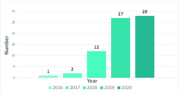
13 Normalization, standardization, and zero-centered, etc. Fig. 4. Number of papers of DL in PA imaging in recent years. For 2020 year’s data, only the quantity before September 15 is calculated.

intervention is also involved for pre-clinical or even clinical

Applications

.

Keywords

learning/network/Net/learned/convolution/GAN/supervise/un

Supervise Is Combined With One Of The Keywords

photoacoustic/optoacoustic to be used for retrieval, then duplicate or unqualified articles (some of them are machine learning) are eliminated. Based on our statistical analysis, the number of papers versus year is shown in Fig. 4. It can be seen that the number on DL used in PA imaging has increased significantly every year. The number classified by category14 is given in Table 1. Next, we will review in detail from the perspective of each task.

A. Pa Image Reconstruction

Image reconstruction is one of the fundamental components for photoacoustic tomography (PAT), which converts raw signals received by ultrasound transducers to the image of initial pressure distribution. It is a challenging task for PA image reconstruction because of the ill-posed nature and the

(Limited-View And Sparse Sampling). In Pat, Image

reconstruction aims to retrieve the initial PA pressure distribution, which indicates the optical absorption of biological tissues. The PA wave propagation at the position r and time t has the pressure p(r,t) given by Eq. (2). The transducer array receives PA signals excited by a short-pulsed laser light at different locations, which are used to form the PA pressure when t=0 by several methods, such as universal

Reconstruction Based On :

14 When counting according to the task category, two papers are about joint task, hence the calculation is repeated twice.

(6)

where Ω0 is the solid angle of the entire detection surface S with respect to a source point at r. The term of square brackets is the back-projection term. These direct reconstructed algorithms can retrieve satisfactory image if the transducers cover enough angle with sufficient element number to detect the PA signals. However, an ill-posed inverse problem is caused by limited-view or sparse view. Meanwhile, the secondary generated artifacts confuse final PA image.

Model-based reconstruction algorithms show flexibility to be applicable in many unfeasible configurations for direct methods. The inverse problem can be formulated by solving

(7)

where p0 is initial PA pressure, y is the received PA data from transducers, A is the PA forward model, R(p0) is regularization term, α decides the properties between data fit and the regularization term. This problem can be solved by traditional optimization, such as iterative soft-thresholding algorithm (ISTA) , GD with repeated iteration. However, these methods are suffering computational complexity and tedious parameters adjustment for different reconstruction tasks. Deep

The

reconstruction of PA images, which are driven by a large number of datasets for training. We will review DL-based PA image reconstruction algorithms of two types.

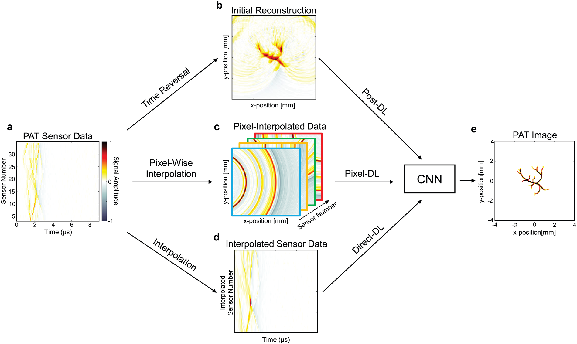
(i) Non-iterative reconstruction. Fig. 5 show three different schemes for non-iterative reconstructions: direct estimation, Fig. 5. Summary of CNN-based deep learning approaches for PAT image reconstruction. Figures adapted with permission from .

PA signals and PA image enhancements via deep learning. Direct reconstruction methods only solve the PA wave equation, which take the PA signals as input and capture the mapping from signal to image.

In , Dominik Waibel established a direct estimation from raw sensor data for PA imaging. 128-element linear detector’s synthetic data were taken into a modified U-net to reconstruct the final initial PA pressure. Similarly, Emran

Mohammad Abu Anas Proposed A Dense Cnn

architecture for beamforming PA data, which consists of five dense blocks with different dilated convolutions. In this paper, the authors investigated the effect of varying speed of sound for proposed method, and verified the robustness on the speed of sound variation. In PAI, the visibility of deeper object can be affected with the optical scattering, which is a non-negligible issue for the precise depth localization applications. To address this issue, Kerrick Johnstonbaugh designed an encoder-decoder network to predict the location of circular target in deep tissue. This work considered both acoustic and optical attenuation into simulation, and it further closed to the reality. Derek Allman used VGG16 to beamform the raw data to detect the point sources, and removed reflection artifact. A real experiment was also demonstrated in this work. Up to now, all of experiments used synthetic simple (point-like) phantoms. In , Johannes Schwab used deep learning to learn the weights in back projection of different channel’s data, and the authors used the Shepp-Logan phantom with random enhancement to verify their method. Furthermore, vessel phantom was first used to train neural network in direct reconstruction. He also proposed

A Data-Driven Regularization Method By Applying

truncated singular value decomposition (SVD) and then

Which

significantly suppressed noise. Hengrong Lan proposed DU-net, which took three different frequencies’ sensor data (2.25MHz, 5MHz and 7.5MHz) as input. In short, DU-net consisted of two U-net, and an additional loss is used to constrain the first U-net. Obviously, the lack of vessel texture structure for raw data, compared with simple phantom, caused a worse result. In , Steven Guan also used vessel phantom to compare different reconstruction schemes, and proposed a new type of input in Fig. 5 (from c to e). Jinchao Feng modified Res-Unet to directly reconstruct the simple phantom, and the results are compared with some varietal U-net models.

Tong Tong used in-vivo data to train the FPnet with a U-net as post-processing. Two types of PA signals (time derivative and normalized original data) are fed into a number of Resblock, and implemented signal-to-image reconstruction

(8)

15 The end of FPnet has a large FC layer, which may cause numerous parameters and overfitting. Some regulations should be applied. In addition, the authors released their code and data in this study. In summary, these direct estimation models capture priori knowledge that being closely related to conventional procedures or not, as shown in Fig. 5 from a to e. On the other hands, PA signal and image enhancement can be performed in the data domain as preprocessing (from a to d in Fig. 5) or in the image domain as postprocessing (from b to e in Fig. 5) instead of solving the PA wave equation. For this scheme, a signal processing or image processing problem usually exists, which is also important for the imaging result of PAM.

By

bandwidth-limited/noise-polluted/spatial-sparse PA signals, even though using a refined reconstruction algorithm. Therefore, PA signal enhancement could obviously improve the PA image quality. Sreedevi Gutta proposed the first neural network to enhance the bandwidth of PA data. A

Channel

bandwidth-limited PA signal as input and predicted full bandwidth signal. Navchetan Awasthi used CNN to de-noise and super resolve (from 50 to 100 detectors) the PA sonogram (sinogram) data in , which solve the sparse and low-SNR problem in signal domain. The experiments contain both simulation and in-vivo experimental cases. Furthermore, they improve the single channel enhanced scheme in and used U-net to de-noise and enhance the bandwidth limited sonogram data . It resolved two issues, and improved the performance compared with previous works. PA signal preprocessing guarantees the quality of reconstruction by compensating the low SNR and distortion of signal induced by limited bandwidth of transducer in data capture procedure.

Spatial-sampling caused issue (limited-view) perhaps should be further explored in image domain. Stephan Antholzer performed sparsely reconstructed image with residual connected U-net. In , the authors also used a U-net to estimate the initial pressure from DAS result

Images. Likewise, Johannes Schwab Used A Cnn To

reconstruct better PA image by feeding 64 detectors and half-view PA image. Light emitting diode (LED) based PA imaging system suffers from low SNR signal due to limited output power. Therefore, the result of LED-based imaging usually has a worse quality. In [73, 74], Emran Mohammad Abu Anas proposed two different architectures, recurrent

Neural Network Based And Cnn (Dense Block) Based

approaches, to enhanced the SNR of input low quality PA image. The blood mimicking phantoms’ data were collected in these works, and generated ground truth by averaging data.

After that, Mithun Kuniyil Ajith Singh used higher laser energy to obtain the ground truth, which are used to train a U-net to enhance the lower SNR image from LED-based

Enhance The Low-Fluence Led-Based Pa Image, Which

replaced the pooling and deconvolution of U-net with discrete wavelet transform and inverse wavelet transform respectively. Ref. also used modified U-net to reconstruct PA image, which divided the model into three parts: feature extraction,

Related Journal Articles & DOI Links

Selected peer-reviewed publications relevant to 12 Lead ECG Acquisition. Click the DOI to access the full paper (may require institutional access).

Why Choose Us?

Bangalore guidance for robotics, Spectre and autonomous systems projects.