Cortical Electrode Interface

Cortical surface registration using unsupervised learning Jieyu Chenga, Adrian V. Dalcaa,b, Bruce Fischla,b,∗, Lilla Z¨olleia,∗, for the Alzheimer’s Disease Neuroimaging Initiative∗∗ aA.A. Martinos Center for Biomedical Imaging, Massachusetts General Hospital, Harvard Medical School,

Usa

bComputer Science and Artificial Intelligence Laboratory, Massachusetts Institute of Technology, USA

Abstract

Non-rigid cortical registration is an important and challenging task due to the geometric complexity of the human cortex and the high degree of inter-subject variability. A con- ventional solution is to use a spherical representation of surface properties and perform registration by aligning cortical folding patterns in that space. This strategy produces accu- rate spatial alignment, but often requires high computational cost. Recently, convolutional neural networks (CNNs) have demonstrated the potential to dramatically speed up volu- metric registration. However, due to distortions introduced by projecting a sphere to a 2D plane, a direct application of recent learning-based methods to surfaces yields poor results.

In this study, we present SphereMorph, a diffeomorphic registration framework for cortical surfaces using deep networks that addresses these issues. SphereMorph uses a UNet-style network associated with a spherical kernel to learn the displacement field and warps the sphere using a modified spatial transformer layer. We propose a resampling weight in com- puting the data fitting loss to account for distortions introduced by polar projection, and demonstrate the performance of our proposed method on two tasks, including cortical par- cellation and group-wise functional area alignment. The experiments show that the proposed SphereMorph is capable of modeling the geometric registration problem in a CNN framework and demonstrate superior registration accuracy and computational efficiency. The source code of SphereMorph will be released to the public upon acceptance of this manuscript at

Keywords:

cortical surface registration, deep learning, unsupervised learning,

∗These Authors Share Senior Authorship

∗∗Data used in preparation of this article were obtained from the Alzheimers Disease Neuroimag- ing Initiative (ADNI) database (adni.loni.usc.edu).

As Such, The Investigators Within The Adni Con-

tributed to the design and implementation of ADNI and/or provided data but did not participate in analysis or writing of this report. A complete listing of ADNI investigators can be found at: http: //adni.loni.usc.edu/wp-content/uploads/how_to_apply/ADNI_Acknowledgement_List.pdf

1. Introduction

Non-rigid shape registration is an important area of research in medical imaging, in particular for establishing cross-subject spatial correspondence in the cerebral cortex. This type of spatial alignment has been shown to improve the statistical power of group functional MRI (fMRI) analysis [1, 2] resulting from the improved correspondence of functional areas.

Due to the geometric complexity of the cortex and the large variability between individuals, cortical surface registration remains a challenging task. Inter-subject surface alignment is commonly driven by geometric features that describe measures of cortical shape (folding), such as sulcal depth or local curvature [3, 4, 5, 6].

A widely used cortical surface registration approach is to map the surface onto the unit sphere in order to perform computations in this canonical domain.

Existing Efforts Are

mainly focused on the adaptation of registration algorithms in the Euclidean space [3, 4, 7]. These aim to optimize a similarity metric between the target and the deformed source vol- umes, regularized by various energies . FreeSurfer registers an individual surface to a probabilistic atlas computed from a representative set of subjects by minimizing the squared difference between the average convexity across subjects and that of the individual, weighted by the inverse variance of the convexity across subjects. The Multimodal Surface Matching tool uses a similarity between the input and reference mesh features in a coarse-to-fine manner. The deformation is driven by aligning local patches around control points, i.e.

vertices of a low resolution mesh, and then propagated to the high resolution input mesh via interpolation. Spherical Demons modifies the classical Demons method using velocity vectors tangent to the sphere. The two-step optimization of classical Demons also holds for the spherical case in which the second step handles the deformation regularization by spherical thin plate spline interpolation. To encourage desirable mathematical properties such as invertibility, diffeomorphic transforms have seen extensive methodological develop- ment, yielding state-of-the-art tools [10, 11]. Unfortunately, since these methods solve an optimization problem for each image pair, they often exhibit long execution times.

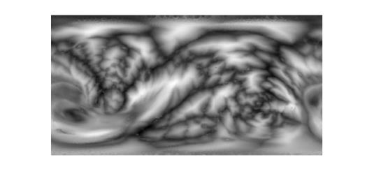
High computational costs have led to an increase in the popularity of supervised [12, 13, 14] and unsupervised [15, 16, 17, 18, 19] learning-based registration algorithms. Consider- ing the difficulty of establishing ground truth spatial correspondences, supervised methods require predictions from existing algorithms , simulations , or both . In contrast, unsupervised methods make use of Spatial Transformer Networks (STN) to warp the moving image in a differentiable way, enabling end-to-end training [15, 17, 21, 22, 23, 18].

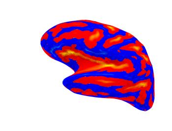
Some unsupervised methods [15, 17, 22] model a stationary velocity field as latent variables representing deformations in a generative probabilistic model. They use a scaling and squar- ing layer for the Lie group exponentiation of the velocity field to generate diffeomorphic transforms, thus guaranteeing topology preservation. These methods have demonstrated high quality performance in registering various types of medical images. Therefore, we build on these concepts when working with surfaces. A more complex model utilizes a vector momentum-parameterized stationary velocity field (vSVF) and jointly optimizes the local regularizer parameterized by a deep network and the registration parameters of the vSVF model for location-varying regularization. In addition to velocity field registration models,

2

sparse learning is also explored for image-template key point matching and a subse- quent interpolation to a dense deformation field via radial basis functions. However, the performance is dependent on the key point selection.

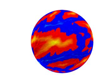
Recent studies have developed geometric convolutional neural networks (CNN) [25, 26, 27, 28, 29, 30] that operate on a spherical manifold to solve classification and detection tasks. To address the distortions introduced by projecting signals to a planar image, regular convo- lutions with increased kernel sizes near polar regions have been utilized . Spherical CNNs encode rotational instead of translational equivariance into the network in Euclidean space to solve classification problems . In SphereNet, the convolution kernel on the sphere has been approximated by encoding the vertex neighborhood information on 2D tangent planes, which enables adapting existing CNN architectures to the omnidirectional setup for object detection and classification tasks . Geometric CNNs (gCNN) also deal with convolution and pooling operations of a CNN on a mesh surface. However, they have so far only been tested on sex classification, using cortical thickness images. A convolutional kernel discretized by an unstructured mesh was recently proposed and evaluated on spheri- cal MNIST classification and 3D object detection tasks . Spherical U-Net proposes a novel Direct Neighbor convolutional kernel based on expansion and contraction process of icosahedron and defines corresponding convolution and pooling operations. Graph con- volutions [31, 32] have been utilized for brain surface data in aligned spectral domains to learn the node-wise prediction , e.g. cortex parcellation and global subject-wise infor- mation , e.g. disease classification or age regression. FastSurfer introduces a full alternative pipeline for FreeSurfer and omits nonlinear surface-atlas registration via fast spherical mapping that quickly maps the volumetric parcellation to cortex using Laplace Eigenfunctions. Most existing work, however, focuses on the construction of spherical con- volutional kernels and, to the best of our knowledge, neural networks have not yet been extended to surface registration. Compared with classification or detection tasks, besides convolution and pooling operations on spheres, a learning-based registration method should address local deformations defined on spheres.

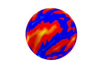
However, Existing Spatial Transformation

networks [34, 35] for spheres only address global deformations, which are not suitable for accommodating nonlinear deformation fields. In this paper, we propose a diffeomorphic framework combining a generative model for surfaces with CNNs to register individual cortical surfaces to an atlas space. This framework adapts conventional VoxelMorph for registering Euclidean images to spherical manifolds.

In order to address the limitations of 2D planar projection, we construct a weighted neigh- borhood graph defined on 2D grids, which accounts for the non-uniform metric tensor of the spherical representation to encode a stationary velocity field. Considering that the 2D projection operation samples the arc-length for each latitude to the same number of points, we also take sampling distortion into account at different latitudes in the likelihood model.

We quantify the performance of our framework through two applications: the generation of cortical parcellations and the alignment of functional activations. The experimental re- sults demonstrate that our framework yields better registration accuracy to state-of-the-art classical methods at a significantly reduced computational cost, and more accurate results compared to current learning-based methods.

Our Contributions Can Be Summarized As:

1. We propose a learning-based framework for spherical surface registration, which pro- vides accurate and efficient performance compared to conventional registration work; 2. We derive an Maximum a Posteriori (MAP) solution for deformation fields in the spherical domain by correcting distortions from planar projection; 3. Different from existing spherical networks, the registration results from our proposed method aid the cortex parcellation as well as various group analyses (i.e. local thick-

Multiple Preset Measures;

4. We explore the use of different features for functional alignment. The remainder of this paper is organized as follows. We first introduce the cortical reg- istration problem, review the conventional VoxelMorph framework, and propose our method and network structure. We then describe two evaluation experiments including cor- tical parcellation and functional alignment, and show results for these experiments. Finally, we present our discussions and conclusions.

2. Methods

Numerous studies using FreeSurfer have demonstrated its efficacy in spherical-based cortical registration. We build on ideas for our surface representation from the FreeSurfer spherical registration and model the unsupervised learning structure for the registration field following VoxelMorph .

2.1. Registration Problem Definition

In the FreeSurfer spherical registration pipeline , surface geometry is encoded as a convexity attribute at each mesh vertex and the representation of the atlas surface is com- puted from a group of adult subjects. In order to register the surfaces of an individual to the atlas space, first a white matter mesh is generated and mapped to the unit sphere by minimizing metric distortion . Next, an optimal rotational alignment is computed by global search over two rotation angles on the sphere. Then a 2D canonical warp is computed to align the subject’s convexity pattern with that of the mean pattern encoded in the atlas, by minimizing the mean squared difference, weighted by the inverse of the atlas variance.

Our goal is to compute this canonical warp using a CNN framework. Let Sx be the unit sphere and Ix the corresponding scalar field over the sphere (e.g. sulcal depth or curvature) projected into 2D longitude/latitude parameterization. Let Ia be the atlas mean image as defined in FreeSurfer, and M and N be the number of image rows and

2...Σ2

MN) be a diagonal matrix where each diagonal element denotes the variability of the corresponding feature at a particular vertex as defined in the FreeSurfer atlas variance image. The goal is to find the spatial transformation Φ : S2 →S2 given Ix and Ia that maximizes the a posteriori probability of the transform assuming certain smoothness priors on the warp.

2.2. Voxelmorph

We assume a diffeomorphic deformation based on a stationary velocity field v, denoted as Φv, and adapt a generative probabilistic model following VoxelMorph . VoxelMorph uses Maximum a Posteriori (MAP) estimation to obtain the most likely velocity field v∗at each voxel/pixel given a pair of images. VoxelMorph models the prior probability of v as a zero-mean multivariate normal distribution, p(v) = N(v; 0, Σv), where Σv is the covariance matrix. An individual image can be estimated by warping the FreeSurfer atlas, thus we model the warped image Ix ◦Φv as p(Ix|v; Ia) = N(Ix ◦Φv; Ia, Σa), where Φv is the inverse transformation of the atlas warping to the individual. The aim is to maximize the posterior

R

v p(v,Ix;Ia)dv, where the marginalization over v is intractable. In this case, a variational approximation qψ(v|Ix; Ia) is adopted with parameters ψ, by minimiz- ing its dissimilarity, Kullback–Leibler (KL) divergence, with the true posterior probability.

For simplicity, the approximate posterior qψ(v|Ix; Ia) is restricted to a multivariate normal distribution N(µv|Ix;Ia, Σv|Ix;Ia) where µv|Ix;Ia and a diagonal Σv|Ix;Ia are functions estimated with a U-Net core , as shown in Fig. 2.

Using the above assumptions, maximizing the posterior probability can be approximated

By Minimizing The Following Loss:

L(ψ; Ix, Ia) = −Eq[log p(Ix|v; Ia)] + KL[qψ(v|Ix; Ia)||p(v)],

(1)

where Eq[·] operates the expectation computation given the distribution q and q is short for qψ(v|Ix; Ia). The first term describes the reconstruction loss and the second term is a KL divergence term, encouraging the estimated posterior probability qψ(v|Ix; Ia) to be close to the prior p(v). VoxelMorph encourages the smoothness of the velocity field v by setting

V

= Λv = λL, where the parameter λ controls the scale of the velocity field and L is the graph Laplacian matrix defined on the Euclidean grid. L is computed as L = (D −A), where A is the neighborhood adjacency matrix and D is the graph degree matrix. Thus,

Eq. (1) Can Be Rewritten As:

L(ψ; Ix, Ia) = −Eq[log p(Ix|v; Ia)] + KL[qψ(v|Ix; Ia)||p(v)]

(2)

where K is the number of samples vk ∼q used to approximate the expectation. We use K = 1. We treat the fixed atlas Ia and the warped individual image Ix ◦Φv as MN × 1 vectors. We denote this naive application of the registration of 2D projected images as the 2D VoxelMorph method and it serves as a benchmark in our experiments.

Θ=0

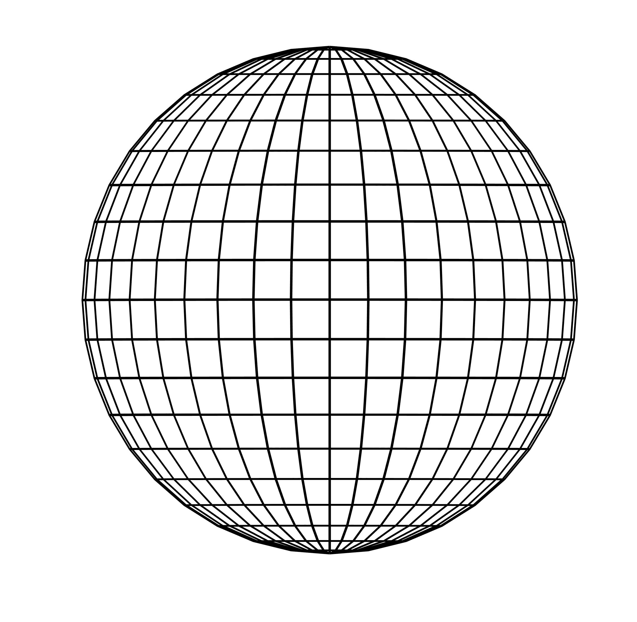
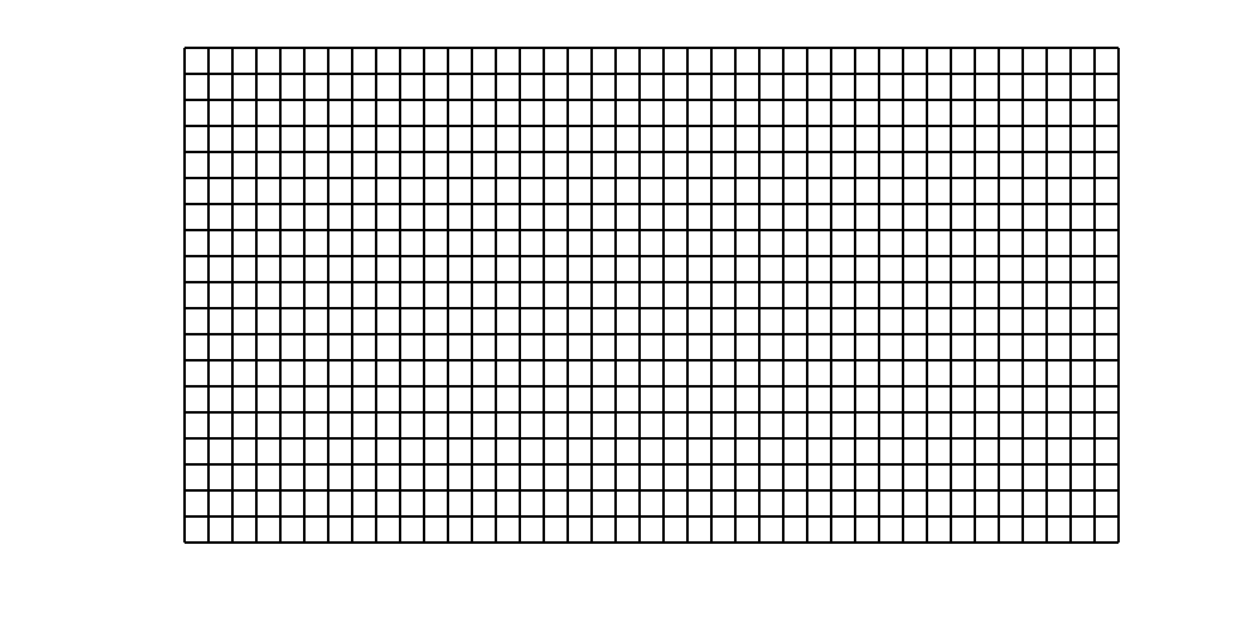
Figure 1: Illustration of a spherical mesh and its corresponding 2D rectangular grids by planar projection. ϕ and θ denote the longitude and latitude respectively. Regions with higher latitude, e.g. red dots here, have denser samplings compared to regions with lower latitude (e.g. blue dots), yielding greater distortions.

The regions crossing θ = 0 (green line) become non-adjacent due to the cutting and flattening operations. Unfortunately, the 2D projection step introduces two main problems, as shown in Fig. 1: • varying level of distortions with different latitudes (distortion increases from the equa-

Tor To The Poles); And

• inability to represent the periodic property of θ and the geometry of the poles (an enclosed spherical surface is projected onto a rectangular image region, introducing discontinuities at the image borders).

Hence, the 2D VoxelMorph method over-weights the alignment for near-pole regions, yielding misalignment in most regions even compared to global rigid registration as shown in Section 3.

2.3. Proposed Method: Spheremorph

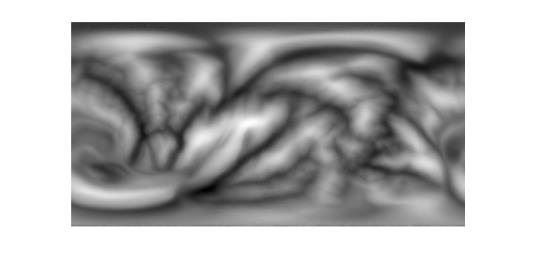
To address the above issues, we propose SphereMorph. We start by defining the registra- tion problem in the spherical domain. The spherical representation of an individual’s surface is first rotated for a rigid alignment with the atlas, as in FreeSurfer. The spherical surface is parameterized by the longitude θ and latitude ϕ and sampled to an M ×N two-dimensional image with a geometric or functional feature, e.g. convexity, assigned as a pixel intensity measure.

Prior correction. We assume that the displacement field is smooth on the sphere consid- ering the anatomical continuity via a graph Laplacian regularizer. We define a neighbour connectivity graph GS on the spherical manifold and represent the velocity with respect to Cartesian coordinates as a signal defined on this graph. Let T denote the conversion from polar to Cartesian coordinates, that is [x, y, z]T = T ([θ, ϕ]) = [sin ϕ cos θ, sin ϕ sin θ, cos ϕ]T,

6

..

Sampling

Figure 2: The proposed cortical surface registration workflow (SphereMorph). The input spherical rep- resentation is first rigidly aligned to the atlas using convexity patterns and then projected onto a polar coordinate system. The Spherical U-Net core takes parameterized input image Ix and atlas mean image Ia as inputs and estimates the distribution, µv|Ia;Ix and Σv|Ia;Ix, of the velocity field v, which is then sampled and integrated using scaling and squaring steps to generate the deformation field Φv.

then the geodesic velocity at each vertex V eri(θi, ϕi), i ∈[1, 2, .., MN] is given by v′ = f(v) = [vx(θi, ϕi), vy(θi, ϕi), vz(θi, ϕi)]T = T (Φv([θi, ϕi])) −T ([θi, ϕi]). Each vertex on the projected image is considered as a node and each grid edge connecting two adjacent nodes as their edge in GS. We connect leftmost and rightmost nodes due to the periodicity in longitude. The weight of the connection between vertices in GS varies with location to account for the horizontal edge distance on the spherical surface which is proportional to sin ϕ. Thus, we define the weight of each grid edge connecting vertices

If

ϕi̸ = ϕj, θi = θj.

(3)

We construct the corresponding neighborhood adjacency matrix AS with entries ASij = wij and the degree matrix DS with diagonal entries DSii = P

J Wij. Finally, We Denote The

Laplacian of this weighted graph as LS = DS −AS and define the covariance of geodesic

Velocity As Σ−1

v′ = ΛSv = λLS. Intuitively, this formulation can be seen as increasing the regularization near the poles, where the Euclidean distance between mesh nodes is small, and decreasing the weighting near the equator where the Euclidean distances are larger.

Distortion correction. For VoxelMorph, which deals with Euclidean image registration, the sampling of grid points is equally distributed. However, a spherical parameterization

7

leads to denser sampling grids for regions at higher latitudes as shown in Fig. 1. Thus, we assign mesh locations from these regions lower weights in computing the data-fitting term, by introducing a diagonal matrix S ∈RMN×MN with each diagonal entry encoding the resampling weight Sii = sin ϕi for each vertex V eri(θi, ϕi) and model p(Ix|v; Ia) = N(Ix ◦Φv; Ia, S−1Σa). The first data-fitting term in Eq. (1) is then modified as:

(Ia −Ix ◦Φvk)Tς−1

a S(Ia −Ix ◦Φvk).

(4)

Loss function. Starting with Eq. (1) and taking into account the spherical geometry, we

Arrive At The Below Objective Function:

L(ψ; Ix, Ia) = −Eq[log p(Ix|v; Ia)] + KL[qψ(v|Ix; Ia)||p(v)]

I

+ const.

(5)

where µv′|Ix;Ia = f(µv|Ix;Ia) and Σv′|Ix;Ia = f(Σv|Ix;Ia). The first term in Eq. (5) is the data- fitting term, which encourages matching surfaces after warping and the second term drives the posterior to approximate the smoothness prior defined on a spherical grid.

Network structure. Figure 2 illustrates the individual stages task fmriof our pipeline. For a given vertex at location (θ, φ), we utilize inverse gnomonic projection, which maps points on the tangent plane to the spherical surface as in SphereNet , to obtain the corresponding locations on the projected image for the neighbor vertex on its tangent plane.

We implement the convolution and pooling operations in each 3 × 3 local tangent patch shown in Figure 1 and build a UNet core , which contains four downsampling and four upsampling layers. Following the sampling layer, seven scaling and squaring operators take the layer output, or velocity field, and return a diffeomorphism Φ. 2D VoxelMorph uses a dense spatial transformer layer on (θ′, φ′) after displacement to retrieve the warped image while SphereMorph warps the image by computing the interpolation grids as ((θ′ +2π) mod 2π, φ′) for transformer layer. The model is implemented in Keras with a Tensorflow backend and the ADAM optimizer as part of the VoxelMorph package. We set the hyperparameter λ = 3 × 107, the learning rate to 1 × 10−5, and trained our dense model for 200 epochs, by which point the loss had converged as shown in Figure 3. All experiments were conducted for all CNN-based methods. The source code of SphereMorph will be released to the public upon acceptance of this manuscript at https://github.com/voxelmorph/spheremorph.

3. Experimental Setup

To demonstrate the accuracy and efficiency of the proposed registration framework, SphereMorph, we used two sets of experiments, cortical parcellation and fMRI group anal- ysis, on two independent test data sets.

Loss

Figure 3: Line plot of the converging loss function over training epochs.

3.1.1. Training Data Set:

The spherical atlas from FreeSurfer served as the fixed image in our model. As train- ing data, we used the surface convexity maps of the left hemispheres of 800 randomly selected subjects from the ADNI1 cohort that was released as part of the publicly available Alzheimer’s Disease Neuroimaging Initiative (ADNI) (http://adni.loni.usc.edu/) and was processed by FreeSurfer v5.1.

The Adni Was Launched In 2003 As A Public-

private partnership, led by Principal Investigator Michael W. Weiner, MD. The primary goal of ADNI has been to test whether serial magnetic resonance imaging (MRI), positron emission tomography (PET), other biological markers, and clinical and neuropsychologi- cal assessment can be combined to measure the progression of mild cognitive impairment (MCI) and early Alzheimers disease (AD). The ADNI dataset consists of longitudinal T1- weighted scans from 836 subjects that are divided into four classes: elderly controls (n = 252), early mild cognitive impairment (eMCI, n =215), late MCI (lMCI, n = 176), and AD (n = 193). The subjects were scanned on average 4.8 times (minimum: a single time; maximum: 11 times; 4013 scans in total), with a mean interval between scans equal to 286 days (minimum: 23 days, maximum: 1567 days). The mean age at baseline of the subjects was 75.1 ± 6.6 years. Since the ADNI project spans multiple sites, different scan- ners were used to acquire the images; further details on the acquisitions can be found at http://adni.loni.usc.edu/data-samples/adni-data-inventory/.

3.1.2. Test Data Sets:

(1) We used FreeSurfer-processed MRI scans of 39 subjects from a cohort recruited by scans were acquired on a 1.5T Vision system (Siemens, Erlangen Germany). T1-weighted magnetization-prepared rapid gradient echo (MP-RAGE) scans were obtained according to the following protocol: two sagittal acquisitions, FOV = 224, Matrix = 256×256, Resolution

9

= 1 × 1 × 1.25mm3, TR = 9.7 ms, TE = 4 ms, Flip angle = 10, TI = 20 ms, TD = 200 ms. Two acquisitions were averaged together to increase the contrast-to-noise ratio. For the cortical parcellation experiment, we separated the data set into two: 9 validation subjects and 30 held-out test subjects. All subjects have 34 cortical areas manually annotated , making them ideal for evaluating registration accuracy.

(2) Additionally, we used another set of 100 unrelated young and healthy subjects from the Human Connectome Project (HCP) as a second test set. The HCP project used state-of-the-art fMRI hardware and acquisition parameters in a sample of highly educated, healthy subjects. For each subject, seven task fMRI sessions were collected, including work- ing memory, gambling, motor, language, social cognition, relational processing and emotional processing, totaling 48:30 min of fMRI data. The acquisition parameters and minimal pre- processing of these data have been described extensively elsewhere [41, 42].

3.2. Baselines

We compared our proposed registration method to rigid registration on the sphere (i.e. two rotations) and four other nonlinear registration methods: a 2D version of VoxelMorph, Multimodal Surface Matching (MSM) , Spherical Demons (SD) , and FreeSurfer (FS) spherical registration . We chose the sulcal depth as the input feature for all registration methods. Additionally, we also explored the usage of the curvature and T1/T2 maps together with sulcal depth in the HCP functional group analysis experiments. Additionally, we also explored the usage of the curvature and T1/T2 maps together with sulcal depth in the HCP functional group analysis experiments. We trained 2D VoxelMorph using the same training set as described above and selected the hyperparameter λ that yielded the best performance on the validation set. MSM is a surface-based registration approach that offers significant flexibility with regards to the set of features that are used to drive the spatial alignment. MSM drives the deformation via aligning local patches around control points in a multi-resolution fashion. It is implemented on CPU using a fast, multi-resolution, discrete optimisation scheme, offering significant computational speed-up compared to other classical methods. We ran MSM over three resolution levels with five iterations per level. Specifically, we set the regularization parameters as (0.1, 0.2, 0.3) for the parcellation experiments. For the functional group analysis experiments, we relied on the publicly released MSMSulc results which were generated by running MSM with high regularization parameters (10, 7.5, 7.5) and using the sulcal depth feature. Compared to the low regularization, MSM with high regularization has been demonstrated to yield lower group alignment in folding patterns but smaller area distortions , which leads to better functional alignment after following registration steps using myelin maps. Spherical Demons, a fast diffeomorphic landmark-free surface registration tool implements the regularization for its objective function via iterative Gaussian smoothing. We explored a range of smoothing iteration numbers (5, 10, 15, 20) to optimize performance and used the results of 10 iterations.

3.3. Evaluation

To evaluate registration accuracy, we relied on the resulting spatial transformations to project the atlas parcellation back to individual scan space. For an accurate registration

10

solution, the test subjects cortical parcellations will resemble the manually outlined versions. In order to quantify how well they match, we computed the Dice overlap coefficient , the overall Mean Minimum Distance (MMD) as well as the individual MMD measures for each anatomical region. The Dice overlap coefficient, Dice(M, A) = 2 ·

Rm+Ra, Quantifies

the surface area overlap (RM∩A) between manual (RM) and automatic method-generated parcels (RA) and the MMD describes the discrepancy between the parcellation boundaries: MMD(M, A) = 1/N · Σid(mi, ai) where d(mi, ai) denotes the Euclidean distance between a vertex mi on a manual boundary and its corresponding closest vertex ai on an automatic method-generated boundary. Additionally, we also tested how consistently the various regis- tration methods aligned anatomical features, such as convexity/sulcal depth and curvature.

In the second set of experiments, we mapped all individuals within the group to the HCP’s 2mm standard grayordinates space , using the displacement field, then computed group maps of task-evoked activations. To evaluate the quality of the group alignment quan- titatively, we computed average correlations between the group-average and the projected individual activation maps across 86 task contrasts derived from the seven fMRI tasks.

4.1. Computational Efficiency

Table 1 summarizes registration accuracy and computation time for all methods. All the compared methods take spherical cortical surfaces as input, which are generated by brain surface tessellation including fixing topological defects and inflation to the sphere from volumetric segmentation. For a brain surface with 120k-150k vertices, it takes around 0.9h and 0.25h CPU computation time for surface tessellation and inflation, respectively. The comparison of registration time illustrates that the proposed method ran approximately 20 times faster than the conventional registration method in FreeSurfer. On a CPU, the default FreeSurfer pipeline takes around 13 minutes to complete the spherical registration. The total computation time of our proposed framework is approximately 0.74 minutes, including the initial alignment, deep network deployment, and displacement field mapping. With GPU acceleration, the computation time of our method can be reduced to 0.65 minutes, where the deep network deployment is accomplished within a second. Compared with other registration methods including MSM and Spherical Demons (SD), CNN-based methods provide more than an order of magnitude improvement in execution speed.

4.2.1. Parcellation Accuracy

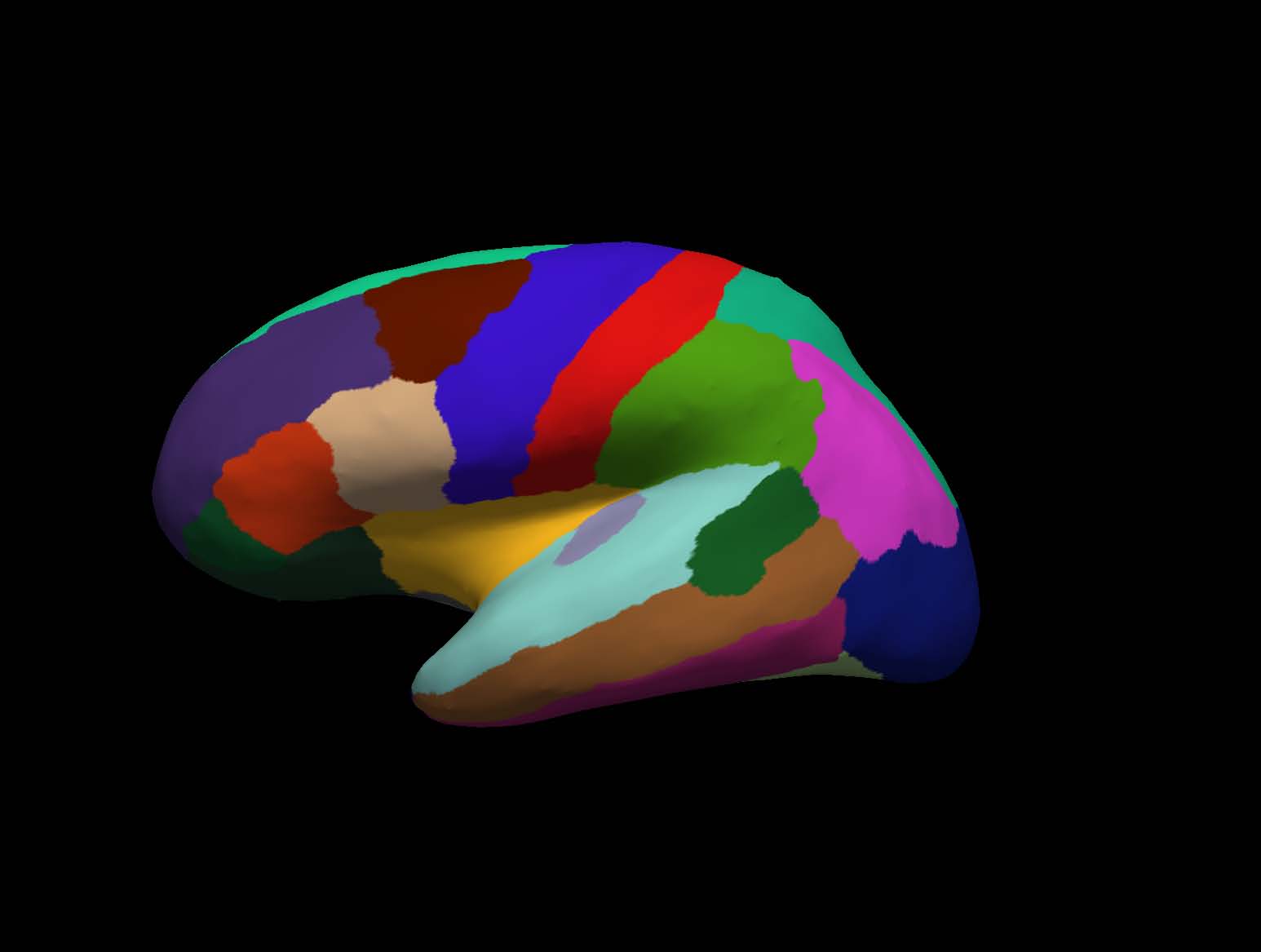
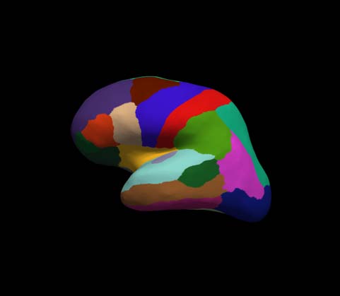
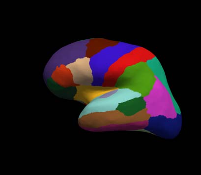
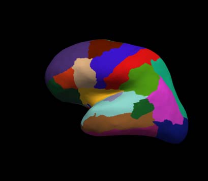
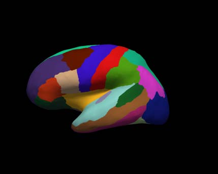
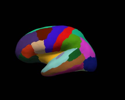
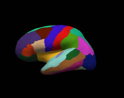
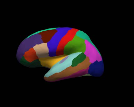
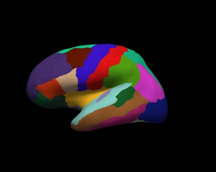
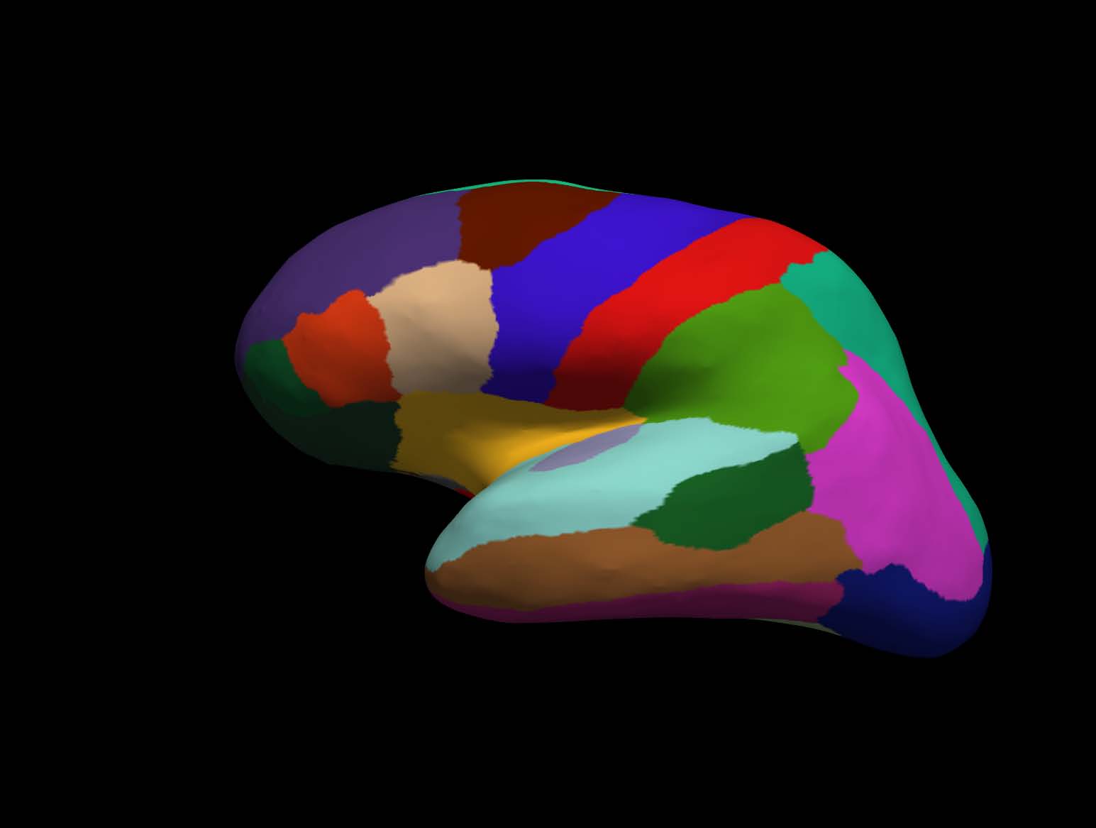
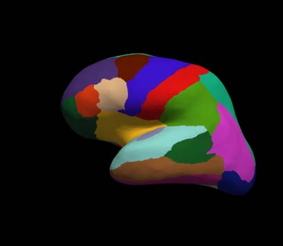
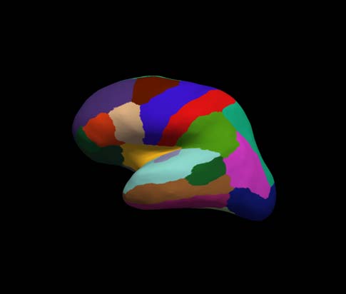
Figure 4 shows representative cortical segmentation results from all the methods on two randomly selected test subjects from the ADRC dataset. The 2D VoxelMorph-estimated annotation exhibits large differences compared to the ground truth in the lateral occipital regions (marked by white arrows), while FreeSurfer and SphereMorph provide results close to the manual annotations. Figure 5 displays the two subjects for which our proposed method yields the lowest and highest overall Dice values.

Subject 2

Figure 4: Cortical parcellation results for two example subjects from the ADRC dataset. For each subject, the upper rows show the cortical parcellation estimated by different registration methods and the lower rows give a closer view of the parcellation comparison in the lateral occipital region (white arrows) with manual parcellation boundary superimposed.

Table 1: Overview of registration accuracy and CPU run time for rigid alignment, 2D VoxelMorph, MSM, Spherical Demons, FreeSurfer spherical registration, and our proposed SphereMorph. SphereMorph performs in a comparable manner with FreeSurfer, while being roughly 20 times faster.

Related Journal Articles & DOI Links

Selected peer-reviewed publications relevant to 12 Lead ECG Acquisition. Click the DOI to access the full paper (may require institutional access).

Why Choose Us?

Bangalore guidance for robotics, Spectre and autonomous systems projects.