Dialysis Machine Monitoring

Monitoring and explainability of models in production Janis Klaise * 1 Arnaud Van Looveren * 1 Clive Cox 1 Giovanni Vacanti 1 Alexandru Coca 1

The Deployment Stage. Monitoring Deployed Mod-

els is crucial for continued provision of high qual-

Include Model Performance And Data Monitoring,

detecting outliers and data drift using statistical techniques, and providing explanations of historic predictions. We discuss the challenges to success-

Areas With Some Recent Examples Of Production

ready solutions using open source tools.

1. Introduction

In recent years, the problem of how to deploy and scale machine learning models has been made easier by open source tools such as Seldon Core (Cox et al., 2018), KF- Serving (KFServing, 2019), Kubeflow (Kubeflow, 2018) and MLFlow (Zaharia et al., 2018). One of the big chal- lenges in MLOps is to design systems that monitor live deployments and take action or raise alerts when events im- pacting model performance are encountered (Diethe et al., 2019). Traditional application monitoring involves logging such core metrics as request latency, frequency and server load with the intention of ensuring uninterrupted, high qual- ity service. On the other hand, it is more demanding to maintain the same level of service for machine learning applications. We identify four additional areas following model deployment which are key for the success of the

4. Explaining Model Predictions

*Equal contribution 1Seldon Technologies Ltd, London, United Workshop on Challenges in Deploying and Monitoring Machine

Learning Systems (Icml 2020)

Firstly, it is critical to ensure model performance does not degrade in a production setting. Inability to detect model performance degradation can lead to stale models and in- creased technical debt (Breck et al., 2017; Sculley et al., 2015). Whilst trained models usually come with perfor- mance metrics on offline test sets, this does not guarantee similar performance in live systems.

Figure: System Model & Simulation Flow for Dialysis Machine Monitoring

Secondly, measuring model performance implies having timely access to labels for live data which are seldom avail- able due to operational and financial constraints. In the absence of labels it is critical to monitor the statistics of input data and output predictions as these can serve as a proxy for model performance (Breck et al., 2017).

Thirdly, to be truly useful the monitoring system requires functionality to determine when significant changes to data and predictive distributions happen, also known as drift detection. A related task is to identify incoming data points which fall outside the training data distribution, also known as outlier detection. These questions are statistical in nature and often require separate models which makes it more difficult to provide general solutions.

Finally, it is important to build trust in machine learning systems and make the decision process transparent. Many models are often “black boxes” whose internal processing is not well understood even by trained data scientists. The field of explainable AI provides numerous approaches to the problem of explaining model predictions, some of which are uniquely suited for deployed models.

In the following sections we discuss the key challenges in these areas from an algorithmic as well as infrastructure perspective and point to existing solutions using open source technologies.

2.1. Performance And Metrics

Ensuring high model performance in live deployments is arguably the most important aspect of monitoring machine learning systems. However, performance metrics used to develop the models depend on the availability of labels. For live data the number and frequency of collected labels de- pends on the application. For example, in high-frequency

Arxiv:2007.06299V1 [Stat.Ml] 13 Jul 2020

Monitoring and explainability of models in production time-series prediction or internet ad serving labels are auto- matic and near real-time whilst for many other applications labels are expensive to produce, potentially unreliable and with long time delays following a prediction. For instance, consider a medical diagnostic system based on image recog- nition. Labelling even small samples of the data presented to such a system can be challenging since it is time con- suming and requires domain knowledge. Label noise can also occur due to disagreements between annotators (Louie et al., 2010; Khoo et al., 2012; Bridge et al., 2016). It is however still crucial to report metrics which inform whether the performance of the deployed model is satisfactory.

In the perfect scenario of full and immediate label avail- ability the calculation of performance metrics is straightfor- ward, however some challenges remain on the infrastructure and decision making level. Firstly, the labels have to be fed into some system that then calculates metrics on the fly. This can be a separate system or as part of the model deployment. For example, Seldon Core provides a dedi- cated /send-feedback API endpoint accepting labels and performing user-defined metric calculations which can be standard ML metrics (e.g. accuracy for classification models) or custom, business-specific metrics (e.g. key KPIs derived from performance metrics). Secondly, metrics are inherently stateful—updating a metric with new values in- volves using the metric value from the previous step. This is in contrast with deployed models which are static over the lifetime of the model. Whilst recent open source libraries provide solutions to such online learning of metrics and histograms (Bolmier et al., 2019), the engineering effort of ensuring a metrics component does not lose its state and does not go out of sync (e.g. if the metrics component is scaled up to multiple instances) remains. Thirdly, one must decide on appropriate time periods for calculating metrics.

For some use cases metrics over the lifetime of the deploy- ment are most useful while for others static or dynamic time windows based on real time or request frequency are more appropriate. Finally, even with accurate knowledge of label- dependent metrics one must set some threshold or decision rule for when to raise alerts when metrics deteriorate. Such thresholds require domain knowledge and can be difficult to set appropriately to limit the number of false alarms. Al- ternatives based on change-point detection may prove to be more robust (Bifet, 2017).

In the more common scenario of scarce labels it is com- mon to use label-independent metrics as a proxy for model performance (Breck et al., 2017). This includes designing metrics for monitoring live input data and model predictions.

In contrast to performance metrics, appropriate metrics de- pend on the data type. Image, text and tabular data will have different metrics of interest. Even in the widespread case of tabular data, metrics will be different based on the type of features. For example, whilst we can monitor the feature-wise moments and order statistics of numerical fea- tures, frequency based measures are more appropriate for categorical features. Going beyond pointwise metrics, fast algorithms for approximate online histograms (Ben-Haim & Tom-Tov, 2010) can provide much richer insight into the live data distributions. Nevertheless, a fundamental drawback of univariate metrics is that correlations between features are not captured. Multivariate metrics such as covariance matrices and multivariate histograms remain difficult to im- plement due to the increased computational cost and curse of dimensionality as well as the need for an online update rule. We discuss multivariate approaches in the context of detecting drift in Section 2.3.

2.2. Outlier Detection

Machine learning models often fail to generalize outside of the training data distribution (Recht et al., 2019; En- gstrom et al., 2019; Hendrycks & Dietterich, 2019). Further- more, models are typically not well calibrated (Guo et al., 2017) which can lead to overconfident predictions on out- of-distribution instances (Lakshminarayanan et al., 2017).

Outlier detection is therefore key to flag anomalies whose model predictions we cannot trust and should not use in a production setting. The type of outlier detector for a specific application depends on the modality and dimensionality of the data, availability of labeled normal and outlier data, and whether the detector is pre-trained (offline) or updated on- line. The pre-trained detector can be deployed as a separate static machine learning model while the online detector is deployed as a stateful application. Labeled outlier data is often scarce, making the problem semi-supervised at best.

Open source libraries such as Alibi Detect (Van Looveren et al., 2020) and PyOD (Zhao et al., 2019) provide a wide range of mainly unsupervised off-the-shelf outlier detectors which can be tailored to the specific problem setting.

It is important to note that the problem of unsupervised anomaly detection for real-world data (e.g. natural images or noisy time series) is far from solved. At the heart the problem is one of reliable density estimation. The quality of the estimator however depends on the modality and the data set. Different studies on image data (Nalisnick et al., 2019; Choi et al., 2018) also illustrate that generative density mod- els can assign higher likelihood values to out-of-distribution instances compared to inlier data. Contrary to most machine learning tasks, the unsupervised training objective is only a proxy for the actual performance of the detector.

2.3. Drift Detection

While outliers refer to individual instances, data drift or shift detection checks whether two samples are drawn from the same underlying distribution or not via a statistical hypothe- sis test. The goal of the drift detector is therefore to identify Monitoring and explainability of models in production when the distribution of the requests for the deployed model starts to diverge from the training data and model predictions become unreliable. We can further distinguish covariate shift from label shift of the model predictions. In the case of covariate shift the input data distribution p(x) changes while the conditional label distribution p(y|x) remains unchanged.

Label shift happens when p(y) changes but the conditional p(x|y) does not. In order to make drift detection work in practice on high- dimensional data such as images, the incoming data first undergoes a dimensionality reduction step before applying the hypothesis test. Rabanser et al. (2019) observe that ran- domly initialized encoders and black box dimensionality reduction introduced by Lipton et al. (2018) are promising pre-processing methods. This is followed by a two-sample test such as the maximum mean discrepancy (Gretton et al., 2012) for the multivariate case in combination with a permu- tation test to obtain p-values. Alternatively, a feature-wise Kolmogorov-Smirnov test (Smirnov, 1939) is run with Bon- ferroni or False Discovery Rate (Benjamini & Hochberg, 1995) p-value correction for multivariate data.

Drift detection informs the user when the model should be retrained which is especially important in applications where model performance feedback is not readily available.

Malicious data drift, which significantly harms model per- formance, is of special importance. Vacanti & Van Looveren (2020) show that drift detection on an instance level adver- sarial score is effective at identifying underlying malicious data shift. Alibi Detect (Van Looveren et al., 2020) provides all the aforementioned drift detection functionality under a common API.

2.4. Deploying Model Monitoring

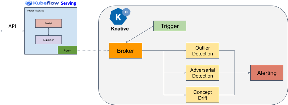
The techniques discussed above need to be deployed along- side the running models but in a manner which does not adversely affect their core performance. Recent inference deployment projects such as KFServing and Seldon Core which run on the Kubernetes container orchestration plat- form solve this by utilizing the eventing based project KNa- tive (KNative, 2019) which allows serverless components to be connected to event streams. The serverless KNative project makes it possible to scale services down to zero if no requests are being received and scale up as demand increases. This allows monitoring components to scale as needed. Figure 1 shows the resulting architecture.

Incoming low latency requests run as normal with a payload logging solution sending events containing model request and response payloads to a KNative broker which can farm these out as desired via programmable triggers to serverless components such as outlier, drift and adversarial detection modules. Further eventing components can be added to feed off events produced by these components to send onwards to, Figure 1. Asynchronous ML monitoring implementation with KF- Serving and KNative eventing.

for example, alerting or storage modules. The architecture provides a clean separation of concerns between the model and its later analysis components each of which can be scaled separately.

3.1. The Need For Model Explanations

Instance level machine learning model explanations are de- sirable for multiple reasons. They allow the user to build trust in the predictions made by the deployed machine learn- ing system and improve transparency. The user can verify which factors contributed to certain predictions, introduc- ing a layer of accountability. Model introspection is also increasingly important with the rise of pre-trained models (e.g. Kolesnikov et al. (2019) for computer vision or Wolf et al. (2019) for language tasks) which are only fine-tuned for a specific downstream task. The data used during the pre-training stage is not curated by the user of the down- stream task and can create harmful model biases, poten- tially leading to unfair outcomes. Buolamwini & Gebru (2018) highlight the importance of representative and unbi- ased training sets in computer vision to avoid discrimination while Bolukbasi et al. (2016) reveal that even the pre-trained word embeddings Word2Vec contain societal gender bias.

Model introspection goes hand in hand with other monitor- ing practices such as anomaly or drift detection. When an instance is flagged as an outlier, explanation methods can help determine whether the model prediction on the instance can be trusted and acted on.

The suitability of an explanation method depends on the data modality, type of model (e.g. tree-based or neural net- work) and prediction task (e.g. classification or regression).

Most commonly used explanation methods also need heuris- tics and make assumptions about key components of the explanation generating process such as the background val- ues for each feature (e.g. SHAP (Lundberg & Lee, 2017), Integrated Gradients (Sundararajan et al., 2017), Anchors (Ribeiro et al., 2018), Contrastive Explanations (Dhurandhar et al., 2018)), local model behaviour (e.g. local linearity for

Related Journal Articles & DOI Links

Selected peer-reviewed publications relevant to 12 Lead ECG Acquisition. Click the DOI to access the full paper (may require institutional access).

Why Choose Us?

Bangalore guidance for robotics, Spectre and autonomous systems projects.